Abstract. I introduce a Markov chain Monte Carlo (MCMC) scheme in which sampling from a distribution with density $\pi(x)$ is done using updates operating on an “ensemble” of states. The current state $x$ is first stochastically mapped to an ensemble, $(x^{(1)},\ldots,x^{(K)})$. This ensemble is then updated using MCMC updates that leave invariant a suitable ensemble density, $\rho(x^{(1)},\ldots,x^{(K)})$, defined in terms of $\pi(x^{(i)})$ for $i\,=\,1,\ldots,K$. Finally a single state is stochastically selected from the ensemble after these updates. Such ensemble MCMC updates can be useful when characteristics of $\pi$ and the ensemble permit $\pi(x^{(i)})$ for all $i\in\{1,\ldots,K\}$, to be computed in less than $K$ times the amount of computation time needed to compute $\pi(x)$ for a single $x$. One common situation of this type is when changes to some “fast” variables allow for quick re-computation of the density, whereas changes to other “slow” variables do not. Gaussian process regression models are an example of this sort of problem, with an overall scaling factor for covariances and the noise variance being fast variables. I show that ensemble MCMC for Gaussian process regression models can indeed substantially improve sampling performance. Finally, I discuss other possible applications of ensemble MCMC, and its relationship to the “multiple-try Metropolis” method of Liu, Liang, and Wong and the “multiset sampler” of Leman, Chen, and Lavine.

Introduction

In this paper, I introduce a class of Markov chain Monte Carlo methods that utilize a state space that is the $K$-fold Cartesian product of the space of interest — ie, although our interest is in sampling for $x$ in the space ${\cal X}$, we use MCMC updates that operate on $(x^{(1)},\ldots,x^{(K)})$ in the space ${\cal Y}\,=\,{\cal X}^{K}$.

Several such methods have previously been proposed — for example, Adaptive Directive Sampling (Gilks, Roberts, and George, 1994) and Parallel Tempering (Geyer, 1991; Earl and Deem, 2005). The “ensemble MCMC” methods I introduce here differ from these methods in two fundamental respects. First, use of the space ${\cal Y}\,=\,{\cal X}^{K}$ is temporary — after some number of updates on ${\cal Y}$, one can switch back to the space ${\cal X}$, perform updates on that space, then switch back to ${\cal Y}$, etc. (Of course, one might choose to always remain in the ${\cal Y}$ space, but the option of switching back and forth exists.) Secondly, the invariant density for an ensemble state $(x^{(1)},\ldots,x^{(K)})$ in the ${\cal Y}$ space is proportional to the sum of the probabilities of the individual $x^{(k)}$ (or more generally a weighted sum), whereas in the previous methods mentioned above, the density is a product of densities for each $x^{(k)}$. As a consequence, the properties of the ensemble methods described here are quite different from those of the methods mentioned above.

I expect that use of an ensemble MCMC method will be advantageous only when, for the particular distributions being sampled from, and the particular ensembles chosen, a computational short-cut exists that allows computation of the density for all of $x^{(1)},\ldots,x^{(K)}$ with less than $K$ times the effort needed to compute the density for a single state in ${\cal X}$. Without this computational advantage, it is hard to see how performing updates on ${\cal X}^{K}$ could be beneficial.

In this paper, I mostly discuss one particular context where such a computational short-cut exists — when the distribution being sampled has the characteristic that after changes to only a subset of “fast” variables it is possible to re-compute the density in much less time than is needed when other “slow” variables change. By using ensembles of states in which the slow variables have the same values in all ensemble members, the ensemble density can be quickly computed. In the limit as the size of the ensemble grows, it is possible using such a method to approach the ideal of updating the slow variables based on their marginal distribution, integrating over the fast variables.

I apply these fast-slow ensemble MCMC methods to Gaussian process regression models (Rasmussen and Williams 2006; Neal 1999) that have a covariance function with unknown parameters, which in a fully Bayesian treatment need to be sampled using MCMC. The computations for such models require operations on the covariance matrix whose time grows in proportion to $n^{3}$, where $n$ is the number of observations. If these computations are done using the Cholesky decomposition of the covariance matrix, a change to only the overall scale of the covariance function does not require recomputation of the Cholesky decomposition; hence this scale factor can be a fast variable. If computations are done by finding the eigenvectors and eigenvalues of the covariance function, both an overall scale factor and the noise variance can be fast variables. I show that ensemble MCMC with either of these approaches can improve over MCMC on the original state space.

I conclude by discussing other possible applications of ensemble MCMC, and its relationship to the “multiple-try Metropolis” method of Liu, Liang, and Wong (2000), and to the “multiset sampler” of Leman, Chen, and Lavine (2009).

MCMC with an ensemble of states

Here, I introduce the idea of using an ensemble of states in general, using the device of stochastically mapping from the space of interest to another space. I also discuss several ways of defining an ensemble.

I will suppose that we wish to sample from a distribution on ${\cal X}$ with probability density or mass function $\pi(x)$. The MCMC approach is to define a Markov chain that has $\pi$ as an invariant distribution. Provided this chain is ergodic, simulating the chain from any initial state for a suitably large number of transitions will produce a state whose distribution is close to $\pi$. To implement this strategy, we need to define a transition probability, $T(x^{\prime}|x)$, for the chain to move to state $x^{\prime}$ if it is currently in state $x$. Updates made according to this transition probability must leave $\pi$ invariant:

$$\int\pi(x)\,T(x^{\prime}|x)\,dx = \pi(x^{\prime})$$ (1)

Stochastically mapping to an ensemble and back.

An MCMC update that uses an ensemble of $K$ states can be viewed as probabilistically mapping from the original space, ${\cal X}$, to a new space, ${\cal Y}={\cal X}^{K}$, performing updates on this new space, and then mapping back to the original space. We can formalize this “temporary mapping” strategy, which has many other applications (Neal 2006; Neal 2010, Section 5.4), as follows. We define a transition distribution, $T(x^{\prime}|x)$, on the space ${\cal X}$ as the composition of three other stochastic mappings, $\hat{T}$, $\bar{T}$, and $\check{T}$:

$$x\ \ \begin{array}[]{cc}\scriptstyle\hat{T}\\[-7.0pt] \longrightarrow\\[6.0pt] \end{array}\ \ y\ \ \begin{array}[]{cc}\scriptstyle\bar{T}\\[-7.0pt] \longrightarrow\\[6.0pt] \end{array}\ \ y^{\prime}\ \ \begin{array}[]{cc}\scriptstyle\check{T}\\[-7.0pt] \longrightarrow\\[6.0pt] \end{array}\ \ x^{\prime}$$ (8)

That is, starting from the current state, $x$, we obtain a value in the temporary space by sampling from $\hat{T}(y|x)$. The target distribution for $y\in{\cal Y}$ has probability/density function $\rho(y)$. We require that

$$\int\pi(x)\,\hat{T}(y|x)\,dx = \rho(y)$$ (9)

$\bar{T}(y^{\prime}|y)$ defines a transition on the temporary space that leaves $\rho$ invariant:

$$\int\rho(y)\,\bar{T}(y^{\prime}|y)\,dy = \rho(y^{\prime})$$ (10)

Finally, $\check{T}$ gets us back to the original space. It must satisfy

$$\int\rho(y^{\prime})\,\check{T}(x^{\prime}|y^{\prime})\,dy^{\prime} = \pi(x^{\prime})$$ (11)

The above conditions imply that the overall transition, $T(x^{\prime}|x)$, will leave $\pi$ invariant, and so can be used for Markov sampling of $\pi$.

In ensemble MCMC, where ${\cal Y}={\cal X}^{K}$, with the ensemble state written as $y=(x^{(1)},\ldots,x^{(K)})$, the stochastic mapping $\hat{T}$, from ${\cal X}$ to ${\cal Y}$, is defined in terms of an ensemble base measure, a distribution with probability density or mass function $\zeta(x^{(1)},\ldots,x^{(K)})$, as follows:

$$\hat{T}(x^{(1)},\ldots,x^{(K)}\,|\,x) = {1\over K}\sum_{k=1}^{K}\zeta_{-k|k}(x^{(-k)}\,|\,x)\,\delta_{x}(x^{(k)})$$ (12)

Here, $\delta_{x}(\cdot)$ is the distribution with mass concentrated at $x$. The notation $x^{(-k)}$ refers to all components of the ensemble state other than the $k$’th. The probability density or mass function for the conditional distribution of components other than the $k$’th given a value for the $k$’th component is $\zeta_{-k|k}(x^{(-k)}|x^{(k)})=\zeta(x^{(1)},\ldots,x^{(K)})\,/\,\zeta_{k}(x^{(k)})$, where $\zeta_{k}$ is the marginal density or mass function for the $k$’th component, derived from the joint distribution $\zeta$. We assume that $\zeta_{k}(x)$ is non-zero if $\pi(x)$ is non-zero.

Algorithmically, $\hat{T}$ creates a state in ${\cal Y}$ by choosing an index, $k$, from $1$ to $K$, uniformly at random, setting $x^{(k)}$ to the current state, $x$, and finally randomly generating all $x^{(j)}$ for $j\neq k$ from their conditional distribution under $\zeta$ given that $x^{(k)}=x$. Note that $\hat{T}$ depend only on $\zeta$, not on $\pi$.

 
A simple example:  As a simple (but not useful) illustration, let ${\cal X}=[0,2\pi)$ and set $K=2$. Choose the ensemble base measure, $\zeta$, to be uniform on pairs of points with $x^{(2)}\,=\,x^{(1)}+\omega\ (\mbox{mod}\ 2\pi)$, for some constant $\omega\in[0,2\pi)$. (Ie, the ensemble base measure is uniform over pairs of points on a unit circle with the second point at an angle $\omega$ counterclockwise from the first.) Then $\zeta_{-1|1}(\,\cdot\,|x^{(1)})\,=\,\delta_{x^{(1)}+\omega\ (\mbox{mod}\ 2\pi)}(\,\cdot\,)$ and $\zeta_{-2|2}(\,\cdot\,|x^{(2)})\,=\,\delta_{x^{(1)}-\omega\ (\mbox{mod}\ 2\pi)}(\,\cdot\,)$. The algorithm for the map $\hat{T}$ is
       1) pick $k$ uniformly from $\{1,2\}$
       2) set $x^{(k)}=x$
       3) if $k=1$, set $x^{(2)}=x+\omega\ (\mbox{mod}\ 2\pi)$;  if $k=2$, set $x^{(1)}=x-\omega\ (\mbox{mod}\ 2\pi)$.
 

Having defined $\hat{T}$ as in equation (12), the density function, $\rho$, for the ensemble distribution that will make condition (9) hold can be derived as follows:

$$\rho(x^{(1)},\ldots,x^{(K)}) = \int\pi(x)\,\hat{T}(x^{(1)},\ldots,x^{(K)}\,|\,x)\,dx$$ (13)

$$= {1\over K}\sum_{k=1}^{K}\zeta_{-k|k}(x^{(-k)}\,|\,x^{(k)})\,\pi(x^{(k)})$$ (14)

$$= {1\over K}\sum_{k=1}^{K}{\zeta(x^{(1)},\ldots,x^{(K)})\over\zeta_{k}(x^{(k)})}\,\pi(x^{(k)})$$ (15)

$$= \zeta(x^{(1)},\ldots,x^{(K)})\,{1\over K}\sum_{k=1}^{K}{\pi(x^{(k)})\over\zeta_{k}(x^{(k)})}$$ (16)

So we see that the density function of $\rho$ with respect to the base measure $\zeta$ is sometimes simply proportional to the sum of $\pi$ for all the ensemble members (when the $\zeta_{k}$ are all the same uniform distribution), and more generally is proportional to the sum of ratios of $\pi$ and $\zeta_{k}$.

 
The simple example continued:  $\zeta_{1}$ and $\zeta_{2}$ are both uniform over $[0,2\pi)$. For pairs in ${\cal X}^{2}$ satisfying the constraint that $x^{(2)}\,=\,x^{(1)}+\omega\ (\mbox{mod}2\pi)$, the ensemble density follows the proportionality:

$$\rho(x^{(1)},x^{(2)}) \propto \pi(x^{(1)})\,+\,\pi(x^{(2)})$$ (17)

(The probability under $\rho$ of a pair that violates the constraint is of course zero.)
 

We can let $\bar{T}$ be any sequence of Markov updates for $y\,=\,(x^{(1)},\ldots,x^{(K)})$ that leave $\rho$ invariant (condition (10)). We denote the result of applying $\bar{T}$ to $y$ by $y^{\prime}$.

 
The simple example continued:  We might define $\bar{T}$ to be a sequence of some pre-defined number of Metropolis updates (Metropolis, et al 1953), using a random-walk proposal, which from state $(x^{(1)},\,x^{(2)})$ is $(x_{*}^{(1)},\,x_{*}^{(2)})\ =\ (x^{(1)}+\upsilon\ (\mbox{mod}2\pi),\,x^{(2)}+\upsilon\ (\mbox{mod}2\pi))$, with $\upsilon$ being drawn from a distribution symmetrical around zero, such as uniform on $(-\pi/10,\,+\pi/10)$. Such a proposal is accepted with probability $\min[1,\ (\pi(x^{(1)}_{*})+\pi(x^{(2)}_{*}))\,/\,(\pi(x^{(1)})+\pi(x^{(2)})]$.
 

To return to a single state, $x^{\prime}$, from the ensemble state $y^{\prime}=(x^{(1)},\ldots,x^{(K)})$, we set $x^{\prime}$ to one of the $x^{(k)}$, which we select randomly with probabilities proportional to $\pi(x^{(k)})\,/\,\zeta_{k}(x^{(k)})$. We can see that this $\check{T}$ satisfies condition (11) as follows:

$$\int\rho(y^{\prime})\,\check{T}(x^{\prime}|y^{\prime})\,dy^{\prime}$$ (18)

$$= \!\!\!\int\!\left[\zeta(x^{(1)},\ldots,x^{(K)})\,{1\over K}\sum_{k=1}^{K}{\pi(x^{(k)})\over\zeta_{k}(x^{(k)})}\right]\!\left[\sum_{j=1}^{K}\delta_{x^{(j)}}(x^{\prime})\,{\pi(x^{(j)})\over\zeta_{j}(x^{(j)})}\,\Big{/}\sum_{k=1}^{K}{\pi(x^{(k)})\over\zeta_{k}(x^{(k)})}\right]dx^{(1)}\cdots dx^{(K)}\ \ \ \ \ \$$

$$= {1\over K}\sum_{j=1}^{K}\int\delta_{x^{(j)}}(x^{\prime})\,\pi(x^{(j)})\,{\zeta(x^{(1)},\ldots,x^{(K)})\over\zeta_{j}(x^{(j)})}\,dx^{(1)}\cdots dx^{(K)}\ \ \ \$$ (19)

$$= {1\over K}\sum_{j=1}^{K}\int\pi(x^{\prime})\,\zeta_{-j|j}(x^{(-j)}|x^{\prime})\,dx^{(-j)}\ \ \ \$$ (20)

$$= {1\over K}\sum_{j=1}^{K}\pi(x^{\prime})\ \ =\ \ \pi(x^{\prime})$$ (21)

 
The simple example continued:  Since $\zeta_{1}$ and $\zeta_{2}$ are uniform over $[0,2\pi)$, $\check{T}$ simply picks either $x^{(1)}$ or $x^{(2)}$ with probabilities proportional to $\pi(x^{(1)})$ and $\pi(x^{(2)})$.
 

Some possible ensembles.

The ensemble base measure, $\zeta$, can be defined in many ways, some of which I will discuss here. Note that the usefulness of these ensembles depends on whether they produce any computational advantage for the distribution being sampled. This will be discussed in the next section for problems with fast and slow variables, where variations on some of the ensembles discussed here will be used.

One possibility is that $x^{(1)},\ldots,x^{(K)}$ are independent and identically distributed under $\zeta$, so that $\zeta(x^{(1)},\ldots,x^{(K)})\,=\,\zeta(x^{(1)})\cdots\zeta(x^{(K)})$, where $\zeta(x)$ is the marginal distribution of all the $x^{(k)}$. In the conditional distribution $\zeta_{-k|k}$, the components other than $x^{(k)}$ will also be independent, with distribution $\zeta(x^{(k)})$ the same as their marginal distribution. With this ensemble base measure, the ordering of states in the ensemble is irrelevant, and the mapping, $\hat{T}$, from a single state to an ensemble consists of combining the current state with $K-1$ states sampled from the marginal $\zeta$. The mapping, $\check{T}$, from the ensemble to a single state consists of randomly selecting a state from $x^{(1)},\ldots,x^{(k)}$ with probabilities proportional to $\pi(x^{(k)})/\zeta(x^{(k)})$.

Rather than the $x^{(k)}$ being independent in the ensemble base measure, they might just be exchangeable. This can be expressed as the $x^{(i)}$ being independent given some paramater $\theta$, which has some “prior”, $\zeta(\theta)$ (which is unrelated to the real prior for a Bayesian inference problem). In other words,

$$\zeta(x^{(1)},\ldots,x^{(K)}) = \int\zeta(\theta)\prod_{k=1}^{K}\,\zeta(x^{(k)}|\theta)\,d\theta$$ (22)

The mapping $\hat{T}$ can be implemented by sampling $\theta$ from the “posterior” density $\zeta(\theta\,|\,x^{(k)}=x)\propto\zeta(\theta)\,\zeta(x^{(k)}=x\,|\,\theta)$, for $k$ randomly chosen from $1,\ldots,K$ (though due to exchangeability, this random choice of $k$ isn’t really necessary) and then sampling $x^{(j)}$ for $j\neq k$ independently from $\zeta(x^{(j)}|\theta)$ (which is the same for all $j$). The marginal distributions for the $x^{(k)}$ in the ensemble base measure, needed to compute $\rho$ and to map from an ensemble to a single state, are of course all the same when this measure is exchangeable.

Another possibility is for the ensemble base measure on $x^{(1)},\ldots,x^{(K)}$ to be defined by a stationary Markov chain, which again leads to the $x^{(k)}$ all having the same marginal distribution, $\zeta(x)$. For example, if ${\cal X}$ is the reals, we might let $\zeta(x)\,=\,N(x;\,0,\tau^{2})$, where $N(x;\,\mu,\tau^{2})$ is the normal density function, and $\zeta_{k+1|k}(x^{(k+1)}|x^{(k)})\,=\,N(x^{(k+1)};\,x^{(k)}\sqrt{1-1/\tau^{2}},\,1)$ for $k=1,\ldots,K\!-\!1$. Going from a single state to an ensemble is done by randomly selecting a position, $k$, for the current state, and then simulating the Markov chain forward from $x^{(k)}$ to $x^{(K)}$ and backward from $x^{(k)}$ to $x^{(1)}$ (which will be the same as forward simulation when the chain is reversible, as in the example here). The ensemble density is given by equation (16), with all the marginal densities $\zeta_{k}(x)$ equal to $\zeta(x)$. We return from an ensemble to a single state by selecting from $x^{(1)},\ldots,x^{(k)}$ with probabilities proportional to $\pi(x^{(k)})/\zeta(x^{(k)})$.

Ensemble base measures can also be defined using constellations of points. Let $x_{*}^{(1)},\ldots,x_{*}^{(K)}$ be some set of $K$ points in ${\cal X}$. We let $\zeta$ be the distribution obtained by shifting all these points by an amount, $\theta$, chosen from some distribution on ${\cal X}$, with density $\zeta(\theta)$ that is nowhere zero, so that

$$\zeta(x^{(1)},\ldots,x^{(K)}) = \int\zeta(\theta)\prod_{k=1}^{K}\delta_{x_{*}^{(k)}+\theta\ }(x^{(k)})\,d\theta$$ (23)

The conditional distributions $\zeta_{-k|k}$ do not depend on $\zeta(\theta)$ — they are degenerate distributions in which the other constellation points are determined by $x^{(k)}$. We therefore move from a single point, $x$, to a constellation of points by selecting $k$ at random from $1,\ldots,K$, setting $x^{(k)}$ to $x$, and setting $x^{(j)}$ for $j\neq k$ to $x_{*}^{(j)}+x-x_{*}^{(k)}$. The ensemble density, $\rho(x^{(1)},\ldots,x^{(K)})$, will also not depend on $\zeta(\theta)$, as can be seen from equation (14)) — it will be proportional to the sum of $\pi(x^{(k)})$ for ensembles that have the shape of the constellation, and be zero for those that do not. The marginal densities, $\zeta_{k}(x^{(k)})$, will be the same for all constellation points, since $\theta=x^{(k)}-x_{*}^{(k)}$ will be the same for all $k$. (Note that this is not the same as the marginal density functions being the same for all $k$.) Hence moving to a single point from a constellation is done by choosing a point, $x^{(k)}$, from the constellation with probabilities proportional to $\pi(x^{(k)})$.

The simple example used in the previous section can be seen as a constellation of two points with $x^{(1)}_{*}=0$, $x^{(2)}_{*}=\omega$, $\zeta(\theta)$ uniform over $[0,2\pi)$, and addition done modulo $2\pi$.

In the presentation above, the ensemble base measure $\zeta$ is assumed to be a proper probability distribution, but $\zeta$ can instead be an improper limit of proper distributions, as long as the conditional distributions and ratios of marginal distributions that are needed have suitable limits. In particular, the conditional distributions $\zeta_{-k|k}$ used to define $\hat{T}$ in equation (12) must reach limits that are proper distributions; this will also ensure that $\rho$ is well defined (see equation (14)). The ratios $\zeta_{j}(x^{(j)})\,/\,\zeta_{k}(x^{(k)})$ must also reach limits, so that $\check{T}$ will be well defined.

We can obviously let $\zeta(\theta)$ become improper when defining a constellation ensemble, since we have seen that the choice of this density has no effect. For exchangeable ensembles, we can let $\zeta(\theta)$ be improper as long as the “posterior”, $\zeta(\theta\,|\,x^{(k)}=x)$, is proper. We can also let $\tau$ go to infinity in the Markov ensemble base measure defined above. We will then have $\zeta_{k+1|k}(x^{(k+1)}|x^{(k)})\,=\,N(x^{(k+1)};\,x^{(k)},1)$, so the conditional distributions $\zeta_{-k|k}$ are simple random walks in both directions from $x^{(k)}$. Since the marginal distributions for the $x^{(k)}$ are all normal with mean zero and variance $\tau^{2}$, for any $x^{(j)}$ and $x^{(k)}$, the ratio $\zeta(x^{(j)})\,/\,\zeta(x^{(k)})$ approaches one as $\tau$ goes to infinity. (Note also that since the limit of $\zeta_{-k|k}$ is proper, the relevant values of $x^{(k)}$ will not diverge, so uniform convergence of these ratios is not necessary.)

Ensemble MCMC for problems with “fast” and “slow” variables

Suppose that we wish to sample from a distribution on a space that can be written as a Cartesian product, ${\cal X}={\cal X}_{1}\times{\cal X}_{2}$, with elements written as $x=(x_{1},x_{2})$. Suppose also that the probability density or mass function, $\pi(x_{1},x_{2})$, is such that re-computing the density after a change to $x_{2}$ is much faster than recomputing the density after a change to $x_{1}$. That is, if we have computed $\pi(x_{1},x_{2})$, and saved suitable intermediate results from this computation, we can quickly compute $\pi(x_{1},x_{2}^{\prime})$ for any $x_{2}^{\prime}$, but there is no short-cut for computing $\pi(x_{1}^{\prime},x_{2}^{\prime})$ for $x_{1}^{\prime}\neq x_{1}$. In general, $x_{1}$ and $x_{2}$ might both be multidimensional. I refer to $x_{1}$ as the “slow” variables, and $x_{2}$ as the “fast” variables.

I first encountered this class of problems in connection with models for the Cosmic Microwave Background (CMB) radiation (Lewis and Bridle, 2002). This is an example of data modelled using a complex simulation, in this case, of the early universe. In such problems, the slow variables, $x_{1}$, are the unknown parameters of the simulation, which are being fit to observed data. When new values for these parameters are considered, as for a Metropolis proposal, computing $\pi$ with these new values will require re-running the simulation, which we assume takes a large amount of computation time. Some fairly simple model relates the output of the simulation to the observed data, with parameters $x_{2}$ (for example, the noise level of the observations). When a new value for $x_{2}$ is considered in conjunction with a value for $x_{1}$ that was previously considered, the simulation does not need to be re-run, assuming the output from the previous run was saved. Instead, computing $\pi$ with this new $x_{2}$ and the old $x_{1}$ requires only some much faster calculation involving the observation model.

Fast and slow variables arise in many other contexts as well. For example, in many Bayesian models, the posterior density for a set of low-level parameters involves a large number of data items, which cannot be summarized in a few sufficient statistics, while a small number of hyperparameters have densities that depend (directly) only on the low-level parameters. The low-level parameters in such a situation will be “slow”, since when they are changed, all the data items must be looked at again, but the hyperparameters may be “fast”, since when they change, but the low-level parameters stay the same, there is no need to look at the data.

Later in this paper, I will consider applying methods for fast and slow variables to the more specialized problem of sampling from the posterior distribution of the parameters of a Gaussian process regression model, in which an overall scale factor for the covariance function and the noise variance can be regarded as fast variables.

Previous methods for problems with fast and slow variables.

A simple way of exploiting fast variables, used by Lewis and Bridle (2002), is to perform extra Metropolis updates that change only the fast updates, along with less frequent updates that change both fast and slow variables. Lewis and Bridle found that this is an improvement over always performing updates for all variables. Similarly, when using a Metropolis method that updates only one variable at a time, one could perform more updates for the fast variables than for the slow variables. I will refer to these as “extra update Metropolis” methods.

Another simple fast-slow method I devised (that has been found useful for the CMB modeling problem) is to randomly choose a displacement in the slow space, $\delta_{1}\in{\cal X}_{1}$, and then perform some pre-determined number of Metropolis updates in which the proposal from state $(x_{1},x_{2})$ is $(x_{1}\pm\delta_{1},x_{2}^{\prime})$, where the sign before $\delta_{1}$ is chosen randomly, and $x_{2}^{\prime}$ is chosen from some suitable proposal distribution, perhaps depending on $x_{1}$, $x_{2}$, and the chosen sign for $\delta_{1}$. During such a sequence of “random grid Metropolis” updates, all proposed and accepted states will have slow variables of the form $x_{1}+i\delta_{1}$, where $x_{1}$ is the initial value, and $i$ is an integer. If intermediate results of computations with all these values for the slow variables are saved, the number of slow computations may be much less than the number of Metropolis proposals, since the same slow variables may be proposed many times in conjunction with different values for the fast variables.

If recomputation after a change to the fast variables is very much faster than after a change to the slow variables, we might hope to find an MCMC method that samples nearly as efficiently as would be possible if we could efficiently compute the marginal distribution for just the slow variables, $\pi(x_{1})=\int\pi(x_{1},x_{2})\,dx_{2}$, since we could approximate this integral using many values of $x_{2}$. I have devised a “dragging Metropolis” method (Neal, 2004) that can be seen as attempting to achieve this. The ensemble MCMC methods I describe next can also be viewed in this way.

Applying ensemble MCMC to problems with fast and slow variables.

Ensemble MCMC can be applied to this problem using ensembles in which all states have the same value for the slow variables, $x_{1}$. Computation of the ensemble probability density (equation (16)) can then take advantage of quick computation for multiple values of the fast variables. Many sampling schemes of this sort are possible, distinguished by the ensemble base measure used, and by the updates that are performed on the ensemble (ie, by the transition $\bar{T}$).

For all the schemes I have looked at, the fast and slow variables are independent in the base ensemble measure used, and the slow variables have the same value in all members of the ensemble. The ensemble base measure therefore has the following form:

$$\zeta(x^{(1)},\ldots,x^{(K)}) = \Big{[}\omega(x^{(1)}_{1})\prod_{k=2}^{K}\delta_{x^{(1)}_{1}}(x^{(k)}_{1})\Big{]}\ \xi(x^{(1)}_{2},\ldots,x^{(K)}_{2})$$ (24)

Here, $\omega(x_{1})$ is some density for the slow variables — the choice of $\omega$ will turn out not to matter, as long as it is nowhere zero. That the slow variables have the same values in all ensemble members is expressed by the factors of $\delta_{x^{(1)}_{1}}(x^{(k)}_{1})$. The joint distribution of the fast variables in the $K$ members of the ensemble is given by the density function $\xi$. If we let $\xi_{k}$ be the marginal distribution for the $k$’th member of the ensemble under $\xi$, we can write the ensemble density from equation (16) as follows:

$$\rho(x^{(1)},\ldots,x^{(K)}) = \zeta(x^{(1)},\ldots,x^{(K)})\,{1\over K}\sum_{k=1}^{K}{\pi(x^{(k)})\over\zeta_{k}(x^{(k)})}$$ (25)

$$= \Big{[}\prod_{k=2}^{K}\delta_{x^{(1)}_{1}}(x^{(k)}_{1})\Big{]}\,\xi(x^{(1)}_{2},\ldots,x^{(K)}_{2})\,{1\over K}\sum_{k=1}^{K}{\pi(x^{(k)})\over\xi_{k}(x^{(k)}_{2})}\ \ \$$ (26)

Possible choices for $\xi$ include those analogous to some of the general choices for $\zeta$ discussed in the previous section, in particular the following:

   independent

Let $x^{(1)}_{2},\ldots,x^{(K)}_{2}$ be independent under $\xi$, with all having the same marginal distribution. For example, if the fast variables are parameters in a Bayesian model, we might use their prior distribution.

   exchangeable

Let $x^{(1)}_{2},\ldots,x^{(K)}_{2}$ be exchangeable under $\xi$. If $x_{2}$ is scalar, we might let $x^{(k)}_{2}|\theta\sim N(\theta,\tau^{2})$ and $\theta\sim N(0,\psi^{2})$. We could then let $\psi$ go to infinity, so that $\xi$ is improper, and all $\xi_{k}$ are the same.

   grid points

Let $x^{(k)}_{2}\,=\,x_{*}^{(k)}\,+\,\theta$ for $k=1,\ldots,K$. Here, if $x_{2}$ has dimension $D$, $\theta$ is a $D$-dimensional offset that is applied to the set of points $x_{*}^{(k)}$. This is an example of a constellation, as discussed in the previous section. One possibility is a rectangular grid, with $K=m^{D}$ for some integer $m$, and with grid points spaced a distance $d_{j}$ in dimension $j$, so that the extent of the grid in dimension $j$ is $(m\!-\!1)d_{j}$.

The ensemble update, $\bar{T}$, could be done in many ways, as long as the update leaves $\rho$ invariant. A simple and general option is to perform some number of Metropolis-Hastings updates (Metropolis, et al 1953; Hastings 1970), in which we propose to change the current ensemble state, $y=(x^{(1)},\ldots,x^{(K)})$, to a proposed state, $y^{*}$, drawn according to some proposal density $g(y^{*}|y)$. We accept the proposed $y^{*}$ as the new state with probability $\min[\,1,\ \rho(y^{*})\,g(y|y^{*})\,/\,\rho(y)\,g(y^{*}|y)\,]$, where $\rho$ is defined by equation (26). A technical issue arises when ${\cal X}$ is continuous — since $x^{(k)}_{1}$ must be the same for all members of the ensemble, the probability densities will be infinite (eg, due to the delta functions in equation (26)). We can avoid this by looking at densities for only $x_{1}^{(1)}$ and $x^{(1)}_{2},\ldots,x^{(K)}_{2}$, since $x_{1}^{(2)},\ldots,x_{1}^{(K)}$ are just equal to $x_{1}^{(1)}$. (This assumes that we never propose states violating this constraint.) A similar issue arises when using an ensemble of grid points, as defined above, in which the $x^{(k)}_{2}$ are constrained to a grid — here also, we can simply leave out the infinite factors in the density that enforce the deterministic constraints, assuming that our proposals never violate them.

               

Figure 1: Illustration of ensemble updates with with one slow variable (horizontal) and one fast variable (vertical). The distribution is uniform over the outlined region. A grid ensemble with $K=10$ is used. On the left, a move is proposed by changing only the slow variable; it will be accepted with probability $1/4$, since four members of the current ensemble have non-zero probability, compared with only one in the proposed ensemble. On the right, a move is proposed by changing the slow variable and also shifting the grid ensemble; it will be accepted with probability $2/4$. (Of course, a less favourable shift in the grid ensemble might have led to zero probability of acceptance.)

I will consider two classes of Metropolis updates for the ensemble state, in which symmetry of the proposal makes $g(y|y^{*})/g(y^{*}|y)$ equal to one, so the acceptance probability is $\min[\,1,\ \rho(y^{*})/\rho(y)\,]$:

   fast variables fixed

Propose a new value for $x_{1}$ in all ensemble members, by adding a random offset drawn from some symmetrical distribution to the current value of $x_{1}$. Keep the values of $x^{(1)}_{2},\ldots,x^{(K)}_{2}$ unchanged in the proposed state.

   fast variables shifted

Propose a new value for $x_{1}$ in all ensemble members as above, together with new values for $x^{(1)}_{2},\ldots,x^{(K)}_{2}$ found by adding an offset to all of $x^{(1)}_{2},\ldots,x^{(K)}_{2}$ that is randomly drawn from some symmetrical distribution.

These two schemes are illustrated in Figure 1. Either scheme could be combined with any of the three types of ensembles above, but shifting the fast variables when they are sampled independently from some distribution seems unlikely to work well, since after shifting, the values for the fast variables would not be typical of the distribution.

One could perform just one Metropolis update on the ensemble state before returning to a single point in ${\cal X}$, or many such updates could be performed. Moving back to a single point and then regenerating an ensemble before performing the next ensemble update will requires some computation time, but may improve sampling. Updates might also be performed on ${\cal X}$ (perhaps changing only fast variables) before moving back to an ensemble.

Fast and slow variables in Gaussian process regression models

Gaussian process regression (Neal 1999; Rasmussen and Williams, 2006) is one context where ensemble MCMC can be applied to facilitate sampling when there are “fast” and “slow” variables.

A brief introduction to Gaussian process regression.

Suppose that we observe pairs $(z^{(i)},y^{(i)})$ for $i=1,\ldots,n$, where $z^{(i)}$ is a vector of $p$ covariates, whose distribution is not modeled, and $y^{(i)}$ the corresponding real-valued response, which we model as $y^{(i)}\,=\,f(z^{(i)})\,+\,e^{(i)}$, where $f$ is an unknown function, and $e^{(i)}$ is independent Gaussian noise with mean zero and variance $\sigma^{2}$. We can give $f$ a Gaussian process prior, with mean zero and some covariance function $C(z,z^{\prime})\,=\,E[f(z)f(z^{\prime})]$. We then base prediction for a future observed response, $y^{*}$, associated with covariate vector $z^{*}$, on the conditional distribution of $y^{*}$ given $y=(y^{(1)},\ldots,y^{(n)})$. This conditional distribution is Gaussian, with mean and variance that can be computed as follows:

$$E(y^{*}|y)\ \ =\ \ k^{\scriptscriptstyle T}\Sigma^{-1}y,\ \ \ \ \mbox{Var}(y^{*}|y)\ \ =\ \ v\ -\ k^{\scriptscriptstyle T}\Sigma^{-1}k$$ (27)

Here, $\Sigma=K+\sigma^{2}I$ is the covariance matrix of $y$, with $K_{ij}=C(z^{(i)},z^{(j)})$. Covariances between $y^{*}$ and $y$ are given by the vector $k$, with $k_{i}=C(z^{*},z^{(i)})$. The marginal variance of $y^{*}$ is $v=C(z^{*},z^{*})+\sigma^{2}$.

If the covariance function $C$ and the noise variance $\sigma^{2}$ are known, the matrix operations above are all that are needed for inference and prediction. However, in practice, the noise variance is not known, and the covariance function will also have unknown parameters. For example, one commonly-used covariance function has the form

$$C(z,z^{\prime}) = \eta^{2}\,\Big{(}a^{2}\ +\ \exp\Big{(}\!-\sum_{h=1}^{p}\Big{(}\nu_{h}\,(z_{h}-z_{h}^{\prime})\Big{)}^{2}\ \Big{)}\Big{)}$$ (28)

Here, the $a^{2}$ term allows for the overall level of the function to be shifted upwards or downwards from zero; it might be fixed a priori. However, we typically do not know what are suitable values for the parameter $\eta$, which expresses the magnitude of variation in the function, or for the parameters $\nu_{1},\ldots,\nu_{p}$, which express how relevant each covariate is to predicting the response (with $\nu_{h}=0$ indicating that $z_{h}$ has no effect on predictions for $y$).

In a fully Bayesian treatment of this model, $\eta$, $\nu$, and $\sigma$ are given prior distributions. Independent Gaussian prior distributions for the log of each parameter may be suitable, with means and variances that are fixed a priori. In the models I fit below, the logs of the components of $\nu$ are correlated, which is appropriate when learning that one covariate is highly relevant to predicting $y$ increases our belief that other covariates might also be relevant. After sampling the posterior distribution of the parameters with some MCMC method, predictions for future observations can be made by averaging the Gaussian distributions given by (27) over values of the parameters taken from the MCMC run.

Sampling from the posterior distribution requires the likelihood for the parameters given the data, which is simply the Gaussian probability density for $y$ with these parameters. The log likelihood, omitting constant terms, can therefore be written as

$$\log L(\eta,\nu,\sigma) = -(1/2)\log\det\Sigma(\eta,\nu,\sigma)\ -\ (1/2)y^{\scriptscriptstyle T}\Sigma(\eta,\nu,\sigma)^{-1}y$$ (29)

This log likelihood is usually computed by finding the Cholesky decomposition of $\Sigma$, which is the lower-triangular matrix $L$ for which $LL^{\scriptscriptstyle T}=\Sigma$. From $L$, both terms above are easily calculated. In the first term, the determinant of $\Sigma$ can be found as $(\det L)^{2}$, with $\det L$ being just the product of the diagonal entries of $L$. In the second term, $y^{\scriptscriptstyle T}\Sigma^{-1}y=y^{\scriptscriptstyle T}(LL^{\scriptscriptstyle T})^{-1}y=u^{\scriptscriptstyle T}u$, where $u=L^{-1}y$ can be found by forward substitution.

Computing the Cholesky decomposition of $\Sigma$ requires time proportional to $n^{3}$, with a rather small constant of proportionality. Computation of $\Sigma$ requires time proportional to $n^{2}p$, with a somewhat larger constant of proportionality (which may be larger still when covariance functions more complex than equation (28) are used). If $p$ is fixed, the time for the Cholesky decomposition will dominate for large $n$, but for moderate $n$ (eg, $n=100$, $p=10$), the time to compute $\Sigma$ may be greater.

Expressing computations in a form with fast variables.

I will show here how the likelihood for a Gaussian process regression model can be rewritten so that some of the unknown parameters are “fast”. Specifically, if computations are done using the Cholesky decomposition, $\eta$ can be a fast parameter, and if computations are instead done by finding the eigenvectors and eigenvalues of the covariance matrix, both $\eta$ and $\sigma$ can be fast parameters. Note that the MCMC methods used work better when applied to the logs of the parameters, so the actual fast parameters will be $\log(\eta)$ and $\log(\sigma)$, though I sometimes omit the logs when referring to them here.

The form of covariance function shown in equation (28) has already been designed so that $\eta$ can be a fast parameter. Previously, I (and others) have used covariance functions in which the constant term $a$ is not multiplied by the scale factor $\eta^{2}$, but writing it as in equation (28) will be essential for $\eta$ to be a fast parameter. As an expression of prior beliefs, it makes little difference whether or not $a^{2}$ is multiplied by $\eta^{2}$, since $a$ is typically chosen to be large enough that any reasonable shift of the function is possible, even if $a$ is multiplied by a value of $\eta$ at the low end of its prior range. Indeed, one could let $a$ go to infinity — analogous to letting the prior for the intercept term in an ordinary linear regression model be improper — without causing any significant statistical problem, although in practice, to avoid numerical problems from near-singularity of $\Sigma$, excessively large values of $a$ should be avoided. A large value for $a$ will be usually be unnecessary if the responses, $y$, are centred to have sample mean zero.

To make $\eta$ a fast variable when using Cholesky computations, we also need to rewrite the contribution of the noise variance to $\Sigma$ as $\eta^{2}$ times $\sigma^{2}/\eta^{2}\,=\,\psi^{2}$. We will then do MCMC with $\log(\eta)$ as a fast variable and $\log(\psi)$ and $\log(\nu_{h})$ for $h=1,\ldots,p$ as slow variables. (Note that the Jacobian for the transformation from $(\log(\eta),\log(\sigma))$ to $(\log(\eta),\log(\psi))$ has determinant one, so no adjustment of posterior densities is required with this transformation.)

Fast recomputation of the likelihood after $\eta$ changes can be done if we write $\Sigma\,=\,\eta^{2}(\Upsilon+\psi^{2}I)$, where

$$\Upsilon_{ij} = a^{2}\ +\ \exp\Big{(}\!-\sum_{h=1}^{p}\Big{(}\nu_{h}\,(z_{h}^{(i)}-z_{h}^{(j)})\Big{)}^{2}\Big{)}$$ (30)

$\Upsilon+\psi^{2}I$ is not a function of $\log(\eta)$, but only of $\log(\psi)$ and the $\log(\nu_{h})$. Given values for these slow variables, we can compute the Cholesky decomposition of $\Upsilon+\psi^{2}I$, and from that $\det(\Upsilon+\psi^{2}I)$ and $y^{\scriptscriptstyle T}(\Upsilon+\psi^{2}I)y$, as described earlier. If these results are saved, for any value of the fast variable, $\log(\eta)$, we can quickly compute $\det\Sigma\,=\,\eta^{2n}\det(\Upsilon+\psi^{2})$ and $y^{\scriptscriptstyle T}\Sigma^{-1}y\,=\,y^{\scriptscriptstyle T}(\Upsilon+\psi^{2}I)^{-1}y\,/\,\eta^{2}$, which suffice for computing the likelihood.

Rather than use the Cholesky decomposition, we could instead compute the likelihood for a Gaussian process model by finding the eigenvectors and eigenvalues of $\Sigma$. Let $E$ be the matrix with the eigenvectors (of unit length) as columns, and let $\lambda_{1},\ldots,\lambda_{n}$ be the corresponding eigenvalues. The projections of the data on the eigenvectors are given by $u=E^{\scriptscriptstyle T}y$. The log likelihood of (29) can then be computed as follows:

$$\log L = -{1\over 2}\sum_{i=1}^{n}\log\lambda_{i}\ -\ {1\over 2}\sum_{i=1}^{n}{u_{i}^{2}\over\lambda_{i}}$$ (31)

Both finding the Cholesky decomposition of an $n\times n$ matrix and finding its eigenvectors and eigenvalues take time proportional to $n^{3}$, but the constant factor for finding the Cholesky decomposition is smaller than for finding the eigenvectors (by about a factor of fifteen), hence the usual preference for using the Cholesky decomposition.

However, if computations are done using eigenvectors and eigenvalues, both $\eta$ and $\sigma$ can be made fast variables. To do this, we write $\Sigma\,=\,\eta^{2}\Upsilon+\sigma^{2}I$. Given values for the slow variables, $\log(\nu_{h})$ for $h=1,\ldots,p$, we can compute $\Upsilon$, and then find its eigenvalues, $\lambda_{1},\ldots,\lambda_{n}$, and the projections of $y$ on each of its eigenvectors, which will be denoted $u_{i}$ for $i=1,\ldots,n$. If we save these $\lambda_{i}$ and $u_{i}$, we can quickly compute $L$ for any values of $\eta$ and $\sigma$. The eigenvectors of $\Sigma$ are the same as those of $\Upsilon$, and the eigenvalues of $\Sigma$ are $\eta^{2}\lambda_{i}+\sigma^{2}$ for $i=1,\ldots,n$. The log likelihood for the $\log(\nu_{h})$ values used to compute $\Upsilon$ along with values for the fast variables $\log(\eta)$ and $\log(\sigma)$ can therefore be found as

$$\log L = -{1\over 2}\sum_{i=1}^{n}\log\,(\eta^{2}\lambda_{i}+\sigma^{2})\ -\ {1\over 2}\sum_{i=1}^{n}{u_{i}^{2}\over\eta^{2}\lambda_{i}+\sigma^{2}}$$ (32)

This procedure must be modified to avoid numerical difficulties when $\Upsilon$ is nearly singular, as can easily happen in practice. The fix is to add a small amount to the diagonal of $\Upsilon$, giving $\Upsilon^{\prime}\,=\ \Upsilon+r^{2}I$, where $r^{2}$ is a small amount of “jitter”, and then using $\Upsilon^{\prime}$ in the computations described above. The statistical effect of this is that the noise variance is changed to $\eta^{2}r^{2}+\sigma^{2}$. By fixing $r$ to a suitably small value, the difference of this from $\sigma^{2}$ can be made negligible. For consistency, I also use $\Upsilon^{\prime}$ for the Cholesky method (so the Cholesky decomposition is of $\Upsilon^{\prime}+\psi^{2}I$), even though adding jitter is necessary in that context only when $\psi^{2}$ might be very small.

To summarize, if we use the Cholesky decomposition, we can compute the likelihood for all members of an ensemble differing only in $\eta$ using only slightly more time than is needed to compute the likelihood for one point in the usual way. Only a small amount of additional time, independent of $n$ and $p$, is needed for each member of the ensemble. Computation of eigenvectors is about fifteen times slower than the Cholesky decomposition, and computing the likelihood for each ensemble member using these eigenvectors is also slower, taking time proportional to $n$. However, when using eigenvector computations, both $\eta$ and $\sigma$ can be fast variables. Which method will be better in practice is unclear, and likely depends on the values of $n$ and $p$ — for moderate $n$ and large $p$, time to compute the covariance matrix, which is the same for both methods, will dominate, favouring eigenvector computations that let $\sigma$ be a fast variable, whereas for large $n$ and small $p$, the smaller time to compute the Cholesky decomposition may be the dominant consideration.

If we wish to use a small ensemble over both $\eta$ and $\sigma$, it may sometimes be desirable to do the computations using the Cholesky decomposition, recomputing it for every value of the fast variables. This would make sense only if the time to compute the covariances (apart from a final scaling by $\eta^{2}$ and addition of $\sigma^{2}I$) dominates the time for these multiple Cholesky computations (otherwise using the ensemble will not be beneficial), and the ensemble has less than about fifteen members (otherwise a single eigenvector computation would be faster). However, I do not consider this possibility in the demonstraton below, where larger ensembles are used.

A demonstration

Here, I demonstrate and compare standard Metropolis and ensemble MCMC on the problem of sampling from the posterior distribution for a Gaussian process regression model, using the fast-slow methods described above. The model and synthetic test data that I use were chosen to produce an interesting posterior distribution, having several modes that correspond to different degress of predictability of the response (and hence different values for $\sigma$).

The MCMC programs were written in R, and run on two machines, with two versions of R — version 2.8.1 on a Solaris/SPARC machine, and version 2.12.0 on a Linux/Intel machine. The programs used are available at my web site.

The synthetic data.

In the generated data, the true relationship of the response, $y$, to the vector of covariates, $z$, was $y\,=\,f(z)+e$, with $e$ being independent Gaussian noise with standard deviation $0.4$, and the regression function being

$$f(z) = 0.7z_{1}^{2}\ +\ 0.8\sin(0.3+(4.5+0.5z_{1})\,z_{2})\ +\ 0.85\cos(0.1+5z_{3}+0.1z_{2}^{2})$$ (33)

The number of covariates was $p=12$, though as seen above, $f(z)$ depends only on $z_{1}$, $z_{2}$, and $z_{3}$. The covariate values were randomly drawn from a multivariate Gaussian distribution in which all the $z_{h}$ had mean zero and variance one. There were weak correlations among $z_{1}$, $z_{2}$, and $z_{3}$. There were strong (0.99) correlations between $z_{1}$ and $z_{4}$, $z_{2}$ and $z_{5}$, and $z_{3}$ and $z_{6}$, and moderate (0.9) correlatons between $z_{1}$ and $z_{7}$, $z_{2}$ and $z_{8}$, and $z_{3}$ and $z_{9}$. Covariates $z_{10}$, $z_{11}$, and $z_{12}$ were independent of each other and the other covariates.

I generated $n=100$ independent pairs of covariate vectors and response values in this way.

The Gaussian process model.

This synthetic data was fit with a Gaussian process regression model of the sort described in the previous section, in which the prior covariance between responses $y^{(i)}$ and $y^{(j)}$ was

$$\mbox{Cov}(y^{(i)},y^{(j)}) = \eta^{2}\,\Big{(}a^{2}\ +\ \exp\Big{(}\!-\sum_{h=1}^{p}\Big{(}\nu_{h}\,(z_{h}^{(i)}-z_{h}^{(j)})\Big{)}^{2}\ \Big{)}+r^{2}\delta_{ij}\Big{)}+\sigma^{2}\delta_{ij}$$ (34)

where $\delta_{ij}$ is zero if $i\neq j$ and one if $i=j$. I fixed $a=1$ and $r=0.01$.

The priors for $\eta$, $\sigma$, and $\nu$ were independent. The prior for $\log(\sigma)$ was Gaussian with mean $\log(0.5)$ and standard deviation 1.5; that for $\log(\eta)$ was Gaussian with mean of $\log(1)$ and standard deviation 1.5. The prior for $\nu$ was multivariate Gaussian with each $\log(\nu_{h})$ having mean $\log(0.5)$ and standard deviation 1.8, and with the correlation of $\nu_{h}$ and $\nu_{h^{\prime}}$ for $h\neq h^{\prime}$ being $0.69$. Having a non-zero prior correlation between the $\nu_{h}$ is equivalent to using a prior expressed in terms of a higher-level hyperparameter, $\nu_{0}$, conditional on which the $\nu_{h}$ are independent with mean $\nu_{0}$.

Performance of standard Metropolis sampling.

I tried sampling from the posterior distribution for this model and data using standard random-walk Metropolis methods, with the state variables being the logs of the parameters of the covariance function (the twelve $\nu_{h}$ parameters, $\eta$, and $\sigma$).

I first tried using a multivariate Gaussian Metropolis proposal distribution, centred at the current state, with independent changes for each variable, with the same standard deviation — ie, the proposal distribution was $N(x,s^{2}I)$, where $x$ is the current state, and $s$ is the proposal standard deviation.

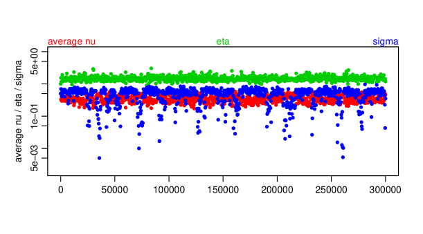
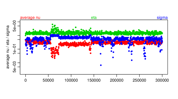
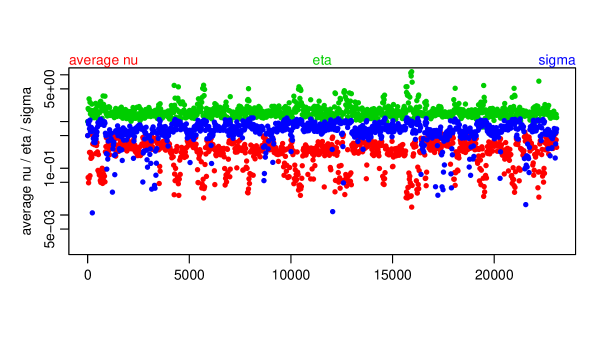
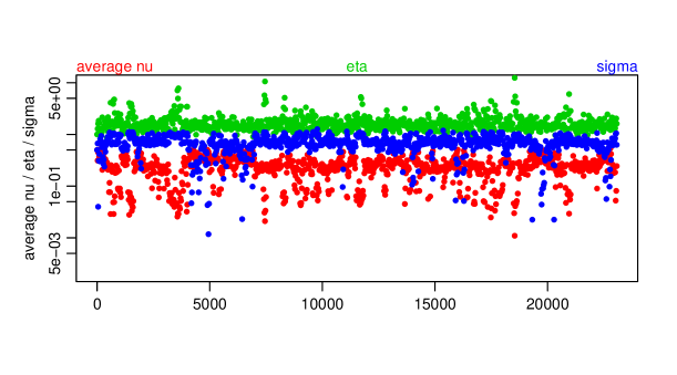
Figure 2 shows results with $s=0.25$ (top) and $s=0.35$ (bottom). The plots show three quantities, on a logarithmic scale, for every 300th iteration from a total of 300,000 Metropolis updates (so that 1000 points are plotted). The quantity shown in red is the average of the $\nu_{h}$ parameters (giving relevances of the covariates), that shown in green is the $\eta$ parameter (the overall scale), and that shown in blue is the $\sigma$ parameter (noise standard deviation).

$s=0.25$:

$s=0.35$:

Figure 2: Runs using Metropolis updates of all parameters at once, with two values for the proposal standard deviation, $s$.

When $s=0.25$, the rejection rate is 87%. From the top plot, it appears that the chain has converged, and is sampling from two modes, characterized by values of $\sigma$ around 0.5, or much smaller values. Movement between these modes occurs fairly infrequently, but an adequate sample appears to have been obtained in 300,000 iterations.

However, the bottom plot shows that this is not the case. The rejection rate here, with $s=0.35$, is high, at 94%, but this chain explores additional modes that were missed in the run with $s=0.25$. The sample from 300,000 iterations is nevertheless far from adequate. Some modes were moved to and from only once in the run, so an accurate estimate of the probality of each mode cannot be obtained.

Metropolis updates that change only one parameter at a time, systematically updating all parameters once per MCMC iteration, perform better. (This is presumably because in the posterior distribution there is fairly low dependence of some parameters on others, so that fairly large changes can sometimes be made to a single parameter.) Updating a $\nu_{h}$ parameter is slow, requiring about the same computation time as an update changing all parameters. However, updates that change only $\eta$, or (if computations are done using eigenvectors) only $\sigma$, will be fast. To allow a fair comparison, the number of iterations done was set so that the number of slow evaluations was 300,000, the same as for the runs with Metropolis updates of all variables at once. To make the comparison as favourable as possible for this method, I assumed that computations are done using eigenvectors, so that both $\eta$ and $\sigma$ are fast variables.

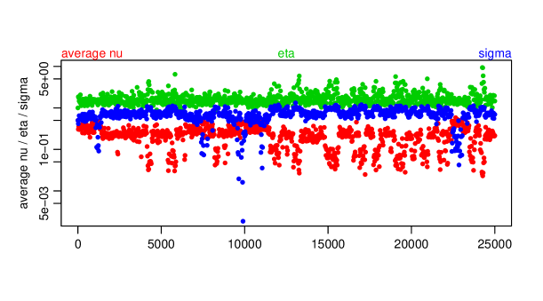
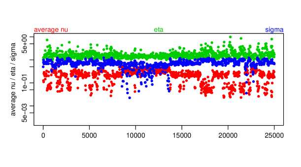
The top plot in Figure 3 shows results using such single-variable Metropolis updates (selected as among the best of runs with various settings that were tried). Here, the proposal standard deviation was 2 for the $\nu_{h}$ parameters, and 0.6 for the $\eta$ and $\sigma$ parameters. (Recall that all parameters are represented by their logs.) The rejection rates for the updates of the variables ranged from 53% to 77%. One can see that sampling is significantly improved, but that some modes are still visited only a few times during the run. One way to try to improve sampling further is to perform additional updates of the fast variables. The bottom plot in Figure 3 shows the results when 49 additional Metropolis updates of the fast variables ($\eta$ and $\sigma$) are done each iteration. This seems to produce little or no improvement on this problem. (However, on some other problems I have tried, extra updates of fast variables do improve sampling.)

Extra:

Figure 3: Runs using Metropolis updates of one parameter at a time, with extra updates of fast parameters for the lower plot.

The time required for a slow evaluation using computations based on the Cholesky decomposition was 0.0081 seconds on the Intel machine, and 0.0661 seconds on the SPARC machine. When using computations based on eigenvectors, a slow evaluation took 0.0128 seconds on the Intel machine, and 0.0886 seconds on the SPARC machine. The ratio of computation time using eigenvectors to computation time using the Cholesky decomposition was therefore 1.58 for the Intel machine and 1.34 for the SPARC machine. Note that this ratio is much smaller than the ratio of times to compute eigenvectors versus the Cholesky decomposition, since times for other operations, such as computing the covariances, are the same for the two methods, and are not negligible in comparison when $n=100$ and $p=12$.

Performance of ensemble MCMC.

I now present the results of using ensemble MCMC methods on this problem. The Metropolis method was used to update the ensemble, so that a direct comparison to the results above can be made, but of course other types of MCMC updates for the ensemble are quite possible. I tried Metropolis updates where the proposals both changed the slow variables and shifted the ensemble of values for fast variables, but keeping the ensemble of fast variables fixed seemed to work as well or better for this problem. Updating only one slow variable at a time worked better than updating all at once.

Accordingly, the results below are for ensemble updates consisting of a sequence of single-variable Metropolis updates for each slow variable in turn, using Gaussian proposals centred at the current value for the variable being updated. After each such sequence of updates, the ensemble was mapped to a single state, and a new ensemble was then generated. (One could keep the same ensemble for many updates, but for this problem that seems undesirable, considering that regenerating the ensemble is relatively cheap.)

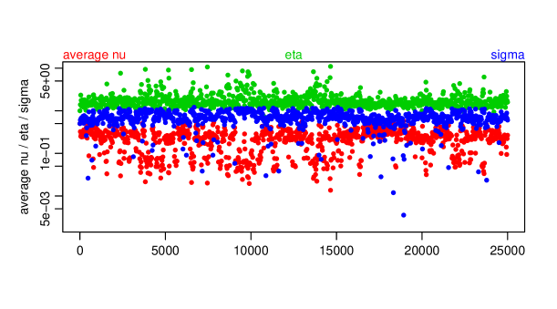
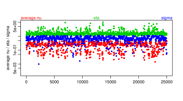
I will first show the results when using computations based on eigenvectors, for which both $\eta$ and $\sigma$ are fast variables. Three ensembles for fast variables were tried — an independent ensemble, with the distribution being the Gaussian prior, an exchangeable ensemble, with the ensemble distribution being Gaussian with standard deviations 0.4 times the prior standard deviations, and a $7\times 7$ grid ensemble, with grid extent chosen uniformly between the prior standard deviation and 1.1 times the prior standard deviation. All ensembles had $K=49$ members. The number of iterations was set so that 300,000 slow evaluations were done, to match the runs above using standard Metropolis updates.

Figure 4 shows the results. Comparing with the results of standard Metropolis in Figure 3, one can see that there is much better movement among the modes, for all three choices of ensemble. The exchangeable and grid ensembles perform slightly better than the independent ensemble. I tried increasing the size of the ensemble to 400, and performing extra updates of the fast variables after mapping back to a single state, but this only slightly improves the sampling (mostly for the independent ensemble).

The time per iteration for these ensemble methods (with $K=49$) was 0.0139 seconds on the Intel machine and 0.0936 seconds on the SPARC machine (very close for all three ensembles). This is slower than standard Metropolis using Cholesky computations by a factor of 1.7 for the Intel machine and 1.4 for the SPARC machine. The gain in sampling efficiency is clearly much larger than this.

Independent:

Exchangeable:

Grid ($7\times 7$):

Figure 4: Runs using ensemble MCMC with computations based on eigenvalues (both $\eta$ and $\sigma$ fast), for three ensembles.

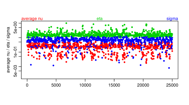
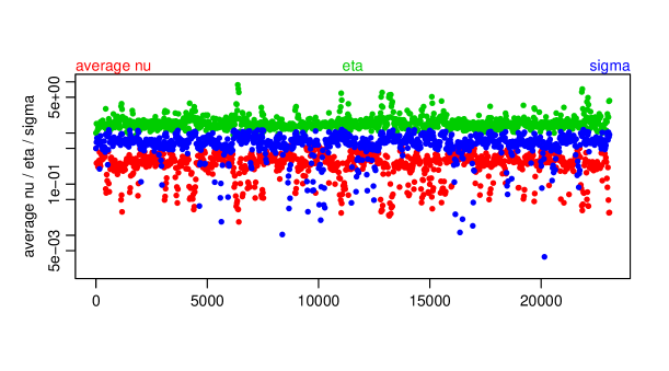
Figure 5 shows the results when computations are based on the Cholesky decomposition, so that only $\eta$ can be a fast variable. Sampling is much better than with standard Metropolis, but not as good as when both $\eta$ and $\sigma$ are fast variables. However, the computation time is lower — 0.0082 seconds per iteration for on the Intel machine, and 0.0666 seconds per iteration on the SPARC machine. These times are only about 1% higher than for standard Metropolis, so use of an ensemble for $\eta$ only is virtually free.

Independent:

Exchangeable:

Grid ($7\times 7$):

Figure 5: Runs using ensemble MCMC with computations based on Cholesky decomposition (only $\eta$ fast), for three ensembles.

Discussion

I will conclude by discussing other possible applications of ensemble MCMC, and its relationship with two previous MCMC methods.

Some other applications.

Bayesian inference problems with fast and slow variables arise in many contexts other than Gaussian process regression models. As mentioned early, many Bayesian models have hyperparameters whose conditional distributions depend only on a fairly small number of parameters, and which are therefore fast compared to parameters that depend on a large set of data points.

For example, in preliminary experiments, I have found a modest benefit from ensemble MCMC for logistic regression models in which the prior for regression coefficients is a $t$ distribution, whose width parameter and degrees of freedom are hyperparameters. When there are $n$ observations and $p$ covariates, recomputing the posterior density after a change only to these hyperparameters takes time proportional to $p$, whereas recomputing the posterior density after the regression coefficients change takes time proportional to $np$ (or to $n$, if only one regression coefficient changes, and suitable intermediate results were retained). The hyperparameters may therefore be seen as fast variables.

In Gaussian process models with latent variables, such as logistic classification models (Neal 1999), the latent variables are all fast compared to the parameters of the covariance function, since recomputing the posterior density for the $n$ latent variables, given the parameters of the covariance function, takes time proportional $n^{2}$, with a small constant factor, once the Cholesky decomposition of their covariance matrix has been found in $n^{3}$ time. Looking at ensemble MCMC for this problem would be interesting, though the high dimensionality of the fast variables may raise additional issues.

MCMC for state-space time series models using embedded Hidden Markov models (Neal, Beal, and Roweis, 2004) can be interpreted as an ensemble MCMC method that maps to the ensemble and then immediately maps back. Looked at this way, one might consider updates to the ensemble before mapping back. Perhaps more promising, though, is to use a huge ensemble of paths defined using an embedded Hidden Markov model when updating the parameters that define the state dynamics.

Relationship to the multiple-try Metropolis method.

A Metropolis update on an ensemble of points as defined in this paper bears some resemblence to a “multiple-try” Metropolis update as defined by Liu, Liang, and Wong (2000) — for both methods, the update is accepted or rejected based on the ratio of two sums of terms over $K$ points, and in certain cases, these sums are of $\pi(x^{(i)})$ for the $K$ points, $x^{(1)},\ldots,x^{(K)}$. In a multiple-try Metropolis update, $K$ points are sampled independently from some proposal distribution conditional on the current point, one of these $K$ proposed points is then selected to be the new point if the proposal is accepted, and a set of $K$ points is then produced by combining the current point with $K\!-\!1$ points sampled independently from the proposal distribution conditional on this selected point. Finally, whether to accept the selected point, or reject it (retaining the current point for another iteration), is decided by a criterion using a ratio of sums of terms for these two sets of $K$ points.

In one simple situation, multiple-try Metropolis is equivalent to mapping from a single point to an ensemble of $K$ points, doing a Metropolis update on this ensemble, and then mapping back to a single point. This equivalence arises when the proposal distribution for multiple-try Metropolis does not actually depend on the current state, in which case it can also be used as an independent ensemble base distribution, and as a proposal distribution for an ensemble update in which new values for all ensemble members are proposed independently. This method will generally not be useful, however, since there is no apparent short-cut for evaluating $\pi(x)$ at the $K$ ensemble points (or $K$ proposed points) in less than $K$ times the computational cost of evaluating $\pi(x)$ at one point.

Applying multiple-try Metropolis usefully to problems with fast and slow variables, as done here for ensemble MCMC, would require that the $K$ proposals conditional on the current state be dependent, since for fast computation they need to all have the same values for the slow variables. Liu, et al. mention the possibility of dependent proposals, but provide details only for a special kind of dependence that is not useful in this context.

In this paper I have emphasized the need for a computational short-cut if ensemble MCMC is to provide a benefit, since otherwise it is hard to see how an ensemble update taking a factor of $K$ more computation time can outperform $K$ ordinary updates. The analogous point regarding multiple-try Metropolis was apparently not appreciated by Liu, et al., as none of the examples in their paper make use of such a short-cut. Accordingly, in all their examples one would expect a multiply-try Metropolis method with $K$ trials to be inferior to simply performing $K$ ordinary Metropolis updates with the same proposal distribution, a comparison which is not presented in their paper.

Relationship to the multiset sampler.

Leman, Chen, and Lavine (2009) proposed a “multiset sampler” which can be seen as a particular example of sampling from an ensemble distribution as in this paper. In their notation, they sample from a distribution for a value $x$ and a multiset of $k$ values for $y$, written as $s=\{y_{1},\ldots,y_{k}\}$. The $y$ values are confined to some bounded region, ${\cal Y}$, which allows a joint density for $x$ and $s$ to be defined as follow:

$$\pi^{*}(x,s) \propto \sum_{j=1}^{k}\pi(x,y_{j})\ \ =\ \ \pi(x)\,\sum_{j=1}^{k}\pi(y_{j}|x)$$ (35)

where $\pi(x,y)$ is the distribution of interest. In some examples, they focus on the marginal $\pi(x)$. Integrating the density above over $y_{1},\ldots,y_{k}$ shows that the marginal $\pi^{*}(x)$ is the same as $\pi(x)$, so that sampling $x$ and $s$ from $\pi^{*}$ will produces a sample of $x$ values from $\pi$. Leman, et al. sample from $\pi^{*}$ by alternating a Metropolis update for just $x$ with with a Metropolis update for $y_{j}$ with $j$ selected randomly from $\{1,\ldots,k\}$.

This $\pi^{*}$ distribution for the multiset sampler is the same as the ensemble distribution that would be obtained using the methods for fast and slow variables in this paper, if $x$ is regarded as slow (and hence written as $x_{1}$ in the notation of this paper), $y$ is regarded as fast (and hence written as $x_{2}$), and in the $\xi$ density used in defining the ensemble base measure, the fast variables in the ensemble are independent, with uniform density over ${\cal Y}$. The density $\rho$ defined by equation (26) then corresponds to the multiset density above.

Leman, et al. do not distinguish between fast and slow variables, however, and hence do not argue that the multiset sampler would be beneficial in such a context. Nor do they assume that there is any other computational short-cut allowing $\pi$ to sometimes be evaluated quickly, thereby reducing the amount of computation needed to evaluate $\pi^{*}$. They instead justify their multiset sampler as allowing $k-1$ of the $y$ values in the multiset to freely explore the region ${\cal Y}$, since the one remaining $y$ value can provide a reasonably high $\pi(x,y)$ and hence also a reasonably high value for $\pi^{*}$.

The development in this paper confirms this picture. With the $\rho$ distribution corresponding to multiset sampling, the mapping $\hat{T}$ will (in the notation of Leman, et al.) go from a single $(x,y)$ pair drawn from $\pi(x,y)$ to an ensemble with $k$ values for $y$, one of which is the original $y$, and the other $k-1$ of which are drawn independently and uniformly from ${\cal Y}$. This is therefore the equilibrium distribuiton of the multiset samplier. The development here also shows that $\pi(x,y)$ can be recovered by applying the $\check{T}$ mapping, which will select a $y$ from the multiset with probabilities proportional to $\pi(x,y)$. This makes the complex calculations in Section 6 of (Leman, et al., 2002) unnecessary.

Unfortunately, it also seems that any benefit of the multiset sampler can be obtained much more simply and efficiently with a Markov chain sampler that randomly chooses between two Metropolis-Hastings updates on the original $\pi$ distribution — one that proposes a new value for $x$ (from some suitable proposal distribution) with $y$ unchanged, and another that proposes a new value for $x$ along with a new value for $y$ that is drawn uniformly from ${\cal Y}$. As is the case as well for ensemble MCMC and multiple-try Metropolis, one should expect that looking at $K$ points at once will produce a benefit only when a short-cut allows $\pi$ for all these points to be computed in less than $K$ times the cost of computing $\pi$ for one point.

References

Earl, D. J. and Deem, M. W. (2005) “Parallel tempering: Theory, applications, and new perspectives”, Physical Chemistry Chemical Physics, vol. 7, pp. 216–222.

Geyer, C. J. (1991) “Markov chain Monte Carlo maximum likelihood”, in E. M. Keramidas (editor), Computing Science and Statistics: Proceedings of the 23rd Symposium on the Interface, pp. 156-163, Interface Foundation. Also available from http://www.stat.umn.edu/$\sim$charlie/.

Gilks, W. R., Roberts, G. O., and George, E. I. (1994) “Adaptive direction sampling”, The Statistician (Journal of the Royal Statistical Society, Series D), vol. 43, pp. 179–189.

Hastings, W. K. (1970) “Monte Carlo sampling methods using Markov chains and their applications”, Biometrika, vol. 57, pp. 97–109.

Leman, S. C., Chen, Y., and Lavine, M. (2009) “The multiset sampler”, Journal of the American Statistical Association, vol. 104, pp. 1029–1041.

Lewis, A. and Bridle, S. (2002) “Cosmological parameters from CMB and other data: A Monte Carlo approach”, Physical Review D, vol. 66, 103511, 16 pages. Also available at http://arxiv.org/abs/astro-ph/0205436. Further notes on MCMC methods for this problem are available at http://cosmologist.info/notes/CosmoMC.pdf.

Liu, J. S., Liang, F., and Wong, W. H. (2000) “The multiple-try method and local optimization in Metropolis sampling”, Journal of the American Statistical Association, vol. 95, pp. 121–134.

Metropolis, N., Rosenbluth, A. W., Rosenbluth, M. N., Teller, A. H., and Teller, E. (1953) “Equation of state calculations by fast computing machines”, Journal of Chemical Physics, vol. 21, pp. 1087–1092.

Neal, R. M. (1999) “Regression and classification using Gaussian process priors” (with discussion), in J. M. Bernardo, et al (editors) Bayesian Statistics 6, Oxford University Press, pp. 475–501.

Neal, R. M. (2004) “Taking bigger Metropolis steps by dragging fast variables”, Technical Report No. 0411, Dept. of Statistics, University of Toronto, 9 pages.

Neal, R. M. (2006) “Constructing efficient MCMC methods using temporary mapping and caching”, talk at Columbia University, Department of Statistics, 11 December 2006. Slides available at http://www.cs.utoronto.ca/$\sim$radford/ftp/cache-map.pdf.

Neal, R. M. (2010) “MCMC using Hamiltonian dynamics”, to appear in the Handbook of Markov Chain Monte Carlo, S. Brooks, A. Gelman, G. Jones, and X.-L. Meng (editors), Chapman & Hall / CRC Press, 51 pages. Also at http://www.cs.toronto.edu/$\sim$radford/ham-mcmc.abstract.html.

Neal, R. M., Beal, M. J., and Roweis, S. T. (2004) “Inferring state sequences for non-linear systems with embedded hidden Markov models”, in S. Thrun, et al (editors), Advances in Neural Information Processing Systems 16 (aka NIPS*2003), MIT Press, 8 pages.

Rasmussen, C. E. and Williams, C. K. I. (2006) Gaussian Processes for Machine Learning, The MIT Press.