The Sunyaev-Zel’dovich Array:
Constraining a New Pressure Profile for Fitting SZE Observations of Galaxy Clusters

Tony Mroczkowski

Professor Amber Miller

Submitted in partial fulfillment of the

requirements for the degree

of Doctor of Philosophy

in the Graduate School of Arts and Sciences.

COLUMBIA UNIVERSITY

2009

©2009

Tony Mroczkowski

All Rights Reserved

Abstract

The Sunyaev-Zel’dovich Array:
Constraining a New Pressure Profile for Fitting SZE Observations of Galaxy Clusters
Tony Mroczkowski

The Sunyaev-Zel’dovich Array (SZA), an eight element interferometer designed to probe the Sunyaev-Zel’dovich effect (SZE) from galaxy clusters, which I helped construct and operate, is described here (Part I). I then use SZA observations to investigate the utility of a new, self-similar pressure profile for fitting SZE observations of galaxy clusters (Part II).

The SZA 30-GHz receiver system probes angular scales $\sim$ 1–5. A model that can accurately describe a cluster’s pressure profile over a correspondingly broad range of radii is therefore required. In the analysis presented here, I fit a 2-parameter, radial pressure profile, derived from simulations and detailed X-ray analysis of relaxed clusters, to SZA observations of three clusters with exceptionally high quality X-ray data. From the joint analysis of the SZE and X-ray data, I derive physical properties of the cluster, such as gas and total mass, gas fraction and the integrated Compton $y$-parameter.

The parameters derived from the joint fit to SZE+X-ray data agree well with a detailed, independent, X-ray-only analysis of these same clusters. When combined with X-ray imaging data, this new pressure profile yields an independent estimate of the electron temperature profile that is in good agreement with spectroscopic X-ray determinations. In addition to yielding relationships between cluster observables and physical cluster properties, this model could prove to be a useful tool in helping to constrain the temperatures of high redshift clusters, for which X-ray spectroscopic data are difficult to obtain.

Acknowledgements

I want to start off by saying this thesis has been an “it takes a village” effort, much more so than simply an individual’s pursuit. I think this is particularly true about those doing instrumentation and experimental astrophysics, unlike those in more traditional student–advisor hierarchies; our experience is necessarily broad in range, and the cultivation of a decent experimentalist requires a great effort by many. Throughout graduate school, I have sought and received advice and guidance from so many people, all of whom are experts in their fields.

First, of course, I would like to thank my advisor Amber Miller, for her guidance and diligence in helping bring this work to fruition. Without her persistence and insistence upon understanding everything on a fundamental level, this work could not possibly have become the complete tome it is today.

I also thank Frits Paerels and Caleb Scharf, who first got me interested in cluster astrophysics, and who were always there when I had questions, doubts, results to share, or just needed someone to put science in perspective.

I thank everyone at the Owens Valley Radio Observatory, all of whom also advised me and helped me keep my sanity. I especially thank David Woody, James Lamb, Ben Reddall, and Dave Hawkins for all their useful direction and for bringing me into their lives at an otherwise remote and alienating place; I know I often was stubborn and unreceptive to their advice, but their persistence has helped to form me into the scientist I am today. I also thank Cecil Patrick, who helped make OVRO fun and gave me plenty of advice on life and cooking; along with Cecil, I also thank his dog Clementine just for being who she is. And of course I thank Dianne Shirley and the girls – Xena, Katie, Aukee, and Minnie – for all the wild times in Bishop, California.

I thank everyone in the Sunyaev-Zel’dovich Array (SZA) Collaboration. I especially thank Marshall Joy and Max Bonamente for helping me understand the many levels of cluster analysis required for this work. I thank Daisuke Nagai for all his patient conversations that guided me in testing these analysis routines on simulated clusters and helped produce relevant models for fitting cluster data. I thank Erik Leitch for all his useful discussions that helped me understand radio interferometry, and for all his help with computers. I thank John Carlstrom, who always raised good questions and was fun to work with in the field. And finally, I thank my fellow students in the SZA – particularly Matthew Sharp and Stephen Muchovej – who helped make this more fun than it often should have been.

And while those in science have been so crucial to the completion of this work, I especially thank those who were there for me just because they like me. Foremost, I thank my wife, Natalia Holstein, who has put up with a lot (I’m sorry I have to be out of town so much to do this stuff). This would not have been possible without her love, support, and welcome distractions. I thank her mother too, for being curious and brave enough to ask questions about my work. I thank my friends – particularly Brian Cleary, Nathaniel Stern, Dave Spiegel, and Paul Kim – who kept things interesting and convinced me I was smart enough to get this done. And I thank my family, who helped make me what I am today.

Last, but not least,

I would like to thank Nina for being the only one who never questioned the value of this work, and for always waiting patiently by my desk throughout.

Chapter 0 Introduction

“What’s so amazing that keeps us stargazing? What do we think we might see?” – Kermit the Frog (The Rainbow Connection, written by Paul Williams and Kenneth Ascher)

1 Clusters of Galaxies

The detailed expansion history of the Universe and the growth of large scale structure are two of the most important topics in cosmology. Clusters of galaxies are the largest gravitationally-bound systems in the Universe, and thus provide a unique handle on cosmic expansion and structure formation. Measurements of the growth of structure, traceable using large cluster surveys, provide critical clues to the nature and abundance of dark matter and dark energy.

At the time of this writing, a low density, cold dark matter (CDM) cosmology, dominated by a dark energy or cosmological constant ($\Lambda$) component, is heavily favored. This is called $\Lambda$CDM cosmology, where ‘$\Lambda$’ refers to dark energy’s contribution, expressed as $\Omega_{\Lambda}$, to the total energy density of the Universe, $\Omega$. Cold dark matter is a form of non-baryonic matter travelling much slower than the speed of light, which – along with the baryonic component $\Omega_{\rm b}$ – provides matter’s energy density contribution $\Omega_{\rm M}$. In general, any quantity $\Omega_{x}$ is the ratio of $x$’s energy density to the critical energy density it would take to close the Universe.

$\Lambda$CDM cosmology started to become the favored cosmology in the 1990’s, when it displaced the then-favored – and now inappropriately-named – Standard Cold Dark Matter (SCDM) picture of the Universe. SCDM holds that $\Omega_{\rm M}=\Omega_{\text{tot}}=1$ ($\Omega_{\Lambda}=0$). $\Lambda$CDM cosmology reconciles two results that cannot be resolved in the SCDM paradigm: the flatness of the Universe combined with the low value for the universal matter density $\Omega_{\rm M}$.

In the mid-1990’s, X-ray gas mass measurements began to demonstrate that $\Omega_{\rm M}<1$. Because galaxy clusters collapse out of representatively large, comoving volumes of the Universe ($\sim 10$ Mpc), we assume their baryonic/dark matter ratio approaches the universal value. Using X-ray measurements of galaxy clusters, one can obtain both the hot gas mass ($M_{\mbox{\scriptsize gas}}$) and an estimate of the cluster total mass $M_{\mbox{\scriptsize tot}}$, and use these to compute the gas mass fraction $\mbox{$f_{\mbox{\scriptsize gas}}$}\equiv\mbox{$M_{\mbox{\scriptsize gas}}$}/\mbox{$M_{\mbox{\scriptsize tot}}$}$. Provided that the bulk of a cluster’s baryons are in the hot gas probed by X-ray observations, we can approximately equate the gas mass fraction $\mbox{$f_{\mbox{\scriptsize gas}}$}\approx\Omega_{\text{gas}}/\Omega_{\rm M}\sim\Omega_{\text{b}}/\Omega_{\rm M}$ (within a factor of $\sim 2$, this is well-supported by the simulations).

The combination of $f_{\mbox{\scriptsize gas}}$ measurements with constraints from Cosmic Microwave Background (CMB) measurements and Big Bang Nucleosynthesis (BBN) predictions yields an estimate for $\Omega_{\rm M}$. Since CMB measurements, coupled with BBN theory, independently constrain $\Omega_{\text{b}}h^{2}$ (where $h$ is the local Hubble constant divided by $100~{}\rm km~{}s^{-1}~{}Mpc^{-1}$), one can use cluster gas fraction measurements to approximately constrain $\Omega_{\rm M}$. By accounting for the composition of the Coma cluster – adding up the observable mass in the hot gas and optically luminous stars – White et al. (1993) argued that the measurements implied a low value for $\Omega_{\rm M}$ in this way. Later, David et al. (1995) applied this method to many more clusters observed by ROSAT, and used this to estimate that $\Omega_{\rm M}\sim$ 0.1–0.2.

Furthermore, X-ray cluster surveys – such as those provided by the ROSAT All-Sky Survey (RASS) and the Wide Angle ROSAT Pointed Survey (WARPS) – provided independent indications that we live in a low density universe with $\Omega_{\rm M}\sim$ 0.2–0.3. This low density was inferred from the lack of strong cluster number evolution, which would have been seen if $\Omega_{\rm M}=1$ (see, e.g. Mushotzky & Scharf 1997), as the matter density strongly affects when clusters form (see, e.g. Holder et al. 2000; Haiman et al. 2001, and references therein).

Whilst cluster measurements consistently implied we live in a low density universe, direct evidence for dark energy was provided by those who set out to measure the deceleration of the Universe’s expansion, using type Ia supernovae (SNIa) as “standard candles” (objects with a known luminosity). Surprisingly, their measurements indicated that the expansion of Universe is accelerating (Riess et al. 1998), implying it is dominated by some form of dark energy. Soon after, measurements of the CMB made by the BOOMERanG, TOCO, and MAXIMA strongly constrained the Universe to be spatially flat, a result that has been confirmed by WMAP and other CMB measurements since. With no curvature component ($\Omega_{\rm k}=0$), “flatness” means that the sum of the angles within a triangle is $180^{\circ}$, and that $\Omega_{\rm M}+\Omega_{\Lambda}=1$.

With strong evidence now in place for $\Lambda$CDM, and many more recent results confirming this, a “concordance cosmology” with $\Omega_{\Lambda}=0.7$, $\Omega_{\rm M}=0.3$, and $\Omega_{\rm k}=0$ can be defined. This cosmology is assumed for most of the results presented in this thesis, and is in agreement with the parameters published in the first year results of the Wilkinson Microwave Anisotropy Probe (Spergel et al. 2003, WMAP), which jointly fit data from a number of independent tests (e.g. their own and finer scale probes of the CMB, weak lensing, cluster counts, galactic velocity field, and HST’s Key Project) described in Spergel et al. (2003). Defining a “concordance cosmology” provides a convenient framework for both observers and theorists. As cosmological constraints are refined, any results assuming this cosmology can be scaled to reflect the updated parameters.

Recently, a number of studies have used clusters alone to constrain the dark energy component of the Universe (see Allen et al. 2004; LaRoque et al. 2006; Allen et al. 2007; Vikhlinin et al. 2008, and references therein). This is done primarily using X-ray measurements of the intracluster medium (ICM), the hot ($\gtrsim 10^{7}~{}\rm K$) gas that comprises the majority of the baryons in a galaxy cluster. Assuming a theoretically-motivated functional form for the gas fraction, one can solve for the cosmological parameters that force the data to fit the expected $\mbox{$f_{\mbox{\scriptsize gas}}$}(z)$ evolution for redshift $z$.

In this thesis, I explore the joint constraints provided by two independent probes of the ICM, using these to measure $f_{\mbox{\scriptsize gas}}$, $M_{\mbox{\scriptsize gas}}$, $M_{\mbox{\scriptsize tot}}$, and other cluster astrophysical properties. In the next section, I describe the primary tool used here to constrain the properties of the ICM – the Sunyaev-Zel’dovich effect.

2 The Sunyaev-Zel’dovich Effect

Figure 1: Image adapted from van Speybroeck (1999).

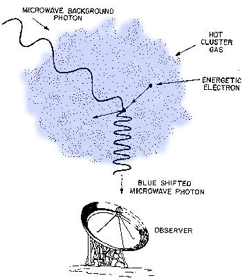
The Sunyaev-Zel’dovich effect (SZE) is a unique probe of the hot gas in clusters, since it does not depend on emission processes, unlike X-ray emission or the broad majority of luminous astrophysical processes routinely measured by astronomers. The SZE arises by inverse Compton scattering of CMB photons off the hot electrons in the ICM (depicted schematically in Fig. 1). This leaves a spectral signature on the CMB that is independent of redshift, since at higher redshifts the CMB is both denser in photon number and less redshifted in energy.

There are two separable components to the Sunyaev-Zel’dovich effect: the kinetic SZ effect, or KSZ, due to the line-of-sight proper motions of clusters, and the thermal SZ effect (TSZ, simply called ‘SZE’ in the chapters that follow). I do not discuss the KSZ here, since we could not measure it with the Sunyaev-Zel’dovich Array (SZA, the instrument presented in this thesis; see Chapter 1). The thermal SZE is measurable as a spectral distortion of the CMB, computed

$$\frac{\Delta T}{\mbox{$T_{\mbox{\tiny CMB}}$}}=f(x)\,y,$$ (1)

where $\Delta T$ is the temperature distortion of the CMB, which has temperature $T_{\mbox{\tiny CMB}}$, $y$ is called the “Compton $y$ parameter” and is integrated along the line of sight, and $f(x)$ (given in Eqs. 4 and 5) contains the SZE frequency dependence.

The line-of-sight Compton $y$ parameter is computed

$$y=\frac{k_{B}\,\mbox{$\sigma_{\mbox{\tiny T}}$}}{m_{e}c^{2}}\int\!n_{e}(\ell)\,T_{e}(\ell)\,d\ell,$$ (2)

where $k_{B}$ is Boltzmann’s constant, $\sigma_{\mbox{\tiny T}}$ is the Thomson scattering cross-section of the electron, $m_{e}$ is the mass of an electron, $c$ is the speed of light, and $n_{e}(\ell)$ and $T_{e}(\ell)$ are the electron density and temperature along sight line $\ell$. The Compton $y$ parameter has a linear dependence on electron pressure $P_{e}$ when the ideal gas law, $P_{e}=k_{B}\,n_{e}\,T_{e}$, is assumed:

$$y=\frac{\mbox{$\sigma_{\mbox{\tiny T}}$}}{m_{e}c^{2}}\int\!P_{e}(\ell)\,d\ell.$$ (3)

The classical, non-relativistic frequency dependence $f(x)$ of the SZE is

$$f(x)=x\left(\frac{e^{x}+1}{e^{x}-1}\right)-4$$ (4)

where the dimensionless frequency $x$ is

$$x=h\nu/k_{B}\mbox{$T_{\mbox{\tiny CMB}}$}.$$ (5)

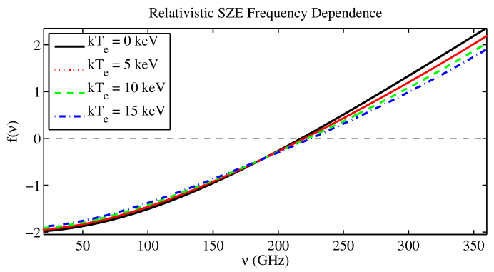
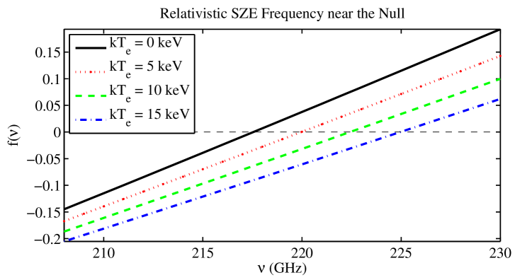
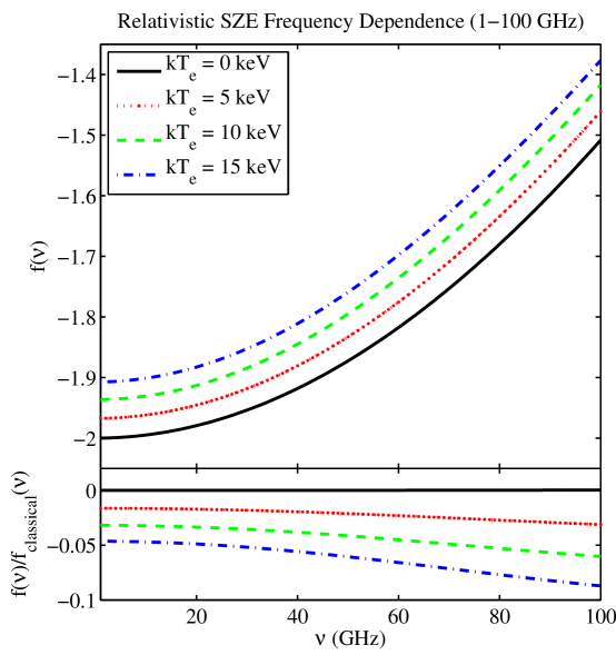
Here $h$ is Planck’s constant, and $\nu$ is the frequency of the observation. The classical spectral dependence $f(x)$ given in Eq. 4, and relativistic corrections to it – necessary due to the high thermal velocities of electrons in the ICM – are plotted in the upper panel of Fig. 2 over a broad range of frequencies. Here I used the calculations of Itoh et al. (1998), which correct the SZE $f(x)$ out to fifth-order. The SZE decrement $\lesssim 218~{}\rm GHz$ becomes an increment at $\gtrsim 218~{}\rm GHz$. A detail of this crossover is shown in the lower panel of Fig. 2, which shows that the relativistic velocities of the electrons, due to the cluster’s temperature, shift the precise location of SZE null. Finally, Fig. 3 shows a detail of the SZE decrement at the frequencies the SZA can probe.

Figure 2: SZE spectral dependence $f(\nu)$, plotted as a function of frequency (see Eq. 5). The upper panel shows $f(\nu)$ over a broad range of frequencies, while the lower panel shows a detail of the null in the SZE spectrum. The relativistically-corrected $f(\nu)$ for a cluster with temperature $kT_{e}=0~{}\rm keV$ (black, solid line) reduces precisely to the classical frequency dependence (Eq. 4), since electrons with no temperature are not moving at relativistic random velocities. The other lines show how the relativistically-corrected $f(\nu)$ departs from the classical behavior for higher temperature electrons. The relativistic corrections to $f(\nu)$ shown here are computed out to fifth-order using the equations provided in Itoh et al. (1998). The classical SZE spectrum has a null at $\nu\approx$ 217.5 GHz, above which the SZE signal becomes an increment. Higher temperature electrons require relativistic corrections (Itoh et al. 1998) to the classical SZE frequency dependence, which shift the null to higher frequencies. A high temperature cluster would have a non-negligible thermal SZ effect at the classical null (217.5 GHz).

Figure 3: SZE frequency dependence below 100 GHz. See Fig. 2 for caption. Below the null (see lower panel of Fig. 2), we often use the term “SZE decrement” to refer to the strength of the thermal SZ effect, which is negative at low frequencies. The lower panel shows the fractional deviation from the classical SZE for clusters at higher temperatures, due to the relativistic electron velocities in the ICM. Treating the thermal SZE at 30 GHz from a massive 10 keV cluster as classical introduces a $\approx-3.6\%$ bias in quantities derived from the SZE fits (i.e. the line-of-sight electron pressure in Eq. 2 would be underestimated by this amount, since the strength of the SZE would be overestimated by the classical calculation).

3 Interferometry Overview

Monochromatic light from an arbitrarily-shaped, spatially-incoherent aperture propagates via Fraunhofer diffraction to become the spatial Fourier transform of the light’s intensity pattern, after traveling a distance many times its wavelength. Radio astronomical interferometry takes advantage of this simple fact, where the astronomical source serves as the arbitrary aperture. An interferometric array measures the Fourier transform of the source’s spatial intensity distribution, probing angular scales $\lambda/d^{\prime}$ (in radians) for wavelength $\lambda$ and projected baseline separation $d^{\prime}$ (see Fig. 4).

Figure 4: Example baseline formed by a pair of antennae. The dish separation is $d$, while the projected baseline as seen by the source is $d^{\prime}$. The distance to the source (represented by a cloud) is labeled $R_{ff}$. Note the scale of the broken lines, representing this astronomical distance $R_{ff}$, is not accurate; in reality, the lines of sight are nearly parallel and point at the same location on the source. The time delay $T$ is equal to the difference in distances to the source, from each antenna, divided by the speed of light $c$. By delaying the signal measured by the antenna on the right by time $T$, we ensure that the same astronomical wavefront is used in the correlation of the two signals. Tracking an astronomical source requires both the physical pointing of each antenna toward the source in the far field, and the implementation of instrumental delays ($T$) that ensure each antenna measures the same wave front as the Earth rotates.

1 Criteria and Assumptions for Interferometry

The conditions necessary to take advantage of astronomical interferometry constitute the “van Cittert-Zernike theorem” (see Thompson et al. 2001, for a derivation and many further details). I summarize the necessary criteria here:

• The source must be in the far field, meaning that its distance $R_{ff}\gg(d^{\prime})^{2}/\lambda$ (illustrated in Fig. 4), where $d^{\prime}$ is the longest projected baseline in the array for a given observation, and $\lambda$ is the wavelength at which the observation is performed. A large distance is essential for statistically independent emission (or scattering events, in the case of the SZE) from the source to become coherent plane waves. For the Sunyaev-Zel’dovich Array, this means we must observe sources more than 360 km away, a condition met by any astronomically interesting source. In meeting the far field condition, for a sufficiently narrow band, we can treat incoming light from the source as a series of plane waves.

• As a corollary to the above, we assume there are no sources in the near field, so we are only observing sources in the far field.

• The source must be spatially incoherent, meaning that two arbitrary points within the source must not have statistically correlated emission. Since two points within a source are physically separated and entirely independent, emission from these two points will not in general be coherently emitted.

We also take advantage of one more approximation: the small angle approximation. While this is not necessary for the van Cittert-Zernike theorem, it simplifies the analysis of interferometric observations, as it allow us to treat the data as a 2-D Fourier transform (discussed in the next section, §2).

As I discuss later in this section, the largest radial scales probed by the SZA are on the order of $\sim 5\arcmin$ ($1.45\times 10^{-3}$ radians). The small angle approximation is therefore well-justified for single, pointed observations made with the SZA (as opposed to mosaicked observations). We therefore treat the spatial intensity pattern of the source as if it were truly in a plane perpendicular to the line of sight. We call this the “image plane,” and justify this by pointing out that the sources we observe are far enough away that the distance to any part of the source is negligibly different from the radial distance to the source’s center.

At a given instant in time, all antennae must measure a single, monochromatic wavefront for the astronomical signals to be correlated. The signals are measured within spectral channels (a “channel” is a smaller range of frequencies within some band) that are small compared to the central frequency of each band, assuring each signal is approximately monochromatic. To ensure the condition that we are measuring a single plane wave front, the differing distances from each antenna to the source are corrected by adding (computationally) an adjustable time delay to each antenna’s signal. This adjustable delay is the difference in path lengths from the astronomical source to each antenna, divided by the speed of light (labeled $T$ in Fig. 4). The path length $cT$ changes throughout the course of an observation, as the source traverses the sky.

In radio interferometry, computing and applying the proper delays to the signal from each antenna, as the Earth moves, is called “fringe tracking.” The Cartesian location $(x,y)=(0,0)$ (typically north-south and east-west angular offsets) is assigned to the point in the sky called the “pointing center.” Mechanical tracking keeps this point (e.g. a cluster’s center) in the center of each antenna’s primary beam; the pointing center is also the “phase center” for the observation, since the adjustable delays $T$ are computed in order to precisely compensate for the different distances to this point. These differing distances are based simply on the geometry illustrated in Fig. 4.

2 Probing Sources in Fourier Space (u,v-space)

Figure 5: SZA u,v-space coverage of CL1226.9+3332 (12:26:58.0, +33:32:45.0), a cluster that passes near zenith for the SZA (the SZA’s latitude is $\sim 37^{\circ}$N). Each blue point represents a data point’s u,v-space location, using frequency independent units of $k\lambda$ (distance divided by wavelength, divided by 1000). Note that there are 2 groupings of points: those $\sim$ 0.35–1.3 k$\lambda$ from the center, due to the short baselines of the compact inner array, and those $\sim$ 3–7.5 k$\lambda$ from the center, due to the long baselines formed with the outer antennae (i.e. each baseline formed with Antennae 6 or 7; the antenna layout of the SZA is shown in Fig. 7). The SZA was designed to provide this broad, uniform coverage in u,v-space on the shorter baselines, while simultaneously providing higher resolution coverage with longer baselines. The data locations in u,v-space exhibit inversion symmetry (i.e. $(u,v)=-(u,v)$) because the visibilities are the transform of real data in image space. The visibilities therefore exhibit Hermitian symmetry (i.e. $V_{\nu}(u,v)=V_{\nu}^{*}(-u,-v)$ in Eq. 6).

Figure 6: SZA u,v-space coverage of A1835 (14:01:02.03, +02:52:41.71), a low declination cluster (the SZA’s latitude is $\sim 37^{\circ}$N). See Fig. 5 for caption. Note that the coverage provided by the inner baselines is nearly as complete as that in Fig. 5. The coverage on longer baselines, used to constrain the fluxes of sources known to be point-like (using independent radio surveys), is less complete. If a source is truly point-like, the u,v-space coverage provided by the long baselines does not need to be complete to remove it, since a point source has the same magnitude of flux over all of u,v-space (we generally do not use the SZA to determine whether a source is point-like, and need only constrain its flux. See §2 for more details about modeling unresolved radio sources.).

Figure 7: SZA Antenna Locations. Antenna 2 is the reference antenna, and is therefore located at the origin. Antennae 6 & 7 provide 13 long baselines (between each other and paired with each of the six inner antennae). These long baselines probe small scales, thus aiding point source subtraction. Figures 5 & 6 show the u,v-space coverage of two sources observed with this array configuration.

Figure 8: Radial distribution of scales probed in u,v-space ($\sqrt{u^{2}+v^{2}}$), for coverage shown in Fig. 5. The distribution is extremely bimodal due to the short ($\sim$ 0.35–1.3 k$\lambda$, plotted in green) and long ($\sim$ 3–7.5 k$\lambda$, plotted in blue) baselines of the SZA (shown in Fig. 7).

Figure 9: Radial distribution of scales probed in u,v-space for coverage shown in Fig. 6. See Fig. 8 for details. Because of the low declination of A1835, the projected baselines for this observation are shorter, on average, than those for CL1226 (Fig. 8).

In the context of astronomical interferometry, Fourier space is often referred to as “u,v-space,” since $u$ and $v$ are the Fourier conjugates of image space coordinates $x$ and $y$. When calibrated against an astronomical source of known flux, an interferometric array’s output can be expressed as the flux (in Janskies) at each point probed in u,v-space, for each frequency probed by the instrument. For a given integration time (typically $\sim$ 20 sec for the SZA), each baseline and band of the radio interferometric array produces one binned point in u,v-space, called a “visibility.” The visibilities behave collectively as a Fourier transform of the spatial intensity pattern $I_{\nu}(x,y)$ (flux per unit solid angle) at frequency $\nu$, and is calculated (Thompson et al. 2001):

$$V_{\nu}(u,v)=\int\!\int A_{\nu}(x,y)\,I_{\nu}(x,y)\,\frac{e^{-j2\pi(ux+vy)}}{\sqrt{1-x^{2}-y^{2}}}\,dx\,dy.$$ (6)

Here $A_{\nu}(x,y)$ is the spatial sensitivity of each antenna, the central lobe of which is called the primary beam (illustrated in Fig. 2). Each antenna’s beam was mapped by Ryan Hennessy and Mike Loh, and was found to be well-approximated by a single, circularly-symmetric Gaussian with a half-power radius of $\sim 4.9\arcmin$. Because our observations are on the scales of arcminutes, we can make the approximation that $\sqrt{1-x^{2}-y^{2}}\approx 1$, where $x$ and $y$ in are radians. Doing this, Eq. 6 simplifies to the 2-D Fourier transform of the spatial intensity pattern multiplied by the beam:

$$V_{\nu}(u,v)=\int\!\int A_{\nu}(x,y)\,I_{\nu}(x,y)\,{e^{-j2\pi(ux+vy)}}dx\,dy.$$ (7)

Figure 10: SZA u,v-space coverage of CL1226.9+3332, combining observations from both the 30-GHz (blue) and 90-GHz (magenta) instruments. See Fig. 5 for caption. Observations with the SZA using the 90-GHz receivers (see §1), thus probe finer scales (larger u,v-scales) than the 30-GHz system for the same array configuration.

Figure 11: Radial distribution of scales probed in u,v-space ($\sqrt{u^{2}+v^{2}}$), for coverage shown in Fig. 10. The $\sim$ 1.3–3 k$\lambda$ gap in the coverage at 30 GHz (shown in blue) is filled in by performing complementary observations at 90 GHz (show in magenta). For a given array configuration and observation length, the 90-GHz u,v-coverage can be obtained (approximately) by multiplying each u,v coordinate in the 30-GHz u,v-coverage by $\sim 3$.

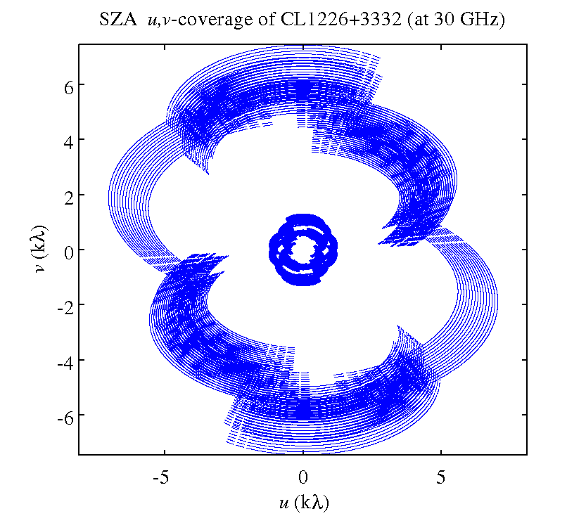
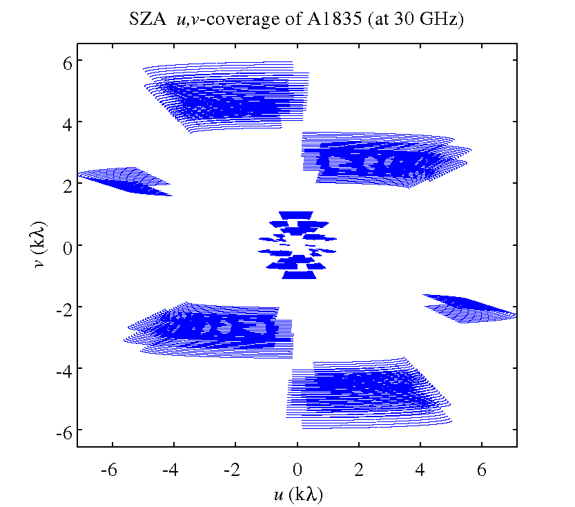
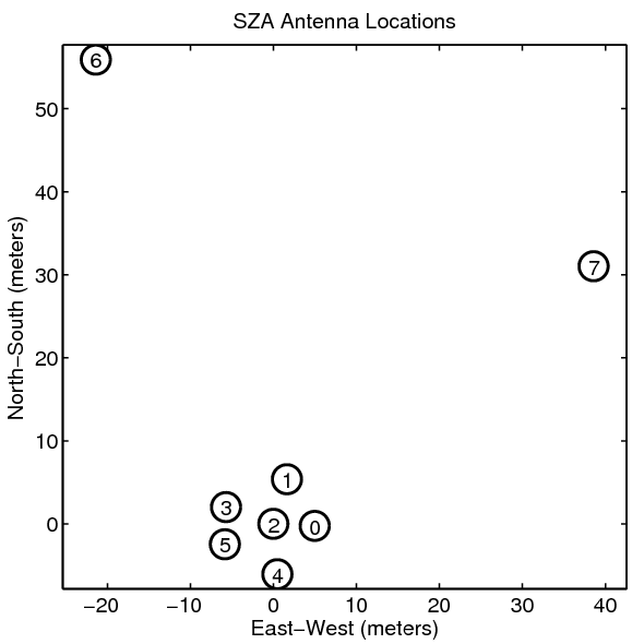
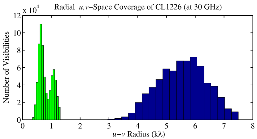
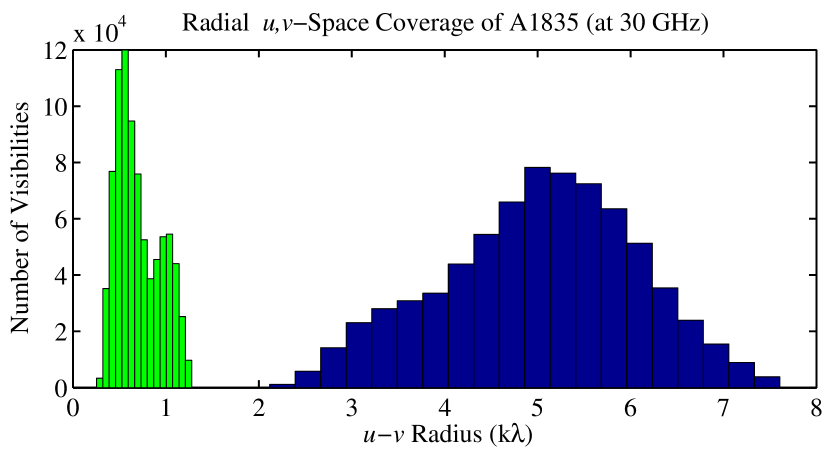
Figures 5 & 6 show the u,v-space coverage of the SZA interferometer during two typical cluster observations. This coverage was provided using the array configuration shown in Fig. 7, performing observations with the 30-GHz receivers. Figures 8 & 9 respectively show the distributions of u,v-radii probed by the u,v-spacings plotted in Figs. 5 & 6. The incompleteness of this coverage necessarily means information on those scales not probed is missing; an interferometer filters information on scales it cannot access. In fact, the SZA was designed specifically to probe cluster (arcminute) scales. Since the scales to which we are sensitive are proportional to $\lambda/d$ in radians, long baselines of a 30-GHz SZA observation ($\sim$ 3–7.5 k$\lambda$) probe angular scales $\theta\propto\lambda/d=$ 0.46–1.15$\arcmin$, while short baselines of that same observation ($\sim$ 0.35–1.3 k$\lambda$) probe angular scales $\theta\propto\lambda/d=$ 2.6–9.8$\arcmin$. The SZA 30-GHz system is essentially not sensitive to radial scales larger than $\sim 5\arcmin$ (the 90-GHz system, discussed below, probes scales one-third these sizes). In this way, the SZA isolates the small ($\Delta T$ in Eq. 1 typically peaks $\sim 10$ mK) cluster signal from the relatively large background (e.g. the atmospheric and instrumental noise discussed in §1, as well as the 2.73 K primary CMB).

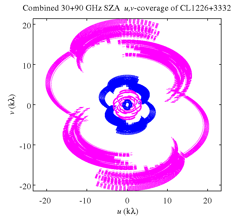
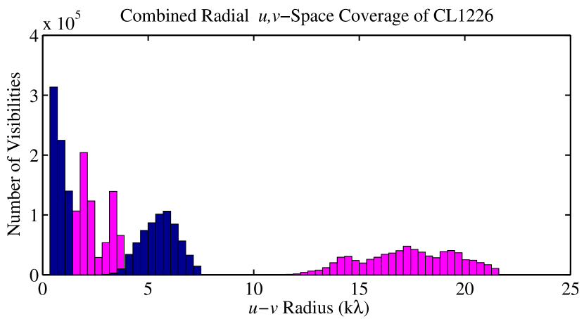
By including SZA observations performed using the 90-GHz receivers, using the same array configuration shown in Fig. 7, the gap at $\sim$ 1.3–3 k$\lambda$ in the u,v-coverage at 30 GHz can be filled. Since the wavelenth is $\sim$ 3 times shorter at 90 GHz than it is at 30 GHz, each baseline at 90 GHz is effectively $\sim$ 3 times longer in $\lambda$ (number of wavelengths). The combined 30+90 GHz coverage is shown in Fig. 10, while the corresponding histogram of radial u,v-scales probed by combining the observations is shown in Fig. 11. The short baselines of the 90-GHz system, ranging $\sim$ 1.2–3.8 k$\lambda$, constrain cluster signals in the intermediate angular scales $\theta\propto\lambda/d=$ 0.9–2.9$\arcmin$.

4 X-ray imaging of Galaxy clusters

In this thesis, I use X-ray imaging data taken with the Chandra X-ray Observatory, extending the work of Reese et al. (2002), LaRoque et al. (2006), Bonamente et al. (2006), and others to combine X-ray imaging data with new SZE data taken with the SZA.

Figure 12: The effective collecting area of the Chandra primary mirror, as a function of photon energy. This response dominates the energy response of the instrument. It also reduces the plasma emissivity that Chandra effectively sees from a high temperature plasma (Fig. 13).

At X-ray wavelengths, emission from a cluster is predominantly due to thermal processes that occur in the same gas that produces the SZE. The two thermal processes by which the ICM emits X-rays are bremsstrahlung and line emission (see, e.g. Longair 1998; Sarazin 1988), both of which depend on collisions between pairs of particles within the gas (i.e. two particles are involved in the emission process). The X-ray emission therefore scales as number density-squared. In contrast, the SZE depends linearly upon electron pressure (Eq. 2). These two ways of probing the ICM therefore complement each other.

X-ray imaging data are sensitive to the surface brightness $S_{X}$ (in $\rm cts~{}arcmin^{-2}~{}s^{-1}$):

$$S_{X}=\frac{1}{4\pi(1+z)^{4}}\!\int\!\!n_{e}(\ell)^{2}\mbox{$\Lambda_{ee}$}(T_{e}(\ell),Z)\,d\ell$$ (8)

where $n_{e}(\ell)$ and $T_{e}(\ell)$ are the electron density and temperature along sight line $\ell$, $\Lambda_{ee}(T_{e},Z)$ (in $\rm cts~{}cm^{5}~{}s^{-1}$) is the X-ray emissivity measured by the instrument within the energy band used for the observation, $z$ is the cluster’s redshift, and $Z$ is the plasma’s metallicity. Metallicity accounts for elements heavier than helium, where $Z_{\odot}\equiv 1$ is defined to be the elemental abundance measured in the solar atmosphere, and the abundances in a cluster are measured relative to the solar abundance (see §1 for a more detailed discussion of elemental abundances and metallicity). For $T\gtrsim 3~{}\rm keV$, the X-ray emissivity of the plasma depends weakly on temperature. Before accounting for the instrument’s response (discussed below), $\Lambda_{ee}(T_{e})\propto T^{1/2}$ since the X-ray emission is bremsstrahlung-dominated at these energies.

Figure 13: The X-ray emissivity of a cluster plasma at redshift $z=0.25$, redshifted to local photon energy range 0.7–7.0 keV, as measured by Chandra (using the instrument’s effective area shown in Figure 12). The plasma emissivity was computed using the plasma model of Raymond & Smith (1977) for a range of cluster temperatures and metallicities (see §1). The effective emissivity we measure is reduced by Chandra’s efficiency, which declines for photon energies $>4~{}\rm keV$ (see Fig. 12). For plasma temperatures $\lesssim 2~{}\rm keV$, the cluster X-ray emission is dominated by lines produced by elements heavier than helium. Since Chandra’s sensitivity peaks at energies between 1–2 keV, the effective emissivity of a plasma with temperature $\sim 1~{}\rm keV$ has a strong metallicity dependence (compare at $\sim 1~{}\rm keV$ the effective emissivity of a plasma with metallicity $Z=0.9$, versus that with $Z=0.1$).

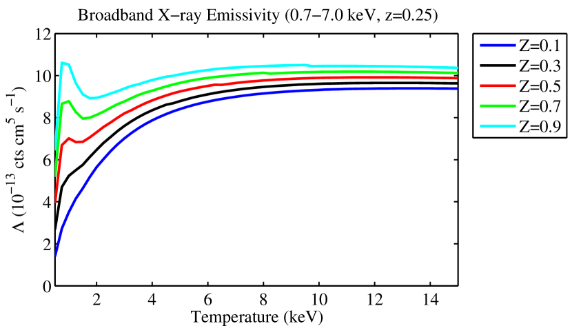
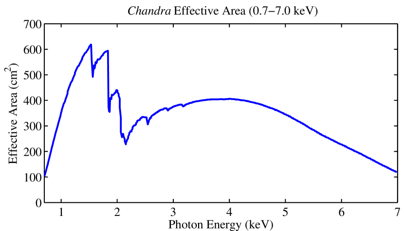
In addition to the already-weak temperature dependence of the plasma emissivity, the “effective emissivity” of the plasma as measured by Chandra is reduced by the instrument efficiency, which declines for photon energies $>4~{}\rm keV$. Chandra’s efficiency is dominated by the “effective area” of the primary mirror for a photon of a given wavelength; the typical energy response of the Chandra ACIS-I CCD is plotted in Fig. 12. The effective emissivity measured by Chandra in a given energy band accounts for the instrument’s efficiency at that energy, and is plotted in Figure 13 for a range of plasma temperatures and metallicities for a plasma at $z=0.25$. To obtain the total number of counts per pixel in an exposure, the result of Eq. 8 must be multiplied by the exposure time and the field of view (in arcmin²) of a pixel.

5 Structure of the Thesis

I describe the SZA instrumentation in Chapter 1, and discuss how we addressed challenges encountered during SZA commissioning observations in Chapter 2. In Chapter 3, I discuss SZA data calibration and the final data product used in cluster analyses.

In Chapter 4, I discuss the joint modeling of SZE+X-ray data, and present the new models used. I also discuss our data fitting routine and how we derive cluster parameters of interest from the models. In Chapter 5, I apply the models to real observations and discuss the results. Finally, in Chapter 8, I present my conclusions and some ideas for extensions to these modeling techniques.

Part 1 Instrumentation and Data Reduction

Chapter 1 The Sunyaev-Zel’dovich Array

1 Overview of the Sunyaev-Zel’dovich Array

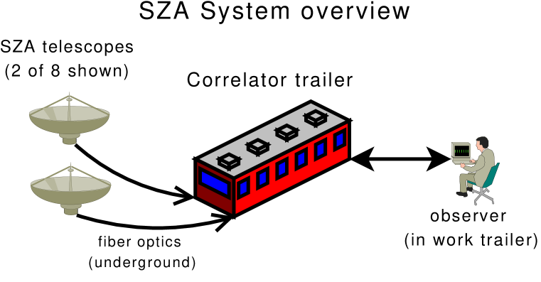
The Sunyaev-Zel’dovich Array (SZA), an interferometer composed of eight 3.5 meter telescopes, is located at the Owens Valley Radio Observatory, in Big Pine, California. Its coordinates are $37^{\circ}14\arcsec 02\arcsec$ latitude and $118^{\circ}16\arcsec 56\arcsec$ longitude, and it is at an altitude of 1222 meters above sea level. The Owens Valley is a desert, and therefore provides suitable atmospheric conditions for performing centimeter and millimeter-wave observations for most of the year.

The SZA has a digital correlator with 8 GHz of bandwidth (see Hawkins et al. 2004, for details on the correlator), and each antenna is equipped with two wideband receiver systems, capable of observing from 27-36 GHz (in the Ka band, hereafter referred to as the “30-GHz” band) and from 85-115 GHz (in the W band, referred to as the “90-GHz” band). See Fig. 1 for a broad overview of the SZA system. The large, 8-GHz receiver and correlator bandwidth provides the SZA with the high sensitivity required to detect rapidly cluster signals. This wide bandwidth also provides the ability to probe a wide range of u,v-space (Fourier conjugate of image space) simultaneously, meaning it is sensitive to a wider range of angular scales than a comparable instrument with a smaller bandwidth.

The SZA receivers contain high electron mobility transistors (HEMT) for high gain, low noise amplification of incoming signals. The 30-GHz receivers contain the same HEMT amplifiers that were in the Degree Arcminute-Scale Interferometer (DASI) (see Leitch et al. 2005), in the same configuration used for the OVRO/BIMA SZE receivers (see Carlstrom et al. 1998, 2000). The 90-GHz receivers utilize HEMTs implemented through monolithic microwave integrated circuit (MMIC) technology, which integrates four HEMTs into each MMIC block.

Figure 1: SZA System Overview. The SZA has eight 3.5 m antennae that communicate via fiber optic connections to equipment in a general-purpose utility trailer, which is referred to as the “Correlator Trailer.” This trailer houses the downconverter, correlator, control system computer, and other electronics common to the system. The observer commands the control system using an interface programmed by Erik Leitch that utilizes the SSH (secure shell) protocol.

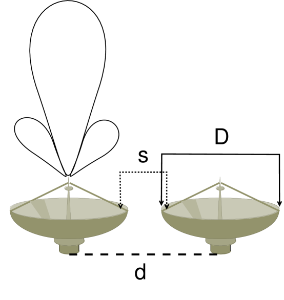
The SZA was designed to detect and probe clusters at intermediate and higher ($z\gtrsim 0.2$) redshifts. The relatively small (3.5 m) primary mirrors and their short focal lengths (see §2) provide two advantages for SZE observations of clusters: a large primary beam, which scales as $\lambda/D$ for observational wavelength $\lambda$ and primary mirror size $D$, and the ability to closely pack the antennae without resulting in inter-antenna collisions. The full width half maximum (FWHM) size of the truncated Gaussian primary beam, where the sensitivity falls to -3 dB of the peak, is $\approx 10.7\arcmin$ at the center of the 30 GHz band. This is necessary so that objects on arcminute scales, such as clusters are intermediate redshifts, are relatively unattenuated by the primary beam. The scales probed by an interferometer are determined by the projected separation distance $d$ (the distance between the centers of two antennae as seen from the source), and scale as $\lambda/d$. Because the SZA routinely observes clusters all the way to the antenna shadowing limit of 3.7 meters (i.e. the projected antenna spacing is nearly as small as the dish size), it can in principle probe radial angular scales larger than $\sim 4.8\arcmin$ at the central frequency of 30.938 GHz. This is because, for a projected baseline of length $d$, there are points on the primary mirrors separated by distances $s\in[d-D,d+D]$ that are not entirely attenuated by the primary beam (see Fig. 2).

Figure 2: Detail of a pair of antennae. The primary mirror diameter is $D$ (solid line). The center-to-center antenna separation (long dashed line) is $d$, which when looking at zenith (as depicted here) is also the projected baseline length. Separation $s$ (short dashed line) is a distance between two arbitrary points on the primaries separated by less than $D$. A cross-sectional representation of the main and secondary lobes of the antenna sensitivity pattern is shown above the left antenna, where the first sidelobe (secondary lobe) is greatly exaggerated in scale; It was, in reality, measured (by James Lamb) to be -25 dB ($10^{-2.5}\approx 1/316^{\text{th}}$) less than the sensitivity at the center of the primary beam (main lobe).

Figure 3: Photo of the inner 6 telescopes (Antennae 0–5) of the SZA. Photo is taken from the northeast (roughly along Baseline 2-7; see Fig. 7). Antenna 5 is behind Antennae 1 and 3, and Antenna 4 is behind Antenna 0.

Figure 4: Photo of the outer 2 telescopes of the SZA (Antennae 6 & 7, see 7), taken while standing near the inner array. Antenna 6 is shown in the left panel, and Antenna 7 is shown in the right panel.

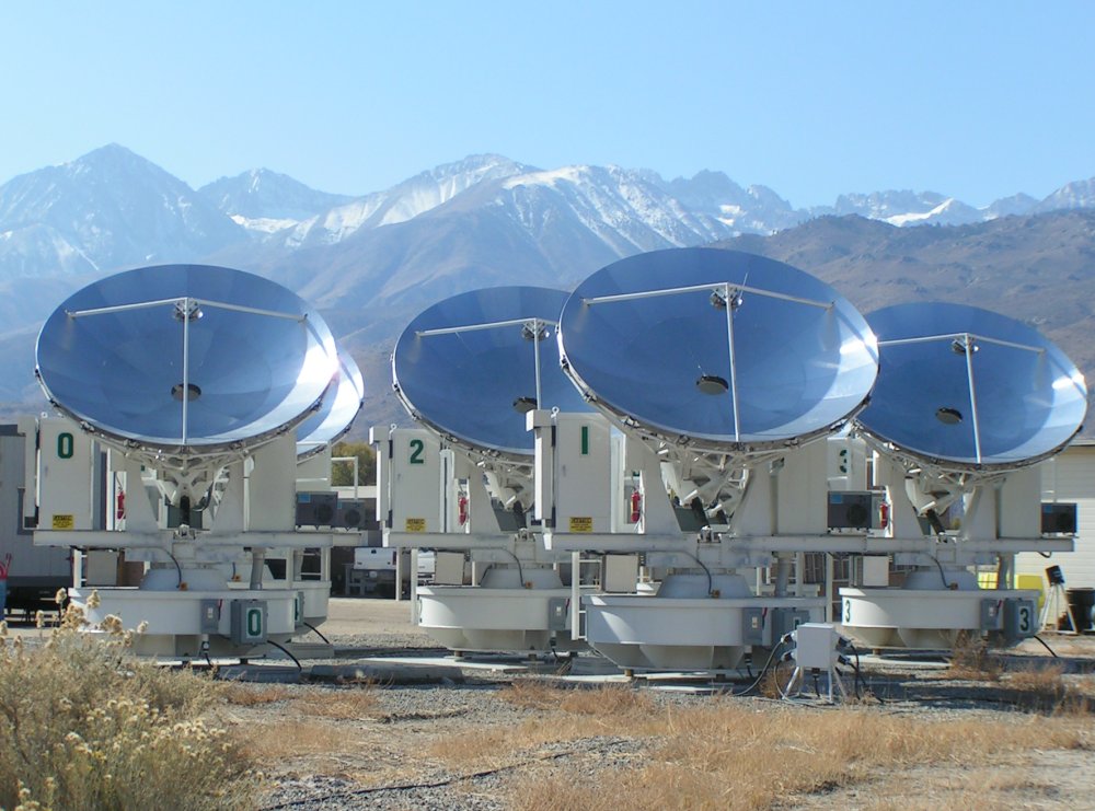
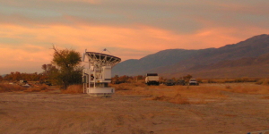
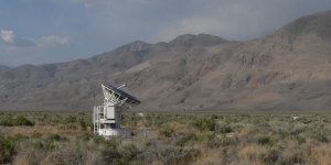
Six of the eight SZA antennae, forming fifteen baselines, comprise the closely-packed “inner array,” which is sensitive to $\approx$ 1-5scales. The inner array is shown in Fig. 3. Two outer antennae (Fig. 4), which are identical to the inner six, form thirteen more baselines (i.e. one baseline between the two outer antennae, and six baselines formed between each outer antenna with each of the inner six; see Fig. 7). These outer antennae provide the ability to fit simultaneously any unresolved ($\lesssim 20\arcsec$) radio sources (hereafter “point sources”) in the cluster field, which could otherwise mask the SZE decrement at 30 GHz.

As discussed in §3, when observing an astronomical source, in addition to the physical pointing of each antenna that keeps the source in the main lobe of the antenna beam pattern (see Fig. 2), the delays necessary for fringe tracking must be computed. Fringe tracking corrects the phases for the instantaneous projected baseline changes due to geometry, as the source moves through the sky, relative to the array (see Fig. 4). Phase changes can also be due to effects that are more difficult to calculate. For example, variations in the lengths of the fiber optics and cables that carry the signals can change the phases of the signals from each antenna. Phase shifts due to properties of the electronics themselves can also act as path length differences (at a particular frequency). These instrumental phase effects are particularly sensitive to temperature fluctuations.

In this chapter, I provide an overview of the components that comprise the SZA. Emphasis is placed on thermal and mechanical aspects of the instrument, as this was the focus of the instrumentation component of this thesis. Thermal stability and the consequences of poor thermal regulation are discussed as appropriate.

2 Telescope Optics

The antennae of the SZA are designed as on-axis, altitude-azimuth telescopes with small primary mirrors that have short focal lengths (see Fig. 5). Their design allows for a compact array configuration with the antennae spaced as close as $1.2D$, where $D$ is the diameter of the primary, without ever colliding. The panels of the primary mirrors were machined by Jerry Forcier of Forcier Mechanics using a conventional, computer numeric controlled (CNC) mill, programmable using standard computer-aided design/machining (CAD/CAM) code. Since the mill operates in standard Cartesian coordinates, the machining process provided the mirrors with a scalloped surface. The tool and toolpath used to machine the primaries were chosen so that the scalloping scatters higher frequency light (e.g. IR and optical), which would otherwise damage the instrument if, for example, the sun were focused on the receiver. The surface was measured by Marshall Joy to have an rms roughness of $25~{}{\rm\mu m}$, meeting the design requirements necessary for the 1.3 mm upgrade the SZA may see as part of CARMA (see e.g. Woody et al. 2004; Scott & Pound 2006).

Figure 5: Overview of the SZA antenna optical design. The primary (light blue) and secondary (red) mirrors are on-axis reflectors. The tertiary mirror (silver) selects the 30 or 90-GHz receiver within the receiver cryostat (dark green). The receiver cryostat is located within the larger receiver enclosure box (not shown). Image adapted from David Woody.

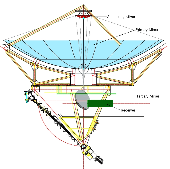
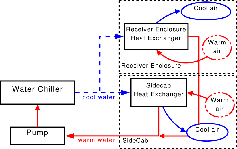
The secondary mirrors are convex paraboloids which slow the focus before it enters the receiver enclosure. The receiver enclosure is simply a large, weather-proof, thermally-regulated box that holds the receiver cryostats, the back-end electronics (which are further enclosed in a smaller, thermally-regulated electronics box), the tertiary mirror, an ambient calibrator load, and various support electronics. In the fall and spring, the receiver enclosure is cooled by air circulating through closed-cycle air/air heat-exchangers. In the summer, the enclosure is cooled by a refrigerated water/antifreeze solution, which is pumped through a closed liquid/air heat-exchanger (similar to a car radiator, containing refrigerated fluid) between the air in the box and the chilled fluid (see Figure 6). In the winter, the box is heated by ceramic, AC-powered heaters. In addition to protecting equipment from the elements (e.g. dust, harsh sunlight, and rain), the receiver enclosure serves as the first step in achieving thermal stability, and its stability helps reduce expansion and contraction of the section of fiber optics closest to the receiver.

Figure 6: Flow chart of the closed-loop chiller system. Warm water is pumped through a cool chiller reservoir. The chilled water continues on to the sidecab, which is a weather-tight equipment rack containing the antenna computers, the motion control system and servos, and electronics power supplies, and to the receiver enclosure (described in the text). The warm air is blown across the fins of the heat-exchangers, through which the cool water is circulated, removing heat. The chilled air returned to the surrounding sidecab or receiver box, as appropriate, where it cools the electronics. The water, now warm, returns to the pump input, where it is recirculated through the system.

The signal enters the receiver enclosure through a microwave transparent (has a very small absorption/reflection coefficient – less than a few percent), weather-proof window made of $75~{}{\rm\mu m}$ mylar and 1-inch thick zotefoam (a nitrogen-filled, polyethylene foam). Zotefoam, a commercially-available foam used in housing construction, was chosen because it is highly transparent at microwave frequencies. It is a closed-cell foam that does not permit air or water diffusion, and is very robust both chemically and mechanically. This mylar layer in front of the zotefoam of the receiver enclosure’s window provides an additional – and easily replaceable – layer of protection from dust and water, which cling to the porous surface of the zotefoam. Thin mylar, such as that used for the windows, is also microwave-transparent.

The next mirror in the optical path – directly after the window to the receiver enclosure – is an adjustable tertiary mirror: a concave, off-axis paraboloid that bends the optical path by $90^{\circ}$ into the receiver. This programmable tertiary selects the receiver into which the signal is focused.

3 Receivers

1 Receiver Noise Considerations

The primary goals of receiver design are the attainment of high gain and low noise. We characterize noise in terms of the “receiver noise temperature” $T_{\rm rx}$, which is derived in this section.

The power emitted in the Rayleigh-Jeans tail of a blackbody is approximately linearly proportional to its temperature. For two thermal sources at temperatures $T_{\rm hot}$ and $T_{\rm cold}$, we measure output powers $P_{\rm hot}$ and $P_{\rm cold}$, which are linearly proportional to the source temperatures as long as the gain of the receiver system also remains linear over that range. Our measurement includes an additional, constant amount of power due to the noise in the receiver, which can be attributed to a hypothetical thermal source at temperature $T_{\rm rx}$. This receiver noise temperature therefore characterizes the output power that we would measure in the absence of any input power. We define the receiver $y$ factor (the ratio of the measured output powers):

$$y\equiv\frac{P_{\rm hot}}{P_{\rm cold}}=\frac{T_{\rm hot}+T_{\rm rx}}{T_{\rm cold}+T_{\rm rx}}$$ (1)

Solving for $T_{\rm rx}$, we have:

$$T_{\rm rx}=\frac{T_{\rm hot}-y~{}\!T_{\rm cold}}{y-1}$$ (2)

Contributions to $T_{\rm rx}$ can include noise from the receiver cryostat windows, amplifiers, mixers, waveguides, and the feed horns. These contributions are all affected by the physical temperatures of the components.

The total contribution $T_{\rm rx}$ from the receiver to the noise is calculated in terms of each component’s gain $G$ (which can be less than unity) for $n$ stages:

$$T_{\rm rx}=T_{1}+\frac{T_{2}}{G_{1}}+\frac{T_{3}}{G_{1}G_{2}}+\ldots+\frac{T_{n}}{G_{1}G_{2}\ldots G_{n-1}}$$ (3)

In Eq. 3, the noise due to each successive stage is reduced by the combination of gains before it ($G_{1}\cdot G_{2}\cdot\ldots\cdot G_{n-1}$). The first components in a receiver – the window and the feed horn – are chosen to have low loss and be well-matched to the incoming signal, respectively, in order to reduce their noise contributions. In addition to being well-matched to the incoming signal, the feed horns are kept at low temperature, which reduces their noise contribution. The first stage amplifier typically dominates the overall receiver noise temperature $T_{\rm rx}$. We therefore optimize the system to have a high-gain, low-noise amplifier at the first (and at every, if possible) stage of amplification. Higher current, higher noise amplifier stages follow this stage, providing most of the overall amplification of each receiver system.

For the overall noise contribution to a signal from a telescope – including contributions from the back-end electronics, the atmosphere, optical elements in the signal path to the receiver, and of course the noise from the receiver itself – we define the system temperature $T_{\rm sys}$, where the $y$ factor in Eq. 1 is instead measured at the output of the entire system, and $T_{\rm sys}$ is scaled to above the Earth’s atmosphere (i.e. we include the noise contribution of the atmosphere with the instrumental noise in one term; see §4.). The dominant contributions – in order of importance – to the total system temperature $T_{\rm sys}$ are therefore the receiver noise $T_{\rm rx}$, the sky ($\sim$ 10–20 K at zenith), noise scattered from the ground (which is called “spillover,” and is $\sim 4$ K at very low elevations, which we avoid when observing), loss due to the windows in the optical path, poor coupling with the feed horn, and the noise contribution from first stage of the HEMT or MMIC amplifier.

2 Measuring $T_{\rm rx}$

In the laboratory, we used a piece of Eccosorb^® as a “hot load” (a thermal load with $T=T_{\text{hot}}$ in Eq. 2). The “cold load” (a thermal load with $T=T_{\text{cold}}$ in Eq. 2) was another piece of Eccosorb^® at liquid nitrogen’s (abbreviated $LN_{2}$) boiling point ($\approx$ 77 K at 1 atmosphere of pressure). This is achieved by keeping the blackbody material in a bath of $LN_{2}$, and removing it for the measurement (for only a few seconds, so it retains evaporating $LN_{2}$ throughout the measurement).

On the SZA telescopes, the hot load is a mechanized version of the same ambient blackbody used in the lab, mounted to the front of the receiver cryostat. However, a true cold load with an $LN_{2}$ bath would be impractical in our system. Instead, careful tracking of atmospheric temperature and humidity allow a model to be developed for the power contribution from the sky, and therefore the sky serves as the “cold load” for calibration purposes.

Under ideal observational conditions the atmospheric contribution to the noise scales as the optical depth. The optical depth scales roughly as $\sec(\theta)$ for angle $\theta$ measured from zenith. This $\sec(\theta)$ dependence only holds if assuming a plane-parallel atmosphere; this is a gross simplification, and the true calculation used in data calibration does not make this assumption. To reduce the noise contribution from the atmosphere, we typically observe sources with elevations $\gtrsim 30^{\circ}$ above the horizon.

3 Receiver RF Components

Figure 7: Photo of Receiver Cryostat Electronics test setup. Items 1–10 are components of the 90-GHz receiver, and 11–16 are components of the 30-GHz receiver. See §3 for details on each RF component. The stages of the refrigerator (17 & 18) are discussed in §4. The copper strapping attached to 17 is not the final version.

Figure 8: 90-GHz receiver block diagram, courtesy of Amber Miller. See the photo in Fig. 7, which shows these components: 1. 90-GHz Feedhorn. 2. Circular Polarizer & Circular-to-Rectangular Transition. 3. 1^st MMIC HEMT Amplifier. 4. Isolator. 5. 2^nd MMIC HEMT Amplifier, Isolator, & High Pass Filter (under bracket). 6. W-band Mixer. 7. Waveguide for the incoming signal from 90 GHz tunable LO, the bias-tuned Gunn. 8. IF Amplifier. 9. Bandpass Filter. 10. K-band Mixer.

Figure 9: 30-GHz receiver block diagram, courtesy of Amber Miller. See the photo in Fig. 7, which shows these components: 11. 30-GHz Feedhorn. 12. Circular Polarizer & Circular-to-Rectangular Transition. 13. HEMT amplifier (under a mount). 14. Isolator. 15. 27 GHz High Pass Filter. 16. Mixer. The IF Amplifier in this figure was later moved outside the receiver.

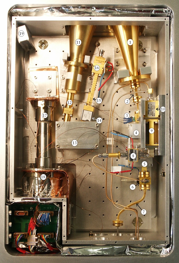
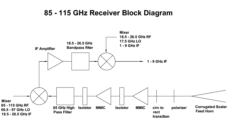
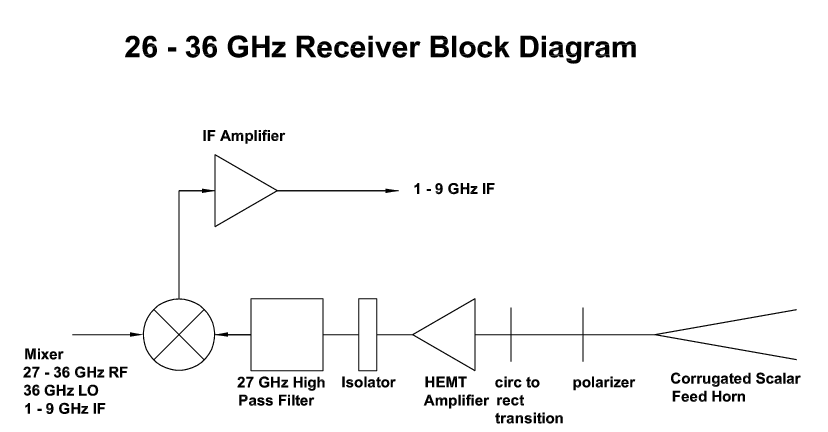
Within the cryostat there are two complete, independent receiver systems (see photo in Fig. 7). These receivers are capable of observing at sky frequencies 27–36 GHz (the “30-GHz receiver”) and 85–115 GHz (the “90-GHz receiver”). Each receiver (see Figures 9 and 8) begins with a corrugated feed horn (#1 and #11 in Fig. 7) that couples the incoming signal to a circular polarizer (#2 and #12 in Fig. 7). A circular-to-rectangular transition, which unfortunately rejects one linear polarization, couples the circular polarizer to a rectangular (linearly polarized) waveguide. The components that follow – starting with the HEMT and MMIC amplifiers (#3 and #13 in Fig. 7) – are specific to each receiver system. I present the 30-GHz receiver first, but note that it is similar in design to the 90-GHz system.

30-GHz Receiver RF Components

In the 30-GHz receiver, a single HEMT amplifier with four stages (i.e. four discrete HEMTs) amplifies the signal. An isolator (#14 in Fig. 7), which reduces reflections coming back from the filter, follows the HEMT amplifier. Next, a high-pass filter (#15 in Fig. 7) eliminates unwanted signals below 27 GHz, and helps to determine the range of the intermediate frequency (IF) signal, which is the sky signal mixed down to 1–9 GHz (see §1 for a description of the SZA downconversion scheme). We refer to the 1–9 GHz band as the “IF band,” and provide the corresponding sky frequencies of each band within the IF band (see Table 1, §1). The IF band is the band in which all the back-end electronics (§4) common to both the 30 and 90-GHz receivers work. A mixer (#16 in Fig. 7), using a 35.938 GHz local oscillator (LO) as its reference, mixes sky frequencies 26.938–34.938 GHz down to the 1–9 GHz IF band (the LO is discussed in §1, while the full downconversion from sky to IF bands is discussed in §1).

The high pass filter determines the upper end of the IF band by attenuating signals below 27 GHz. The high filter attenuates unwanted harmonics related to the LO, since the LO is actually the 4th harmonic of an 8.972 GHz oscillator (discussed in §4) mixed with a 50 MHz phase reference frequency, and other harmonics of the 8.972 GHz oscillator can be present in the system. I discuss RF contamination – and how we eliminated it – in §1.

90-GHz Receiver RF Components

The 90-GHz receiver (see Fig. 8) is similar to the 30-GHz receiver, with a few exceptions. Notably, it has two MMIC amplifiers (#3 and #5 in Fig. 7), each of which contains four HEMTs (i.e. four stages), since these higher-frequency MMIC HEMTs have less gain than their 30-GHz counterparts. The MMICs are separated by an isolator (#4 in Fig. 7), which reduces coupling between the gain stages. Feedback between the stages could otherwise lead to oscillations, since coupling from reflections is a form of positive feedback (which is intrinsically unstable).

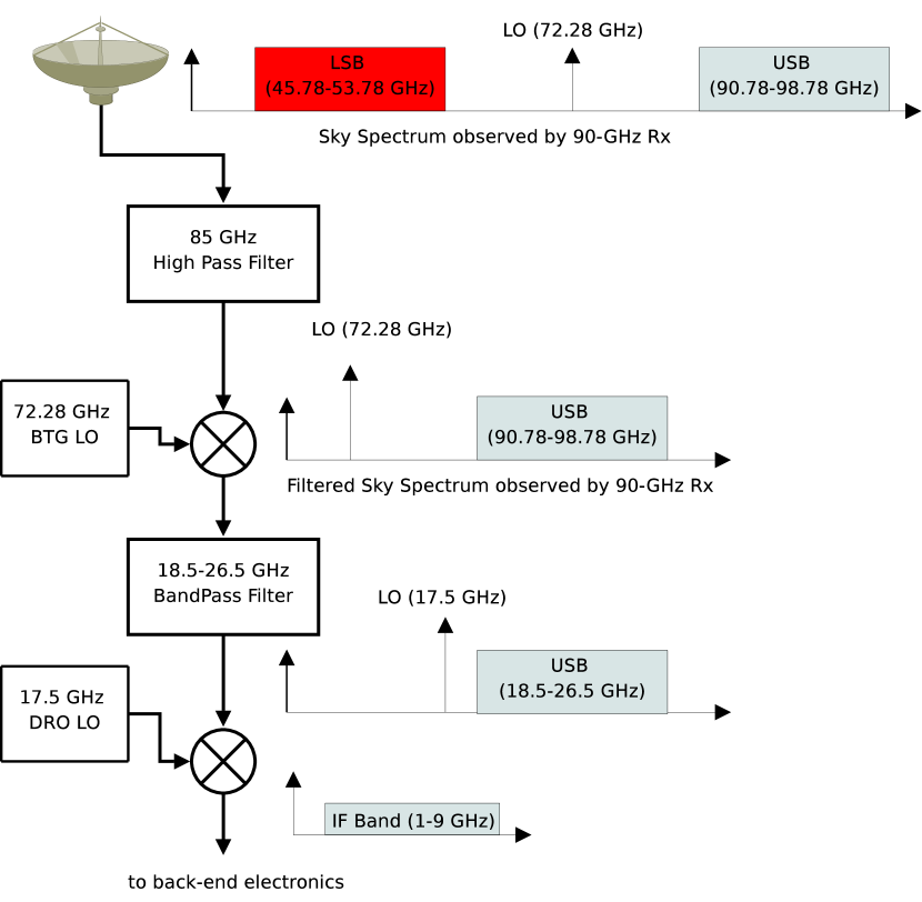
There are two mixers in the 90-GHz system. The first (#6 in Fig. 7) mixes the sky signal with a tunable LO that, along with an 18.5–26.5 GHz bandpass filter (#9 in Fig. 7), selects the range of observable sky frequencies for the 90-GHz receiver. The second mixer (#10 in Fig. 7), using a fixed-frequency, 17.5 GHz dielectronic resonant oscillator (DRO), brings the signal down to the 1–9 GHz IF band. An additional IF amplifier (#8 in Fig. 7) is present in the 90-GHz system for two reasons – the MMIC HEMTs have less overall gain than their 30-GHz counterparts, and mixers are lossy components that split the input signal power among the output mixing products. Since the output of the 90-GHz receiver is handled by the same electronics setup as that which handles the 30-GHz receiver’s output, the two systems need to have comparable output power levels.

4 Thermal Considerations for the Receivers

The signal enters the receiver cryostat through a zotefoam and mylar window. The RF components in the receiver are sensitive to temperature, and therefore must be kept cool (11-20 K) to reduce noise. This necessitates the placement of the amplifiers and other noise-sensitive components in a vacuum-sealed cryostat.

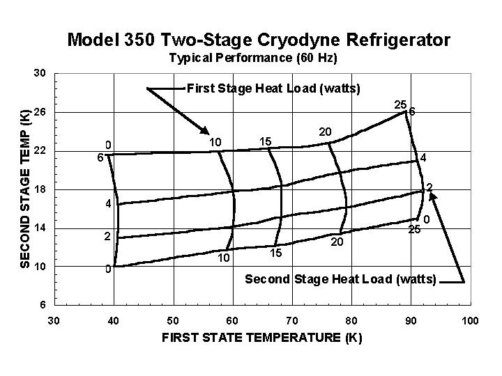
The cryostat is cooled by a CTI-cryogenics Model 350 Cryodyne refrigerator, which offers two stages of cooling: the first (#8 in Fig. 10) is a higher power, warmer stage that runs at $\sim$ 55 K under a load of about 10 W, and the second (#7 in Fig. 10) is a lower power, cooler stage that runs at $\sim$ 12 K when the load is about 1 W (see Fig. 11). The cryostat is therefore built in two stages as well: A warmer radiation shield, made of aluminum ($\gtrsim 90\%$ reflectivity in the microwave and far infrared, where the thermal emission at $\lesssim 100$ K peaks), and a cooler stage within the shield, where the most sensitive components of the system are mounted.

Figure 10: Receiver Cryostat Thermal test setup. Test hard-soldered strapping (4) on the second stage of the cold head (7) is shown. The long copper shims (5), used to increase the thermal conductivity between the RF components and the cold head, were replaced with more flexible, nickel-plated, braided-copper straps. Also in the photo: 1 is the zotefoam window, within the window holder (2). The cryostat case is labeled 3 (the upper lid, which is not shown, mates here to make a vacuum seal). The cold plate, to which most of the RF components are mounted, is 6. The first stage of the refrigerator head is 8. The radiation shield is 9, and the exposed part of the refrigerator head is 10. Mylar blanketing can be seen filling the space between the cryostat case and the radiation shield.

Figure 11: The load curve for the CTI-cryogenics Model 350 Cryodyne refrigerator. Figure from Brooks Automation, the company that now owns Helix Technology CTI-Cryogenics.

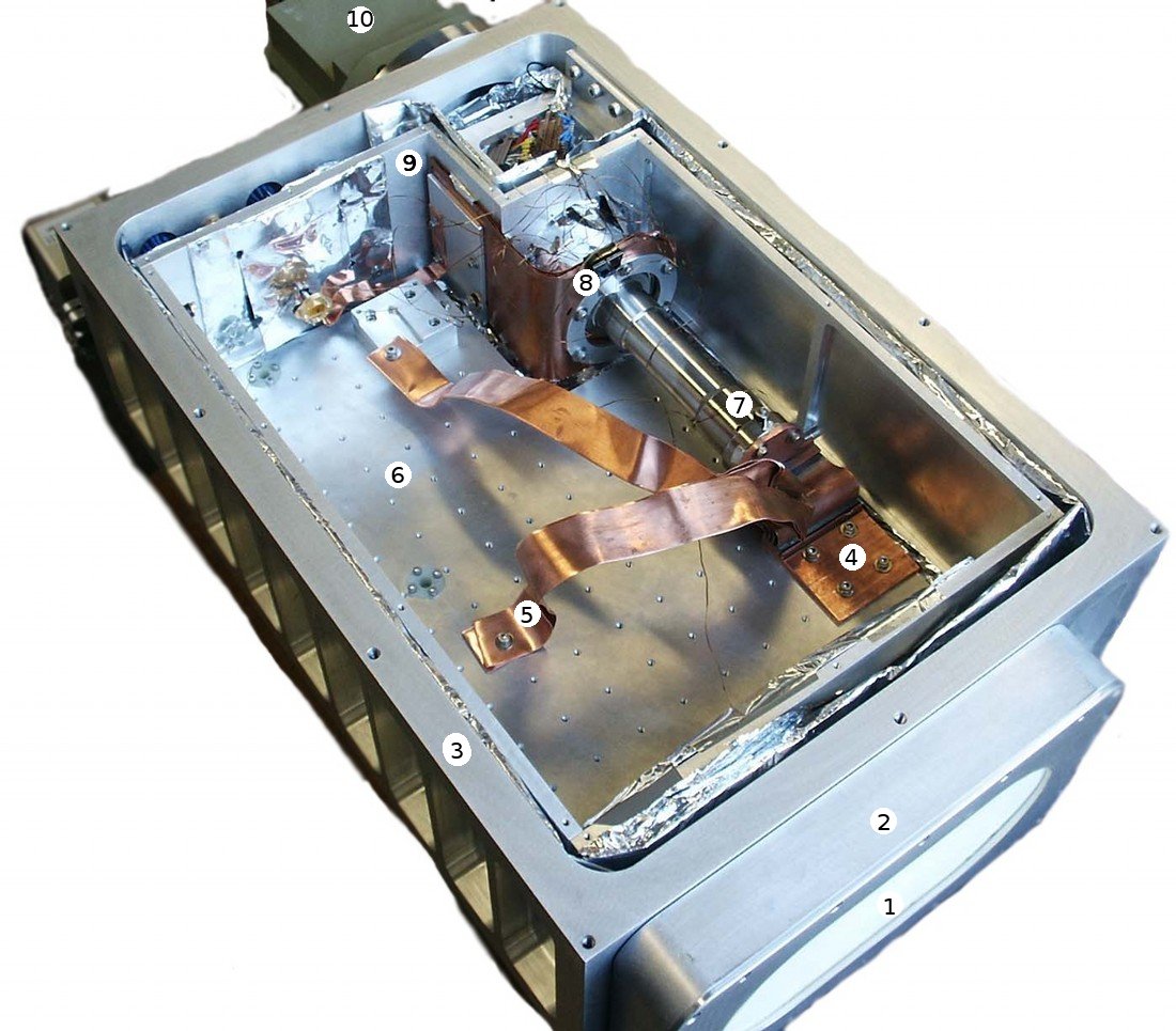
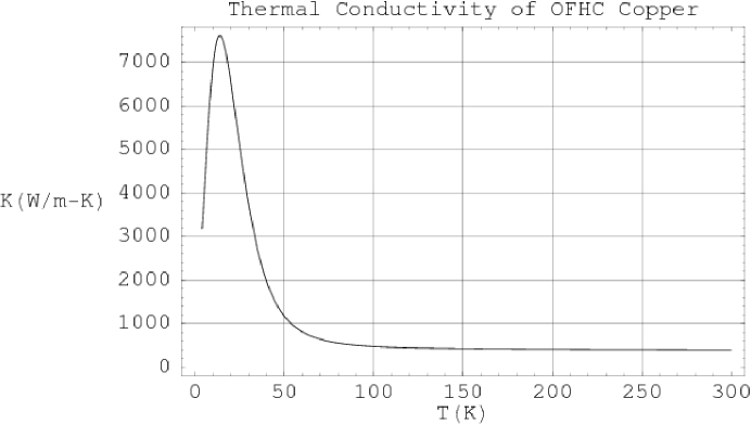
The cold head of the refrigerator interfaces with the two stages using copper strapping. Copper was chosen for its high thermal conductivity (see Fig. 12). For the coldest stage, it was necessary to machine and hard solder (using silver solder) a piece that ensured good thermal coupling on each end without mechanically stressing the refrigerator as the system is warmed and cooled (labeled #4 in Fig. 10). The thermal link from the second stage of the refrigerator cold head to the cold plate is made by four thin copper shims, each of which has a small kink (zig-zag) that helps provide strain relief. The thermal power $P$ conducted across a thermal link between temperatures $T_{1}$ and $T_{2}$ can be calculated,

$$P=\frac{A}{L}\int_{T_{1}}^{T_{2}}\!\kappa(T)dT$$ (4)

where $\kappa$ is the thermal conductivity in ${\rm(Wm^{-1}K^{-1})}$.

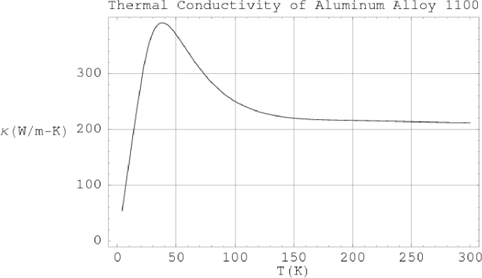
Indium film (0.01$\arcsec$ thick) provides a soft, conductive layer between the nickel-plated copper refrigerator head and the copper strapping. Indium is also used in the interface between the strapping and the cold plate. The four oxygen-free high-purity (OFHC) copper shims that conduct heat from the cold plate to the second stage of the refrigerator head are each 0.05$\arcsec$ thick, 2$\arcsec$ wide, and about 2$\arcsec$ long, yielding an area-to-length ratio $A/L=4\times 0.05\arcsec\simeq 0.005~{}{\rm m}$ (see Eq. 4). At 12 K, OFHC copper has a high thermal conductivity of $\sim 7500~{}{\rm(Wm^{-1}K^{-1})}$, so a load of 1 W produces a temperature differential of only $\sim 0.03~{}{\rm K}$ along the length of the strapping to the cold plate. The measured differential across this copper strapping agreed with this calculation to within the resolution of the Lakeshore temperature sensors we used. Aluminum alloy 1100, the common alloy of which the receiver parts are machined – including the cold plate where the sensitive receiver electronics are mounted – has a far lower conductivity at low temperatures than copper (aluminum alloy 1100 has a conductivity $\kappa\approx 10-100~{}{\rm(Wm^{-1}K^{-1})}$; see Woodcraft (2005); NIST (2008) and Fig. 13). Even with a thickness of 0.25$\arcsec$, the aluminum cold plate exhibits a $\sim 3~{}\rm K$ thermal differential. Braided copper strapping was therefore used to link the most sensitive components – the 30-GHz HEMT and two 90-GHz MMIC HEMT blocks – directly to the refrigerator head.

Figure 12: Thermal conductivity of OFHC Copper, computed from tables available on the NIST website (NIST 2008). These values have been measured in the temperature range $T=4-300~{}\rm K$.

Figure 13: Thermal conductivity of Aluminum Alloy 1100, computed from tables available on the NIST website (NIST 2008). These values have been measured in the temperature range $T=4-300~{}\rm K$.

Figure 14: Thermal conductivity of G-10, computed from tables available on the NIST website (NIST 2008). These values have been measured in the temperature range $T=4-300~{}\rm K$.

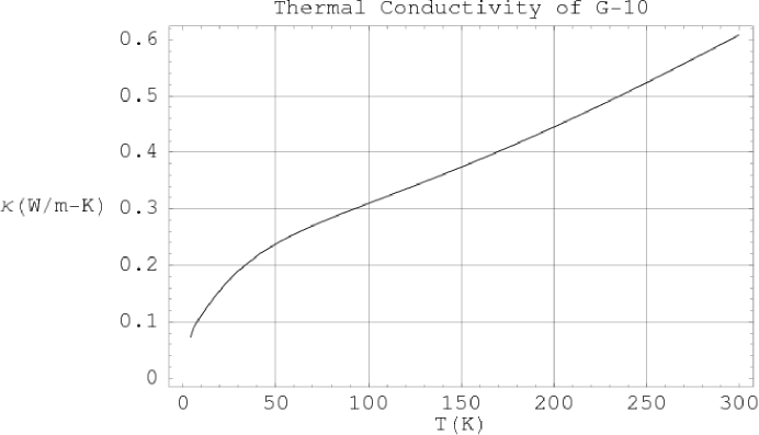
The stages of the cryostat are separated by stand-offs made of a machinable fiberglass/epoxy composite known as “G-10” or “garolite.” It has a thermal conductivity $\sim$ 0.1–0.2 ${\rm(Wm^{-1}K^{-1})}$ at temperatures from 10–100 K, and $\sim 0.6~{}{\rm(Wm^{-1}K^{-1})}$ at room temperature, making it a good insulator (see Fig. 14). The six stand-offs for the radiation shield, each 0.813 in (2.06 cm) long and with a cross-section of 0.062 in² (0.40 cm²), contribute about 0.8 W to the total thermal load on the radiation shield. Five stand-offs are used to separate the cold plate from the radiation shield. These stand-offs are each 0.5 in (1.25 cm) long and have the same cross-sectional area as the first set of stand-offs; they contribute roughly 50 mW to the cold plate.

A multi-layered blanket of aluminized mylar fills the space between the inner wall of the cryostat outer case (which is, of course, $\sim$ 300 K) and the radiation shield (see Fig. 10). The radiation shield equilibrates at $\sim$ 80 K, even though the first stage of the refrigerator is at $\sim$ 55 K, due to the poor conductivity of the aluminum of which the shield is made. This blanket reduces thermal loading due to emission, as each layer is highly reflective and will equilibrate to some temperature between 90-300 K. Thermal emission can be computed using the Stefan-Boltzmann Law ($P=b\sigma T^{4}A$), where $b$ is the emissivity coefficient of the material ($b\approx 0.10$ for aluminum), $\sigma$ is the Stefan-Boltzmann constant, $T$ is temperature (in K), and $A$ is the area of the absorbing/emitting surface. The strong temperature dependence encapsulated in the Stefan-Boltzmann Law implies that the innermost blanketing layer, which equilibrates at $\sim$ 80 K, radiates $\sim$ 200 times less than the 300 K cryostat inner wall.

In Fig. 7, the item labeled #19 is called a “getter.” The getter contains activated charcoal, which acts as a trap for contaminants in the cryostat. The charcoal, which is cold, provides a large surface area onto which contaminants are adsorbed. Note that the final receiver configuration had the getter mounted to the cold plate.

Zotefoam was chosen as the material out of which to build the receiver windows, as it also can hold vacuum (in addition to the properties discussed in the previous section). However, zotefoam is very elastic, and a window made of zotefoam alone bows under vacuum enough to be compressed against the corrugated feed horns. Since these feed horns couple directly via waveguide to the HEMT amplifiers, and are mounted on the electronics plate, they are ideally kept at the same temperature as the amplifiers. Even given the poor conductivity of zotefoam, this strong contact between it and the feed horns is enough to dominate the thermal load on the cold stage.

The bowing problem was solved by introducing a layer of mylar as a backing for the zotefoam. Thin, microwave transparent mylar, like that in the receiver windows, is strong enough to support the zotefoam, but is not robust to sharp impacts. The zotefoam layer acts as a mechanical protection for the mylar, and makes the vacuum seal.

Figure 15: The window holder, as seen looking at the bed where the window is epoxied.

Figure 16: Cross-section of the window holder, depicting where the first layer of epoxy is applied.

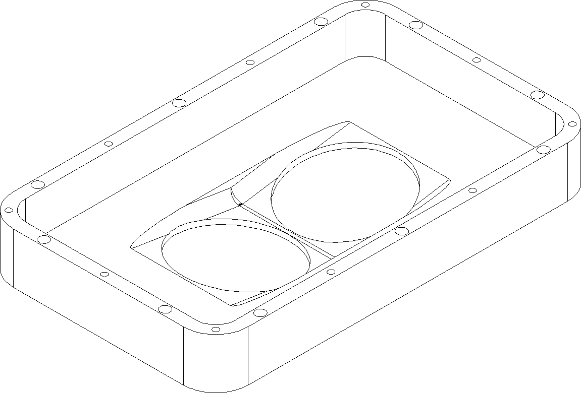
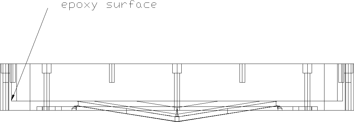
The windows are held by a custom-designed piece machined from a solid aluminum block (see Fig. 15). Two holes, each about 1.2 times larger than the outer diameter of the feed horns, allow the signal to enter. The bed of the holder provides a large, flat surface which was sandblasted to further increase the surface area. This surface was coated with a thin layer of epoxy (specifically, a clear Emerson & Cuming Eccobond^® 24, two-part epoxy with high viscosity, which avoids getting epoxy in unwanted places), and a single layer of mylar is joined here, carefully removing bubbles by hand from the interface (see Fig. 16 for an illustration of this interface). After the first layer sets, the zotefoam is joined here by applying another layer of epoxy directly above the first layer. This is done to avoid having epoxy in the optical path. After this layer of epoxy sets, one last layer of epoxy is used to fill in the $\sim$ 1/10^th inch gap around the zotefoam’s edge, and a protective plate with a large elliptical gap for the signal is mounted on the front. The final step in this process is to add a pinhole in the mylar (on the vacuum side), allowing any air/moisture to escape from between the mylar/zotefoam interface when vacuum is drawn. The final product is a zotefoam window that bows gently into the mylar without making contact with any of the components inside the cryostat.

4 Back-end Electronics

Figure 17: Photo of Ebox (lid removed), set up for 30-GHz observations. The Ebox houses the modules used to control and process signals from the receiver. See text in §1 for a description of the electronics. Note that the bias-tuned Gunn (BTG), the module to control the bias-tuned Gunn (the “BTG Mod” in Fig. 18), and the IF switch had not been installed at the time of this photo, as they were only required for 90 GHz observations. They were later installed in locations 12 and 20, respectively. The fiber bundle and power cables enter the Ebox at location 16. The refrigerator head (13) for the receiver (located behind the Ebox), the receiver enclosure’s chiller line (14), the chiller heat exchanger (15), and the TEC cooling fans (17) can all be seen above and outside the Ebox. The internal Ebox air circulation fans at label 18. A spring that assists in lifting the Ebox is labeled 19. The walls of the Ebox are lined with an open-cell PVC foam for insulation, which was painted white to prevent degradation and flaking due to weathering.

Figure 18: Layout of Modules in the Ebox. Connectors are shown in green.

1 Overview of the back-end electronics

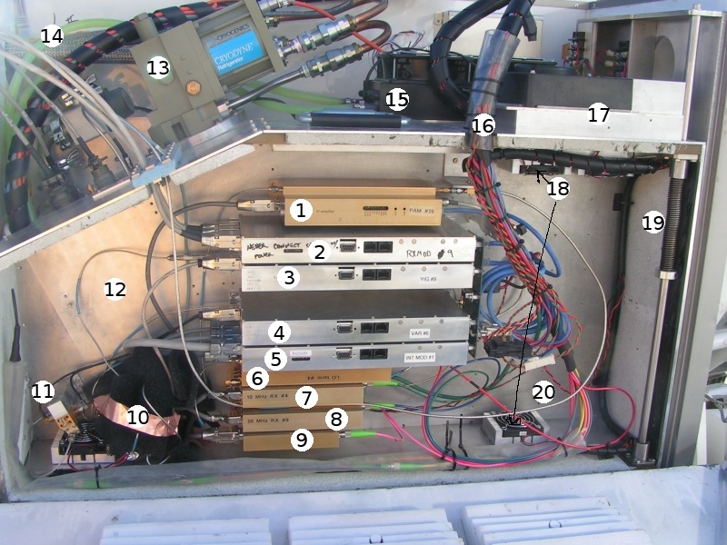
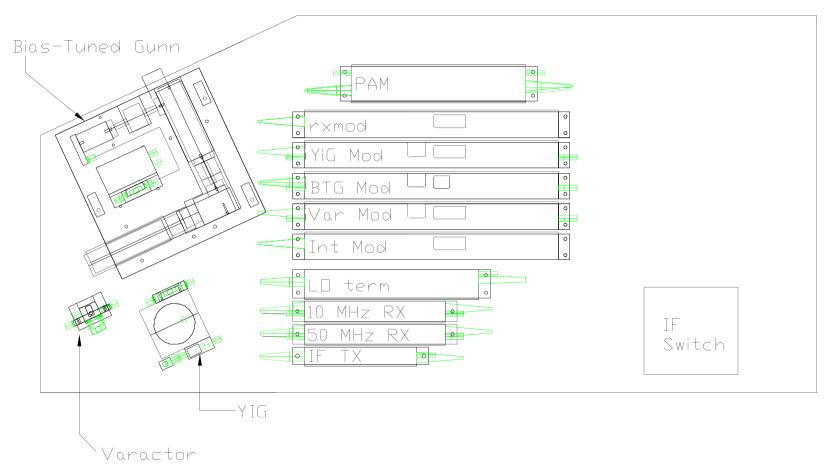
All support electronics for the receiver are located in a large, thermally-regulated, insulated box, called the “Ebox” (see Fig. 17). The Ebox is placed within the receiver enclosure, just outside the cryostat. The primary components in this box (shown schematically in Fig. 18) are:

• An IF switch, used to select the receiver output appropriate for 30 or 90-GHz observations. The IF switch is mounted in location #20 in Fig. 17.

• A pre-amplifier module (PAM in Fig. 18, #1 in Fig. 17), which is primarily an IF amplifier, is common to both receivers as it follows the IF switch. The PAM also includes a set of precisely-calibrated attenuators (in 0.5 dB steps, up to a total attenuation of -30 dB), both on the input and output of the module. These attenuators are useful in avoiding compression effects when the power becomes high enough to saturate electronics further down the signal chain. Since the hot load calibrator (a thermal blackbody at ambient temperature) increases the receiver output power by a factor $\sim(300~{}{\rm K})/T_{\rm sys}\sim 4-6$, where $T_{\rm sys}\sim$ 40–50 K, these attenuators are also inserted during calibrations to prevent compression of the signal (for more information, see §3).

• A power supply for the receiver (labeled “rxmod” in Fig. 18 #2 in Fig. 17). This powers both the 30 and 90-GHz receivers.

• An high-frequency oscillator, based on a Yttrium Indium Gallium (YIG in Fig. 18, #10 in Fig. 17) diode in a cavity, that operates at 8.972 GHz. The module that monitors the YIG’s status is labeled #3.

• The varactor, a “variable capacitance” component (#11 in Fig. 17) that is used to produce harmonics of the YIG frequency as well as lock the phase of the LO. A phase-lock loop (PLL), controlled by electronics in the correlator trailer, locks the phases of all antennae to a single reference. The module that controls the varactor is #3.

• A bias-tuned Gunn (BTG) oscillator, which is the 90-GHz system’s equivalent of the YIG. This uses a Gunn diode forced into oscillation within an adjustable waveguide cavity. This was later installed in location #12 in Fig. 17, while the module to control it was installed between #3 and #4 (“BTG Mod” in Fig. 18).

• A dielectric resonance oscillator (DRO), which supplies the fixed 17.5 GHz secondary LO used by the 90-GHz system’s secondary mixer. This is mounted on the same plate as the BTG, so it was also installed in location #12 in Fig. 17.

• Various CANBUS (a protocol like TCP/IP that allows daisy-chaining) controlled electronics, used to control the various oscillators and reference frequencies of the PLL and lobe rotator (which accounts for the part of fringe tracking due to movement of the source across the sky), regulate the temperature, etc. Among these is the interface module (“Int Mod”, #5 in Fig. 17), which monitors the phase reference and lobe rotator. These references are received by the 10 and 50 MHz receivers (#7 and #8 in Fig. 17).

• The local oscillator terminator (“LO Term” in Fig. 18, #6 in Fig. 17), which locks the YIG to the ninth harmonic of a central, synthesized reference frequency with the 10 MHz signal mentioned above. This phase lock loop is separate from, but analogous to, the one which locks the varactor to the YIG using the 50 MHz reference.

• An optical IF band transmitter (called the “OTX”; labeled “IF Tx” in Fig. 18, #9 in Fig. 17), which takes as its input the output of the PAM. This sends the signal over fiber optics (#16 in Fig. 17) to the downconverter and correlator (which are discussed in §1 & 2, respectively).

2 Thermal considerations for the electronics box

Thermal stability is the primary motivation for the implementation of this insulated electronics box. The thermal sensitivity of the amplifiers, local oscillators, and fiber optics (whose lengths change with temperature) leads to phase variations during periods of poor thermal regulation. While these effects, discovered during commissioning operations, varied from antenna to antenna, one extreme example exhibited $\pm 45^{\circ}$ phase oscillations as the temperature varied sinusoidally about its nominal regulation temperature by $\pm 2.5^{\circ}$C (which could happen even with the final thermal regulation in place). Since these oscillations had periods on the order of 15-20 minutes, the same frequency as that of our calibration observations, the sampling of these phase changes is not frequent enough to remove the effects through data calibration. This problem was eventually solved with better regulation algorithms and the occasional manual intervention by the observer.

Thermal regulation of the electronics box, utilizing thermo-electric coolers (TECs, or Peltier junctions), is set up so that the temperature at a single point on the electronics mounting plate is kept within $\pm 0.125^{\circ}$C of the 32^∘C (28^∘C) set point in the summer (winter). The thermal differentials within this box are reduced by fans, and by the large thermal mass and high thermal conductivity of the 1/4-inch aluminum plate to which all the electronics are mounted. A small amount of silicone grease (heatsink compound) is used to ensure decent conductivity between the electronics modules and the mounting plate.

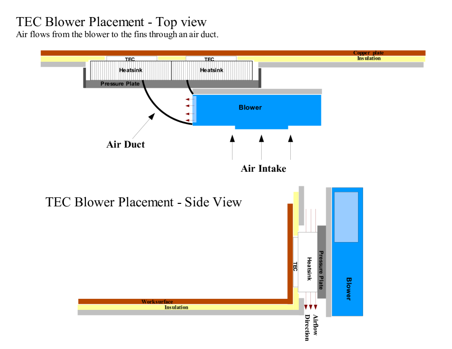
A conceptual overview of the TEC setup for the electronics box is show in Fig. 19. Ambient air is forced, by a large impeller fan (#17 in Fig. 17), through the fins of the heatsink attached to the hot side of each TEC, thereby carrying away the heat. Good thermal contact between the heatsink and the TEC is ensured by the pressure plate, which is held down by five springy Belleville washers, each providing 20-30 pounds of force. This setup also forces the cold side of the TECs onto a copper plate that makes thermal contact with the electronics mounting plate, labeled “worksurface” in Fig 19. Since the TECs are ceramic, their porous surfaces are coated with a layer of heatsink compound, which fills the pores and provides more surface area for thermal contact. Open-cell foam insulation isolates the temperature-regulated copper plate and worksurface from the warmer outside air.

Figure 19: TEC Blower Conceptual Diagram, courtesy Marshall Joy and Georgia Richardson. Ambient air from the receiver enclosure is forced through the heatsink fins by the blower (see Fig. 17, #17). These copper heatsinks are thermally coupled to the hot sides of the TECs (which are $\gtrsim 20^{\circ}\rm C$ hotter than the worksurface side). The TECs diffuse more heat away from the worksurface than toward it, thus removing heat from the Ebox.

The TECs can be operated at a maximum power of $P_{\text{max}}=300$ W (10 A at 30 V, DC), removing $P_{\text{max,remove}}=\xi P_{\text{max}}$ for TEC efficiency $\xi$. With cooling efficiencies of $\xi\approx 30\%$, they can keep a thermal load of up to 90 W regulated at a desired set temperature. The electronics within the Ebox draw $\sim$3 A at 24 V (DC), and therefore dissipate $\sim$ 72 W of heat. There is a remaining thermal load that is due to both the finite thermal conductivity of the G-10 supports and foam insulation of the Ebox, and to the imperfect thermal isolation provided by the Ebox.

The Ebox insulation is a rigid PVC foam, chosen because it is the best insulating foam offered by McMaster-Carr. The conductivity of the foam is $90~{}{\rm mW\cdot in/ft^{2}/K}$ ($0.17~{}\rm btu\cdot in/ft^{2}/^{\circ}F$). With $\sim 11~{}\rm ft^{2}$ of 0.375 in foam insulation, 2.6 W of heat flow through this insulation for each degree of differential between the outside and inside of the box (see Eq. 4), In practice the electronics box cannot maintain a temperature more than $\sim 1^{\circ}$C less than the ambient temperature of the receiver enclosure, due to leaks that allow some air exchange between the inside and outside of the box.

5 The Correlator Trailer

The signal from each telescope is sent over fiber optic cables, located in conduits underground (as illustrated in Fig. 1), to an air-conditioned trailer – referred to as the “correlator trailer” – containing the instrumentation necessary to downconvert (§1) and correlate (§2) the signals. The correlator trailer also houses the computer that controls the array and collects all data taken during an observation.

1 Downconverter

Figure 20: Block Diagram of the SZA Band Downconversion, showing how the sky observation frequencies 26.938–34.938 and 90.78–98.78 GHz are split into the sixteen digitized bands, each 500 MHz in bandwidth, that are the input to the correlator. See description in the text (§1). Bands shown in red are the side bands that are not used.

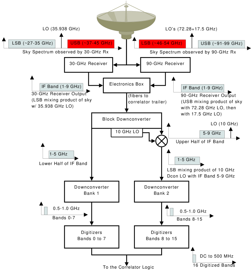
The 1–9 GHz IF is processed by an array of mixers, amplifiers, and bandpass filters, known collectively as the “downconverter,” which splits the IF into sixteen 500 MHz bands running from 0.5–1 GHz (see Fig. 20). The reason for using this range is that electronics that can handle 0.5 GHz and 1 GHz are similar, while those that could handle a signal from 0–0.5 GHz; for instance, DC signals cannot be capacitively coupled.

Here I describe the full signal downconversion chain, starting from the sky frequencies 26.938–34.938 and 90.78–98.78 GHz, and ending with the sixteen digitized 500 MHz bands that constitute the input to the correlator. Figure 20 illustrates this signal chain.

The tertiary mirror of each telescope selects either the 30 or the 90-GHz receiver. In the 30-GHz receiver system, the lower side band (LSB) mixing product of the sky with a 35.938 GHz local oscillator (LO) places sky frequencies 26.938–34.938 GHz in the 1–9 GHz IF band. In the 90-GHz receiver, a 72.28 GHz LO (in the current tuning scheme) mixes with sky frequencies 90.78–98.78 GHz, producing a 18.5–26.5 GHz upper side band (USB) product; a second LO at 17.5 GHz mixes with this to place the 90-GHz receiver output (also USB) in the 1–9 GHz IF band (see Fig. 21 for more details on the downconversion in the 90-GHz receiver). Note that the 30-GHz receivers have a full bandwidth of 10 GHz, while the 90-GHz receivers have a much broader bandwidth that allows observations from 85–115 GHz. For both systems, the back-end electronics determine what range of sky frequencies are observed.

Figure 21: Detailed Diagram of the 90-GHz Receiver Downconversion, showing how the sky observation frequencies are brought down to the 1–9 GHz IF band (see Fig. 8 for details on the receiver RF components). This figure accompanies the broader downconversion scheme illustrated in Fig. 20. In the current tuning scheme, sky frequencies 90.78–98.78 GHz are mixed ($\otimes$) with a 72.28 GHz LO (the bias-tuned Gunn), producing an 18.5–26.5 GHz USB product. Sky frequencies $<85~{}\rm GHz$ are blocked by the high pass filter, so no LSB mixing product is produced (e.g. the band shown in red). The bandpass filter passes the 18.5–26.5 GHz USB product to a second mixer. The second LO, at 17.5 GHz, mixes with this 18.5–26.5 GHz USB product to place the 90-GHz receiver output in the 1–9 GHz IF band. This 1–9 GHz IF signal is the input to the back-end electronics common to both the 30 and 90-GHz systems. See §1 for more details.

Band IF Band Range 30-GHz Sky Frequencies 90-GHz Sky Frequencies (#) (GHz) (GHz) (GHz) 0 1.0–1.5 34.688 91.030 1 1.5–2.0 34.188 91.530 2 2.0–2.5 33.688 92.030 3 2.5–3.0 33.188 92.530 4 3.0–3.5 32.688 93.030 5 3.5–4.0 32.188 93.530 6 4.0–4.5 31.688 94.030 7 4.5–5.0 31.188 94.530 8 5.0–5.5 30.688 95.030 9 5.5–6.0 30.188 95.530 10 6.0–6.5 29.688 96.030 11 6.5–7.0 29.188 96.530 12 7.0–7.5 28.688 97.030 13 7.5–8.0 28.188 97.530 14 8.0–8.5 27.688 98.030 15 8.5–9.0 27.188 98.530

Table 1: The 1–9 GHz IF band is separated into 16 bands, as outlined in Fig. 20. These are the central sky frequencies of both the 30 and 90-GHz SZA systems that correspond to the downconverted IF bands, discussed in §1. Note that higher band number corresponds to a lower sky frequency for the 30-GHz system because it uses the lower side band.

Back-end electronics in the electronics box select the proper receiver output and send the signal over fibers to the correlator trailer (see Fig. 1). The IF is then split into 1–5 and 5–9 GHz bands by the block downconverter. The lower half of the IF, from 1–5 GHz, is passed directly to the second stage downconverter. The 5–9 GHz band is mixed with a 10 GHz LO, also in the block downconverter, and the LSB mixing product (from 1–5 GHz) continues to the second stage downconverter. I use the $\otimes$ symbol to represent the mixer, which is located within the block downconverter, to clearly denote how the 1–9 GHz IF band is first split into 1–5 and 5–9 GHz.

The second stage downconverters mix and filter each 1–5 GHz band into sixteen separate 0.5–1.0 GHz bands, listed in Table 1. Each 0.5–1.0 GHz band is then digitized at a sampling frequency $f_{s}=1$ GHz. This sampling operation digitally aliases each 0.5–1.0 GHz band to a 0–500 MHz baseband, digitized signal. This sampled signal is the input to the SZA correlator, discussed in the next section.

2 The SZA Correlator

In the discussion of interferometry presented in §3, details about the process of interfering the signals from a pair of antennae, and the instrument that performs this cross-correlation, were for simplicity ignored. I now discuss the correlator, which is the single instrument most crucial for performing interferometry. Fig. 22 shows a photo of the SZA correlator.

The cross-correlation $r_{xy}(m)$ for digital time delay $m$ of two discrete-time signals $x(n)$ and $y(m+n)$ (delayed by $m$ samples with respect to $x(n)$), such as the digitized signals from a pair of antennae, is defined

$$r_{xy}(m)\equiv\sum_{n=-\infty}^{\infty}x[n]~{}y[m+n].$$ (5)

Here, $n$ is a sample taken at time $t=n\tau$ for sampling period $\tau\equiv 1/f_{s}$, and $m$ a whole number lag – a discrete time delay – applied to one antenna’s signal. Since the SZA bands are sampled at $f_{s}=1$ GHz, $\tau=1$ ns. In a real instrument, we cannot sum over the infinite number of samples indicated in Eq. 5. For the SZA, correlation is performed for 32 lags of each signal, after having been properly delayed by fringe tracking and downconverted to 0.5–1 GHz bands (as discussed in § 1). The overall effect of the correlator is to multiply the signals from two antennae, sliding one signal past the other. Since the signals $x(n)$ and $y(n)$ scale as voltage, the correlator output scales as voltage-squared; cross-correlation is therefore proportional to the power received by an antenna.

Figure 22: Photo of the SZA Correlator and Downconverter, courtesy David Hawkins.

We are accustomed to dealing with visibilities as a function of frequency. Visibilities, when calibrated against an astronomical source of known flux, give the flux at each data point in u,v-space, for each frequency in a spectrum (see §3). The spectrum is simply obtained by Fourier transforming the correlated data.

The SZA correlator is an XF or lag-correlator, where X stands for the cross-correlation, and F stands for the Fast Fourier Transform (FFT). The SZA correlator performs cross-correlation in the time domain, but note that FX correlators are also common, since correlation has a simple Fourier relation

$$r_{xy}(m)=\mathcal{F}\{X[k]^{*}Y[k]\},$$ (6)

where $X[k]$ and $Y[k]$ are the Fourier transforms of $x(n)$ and $y(n+m)$ for discrete frequencies $k$, $\mathcal{F}$ is the Fourier transform operation, and ^∗ denotes the complex conjugate.

The FFT is a computationally efficient implementation of the Discrete Fourier Transform (DFT), which in turn is a truncation of the Discrete Time Fourier Transform (DTFT). The DTFT is mathematically complete (e.g. it satisfies Parseval’s Theorem; see Oppenheim et al. 1999; Bracewell 2000, for further information), and becomes the familiar (continuous time) Fourier Transform in the limit of infinitesimally small steps in time.

The DTFT is:

$$X(\omega)=\sum_{\scriptscriptstyle n=-\infty}^{\scriptscriptstyle\infty}x(n)~{}e^{\scriptscriptstyle-j\omega n}$$ (7)

where

$$x(n)=(1/2\pi)~{}\int_{\scriptscriptstyle-\pi}^{\scriptscriptstyle\pi}X(\omega)~{}e^{\scriptscriptstyle j\omega n}d\omega.$$ (8)

The DFT is a special case of the DTFT, where the number of samples is limited to a finite number $N$. This has the effect of discreting frequency at $\omega=2\pi k/N$, where $k=N(f/f_{s})$ is the discretized wavenumber. In the DTFT, $X(\omega)$ wraps outside the range $\omega=[-\pi,\pi]$; in the DFT, $X(\omega)$ is sampled at only the discrete values of $k$, and $X(k)$ wraps outside the range $k=[0,N-1]$. The DFT is:

$$X(k)=\sum_{\scriptscriptstyle n=0}^{\scriptscriptstyle N-1}x(n)~{}e^{\scriptscriptstyle-j2\pi kn/N}$$ (9)

where

$$x(n)=(1/N)~{}\sum_{\scriptscriptstyle k=0}^{\scriptscriptstyle N-1}X(k)~{}e^{\scriptscriptstyle j2\pi kn/N}$$ (10)

The substitutions that take us from the DTFT to the DFT have the effect of limiting the frequency resolution to $N/2$ elements (in the Nyquist bandwidth of $f_{s}/2$; there are $N$ discrete $k$’s in the range $f=[-f_{s}/2,f_{s}/2]$). Notice that the wrapping in the DTFT and DFT (Eqs. 8 & 10) is the same as wrapping every $f_{s}$ in frequency, or every harmonic of the sampling frequency; this aliasing is simply that due to Nyquist sampling at $f_{s}$, mentioned in §1. Only the range $k=[0,N/2-1]$, corresponding to frequencies $\omega=[0,\pi]$, contains unique spectral information. Since the time-domain signal is real, its transform is Hermitian, meaning those frequencies above $f_{s}/2$ are the complex conjugate of the positive frequencies. Table 2 lists the 17 channels produced by FFT-ing the 32 samples.

Channel Frequency (#) (MHz) 0   0.00 1  31.25 2  62.50 3  93.75 4 125.00 5 156.25 6 187.50 7 218.75 8 250.00 Channel Frequency (#) (MHz) cont’d cont’d 9 281.25 10 312.50 11 343.75 12 375.00 13 406.25 14 437.50 15 468.75 16 500.00

Table 2: Each 500 MHz band has 17 channels, numbered 0–16. Channels 0 and 16 are both attenuated by the 500 MHz bandpass filters used in the downconverter §1, and are not used for data. Note that these are discrete frequencies that arise from the DFT of a discrete-time signal (Eqs. 9), rather than continuous bands.

In the time domain, the limited number of correlator lags $m$ used in the DFT is equivalent to rectangular windowing – the one-dimensional equivalent to the top hat function – of the correlated signal $r_{xy}(m)$ (Eq. 5). Outside of the range $n=[0,N-1]$ (in discrete time), the signal is zero, and this has important implications when interpreting the DFT as a power spectrum (which are discussed in §3).

The mathematics of the cross-correlation and Fast Fourier Transform (FFT) are programmed into field-programmable gate arrays (FPGAs), which can be faster than using general-purpose processors to perform digital correlation. The raw visibilities produced by this process are averaged for 0.5 second intervals and stored to disk as raw visibilities in correlator units. The reader is encouraged to see Hawkins et al. (2004) for further details, where the SZA correlator is described in much greater detail.

3 Thermal Considerations for the correlator trailer

The correlator trailer draws $\sim 1$ MW of power, and thus requires an industrial-strength air conditioner (A/C) with two independent compressor units (though much of this power is drawn by the A/C itself, and its heat is dissipated outside). At the beginning of SZA commissioning, we used a state-of-the-art air conditioner with a commercially-available governor that can keep the temperature within $\pm 1^{\circ}$C of a desired set point. It was soon discovered, due to the temperature sensitivity of the digitizers, that the 20 minute air conditioner cycling of $\pm 0.25^{\circ}$C led to $\pm 3^{\circ}$ phase variations in the data (see Fig. 23), and a more robust solution had to be found.

Figure 23: Plot of phases on a single baseline (Baseline 0-1) and the corresponding downconverter temperatures during the same period. The blue lines are the temperatures measured in the downconverters for Antennae 0 (dashed line) and 1 (solid line). The black line is the phase of the raw data on baseline 0-1, taken while staring at a strong point source, which ideally has flat, constant phase (see §2 for details). Note that thermal variations in adjacent digitizers, due to cycling of the A/C, of 0.5^∘C (peak to peak) produced 6^∘ phase variations. Modifications to the A/C removed these thermal oscillations on short time scales (see Fig 24).

Figure 24: Plot of phases on a single baseline (Baseline 0-1) and the corresponding downconverter temperatures during the same period. The blue lines are the temperatures measured in the downconverters for Antennae 0 (dashed line) and 1 (solid line). The black line is the phase of the raw, uncalibrated data on baseline 0-1, taken while staring at a strong point source, with the linear slope and mean value removed. Note that this is on a much shorted time scale than that of Fig. 23, but is long enough to have shown 3 full cycles of the A/C if they had persisted. Any residual phase error is both negligble and is removed by calibration (see §3)

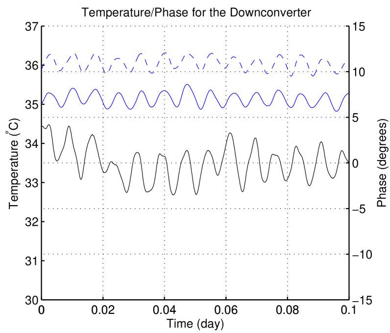
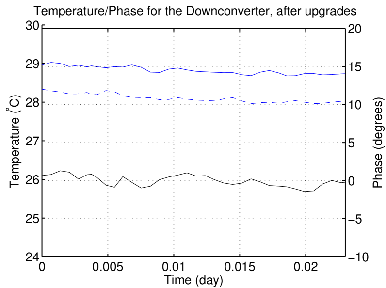
The resolution to this problem was largely worked out by the SZA engineer, Ben Reddall. He removed the governor and set the A/C to be continuously on. He then modified the unit so that louvers could push the air through the heat exchanger of one compressor at a time, so that the other compressor could be shut off when not necessary. This strong, continuous air flow in a closed cycle ensures good mixing and stability within the trailer; it also prevents the active compressor from icing up, as it essentially doubles the airflow through it. Various layers of insulation further contributed to the thermal stability of the trailer. The final steps implemented by Ben Reddall were the addition of water bottles (water has a high thermal capacity) to the air supply duct, and of three 1 kW space heaters used during the winter. The heaters help prevent the A/C, which must be run continuously, from freezing on cold winter nights. Figure 24 demonstrates the continuing success of the correlator trailer thermal solution, three years after it was implemented.

The temperature in the correlator trailer typically varies by 20^∘C over the day, but does so in a way that these slow, diurnal phase changes are common mode to the fibers and electronics. The slowly-changing phase drifts produced by these temperature changes can be tracked using our standard astronomical calibration (see §3) and removed from the data.

Chapter 2 Sources of Contamination

This chapter addresses two sources of contamination found during the SZA commissioning phase: radio interference from external sources and antenna cross-talk. While I have attempted to make this palatable for those who are not engineers or radio astronomers, the information is best suited to an audience interested in building and debugging a radio interferometer.

1 Radio Interference

Here we consider the problem of radio frequency interference (RFI), which we found in our early observations to be contaminating frequency channels or even entire bands. A “birdie,” the colloquial name for RFI, is in general some contaminating, non-astronomical signal, which can increase the scatter in the radio visibilities at the birdie frequency, corrupting data in a given channel or even a whole band (discussed in §3). The strongest birdies are generally from sources local to the antenna electronics, and could be the mixing product of the local oscillator (LO), the LO reference, and/or the YIG. Birdies can also come from external transmissions, generally ground-based sources (e.g. military communications or satellite uplinks) or geostationary satellites.

In this section, we examine ways of lessening the impact of birdies, since they could potentially contaminate maps made from observations with the SZA. For simplicity, we consider a birdie to be an ideal sinusoidal signal. We calculate how much fringe tracking helps to reduce birdies, since they are stationary with respect to the antennae and lose coherence in the cross-correlated data.

Early observations with the SZA revealed the presence of a strong birdie, just outside our IF band, at the receiver output frequency 9.022 GHz. This birdie arose in the output of the receivers as the mixing product of the YIG 3${}^{\text{rd}}$ harmonic ($3\times 8.972~{}\rm{GHz}=26.916~{}\rm{GHz}$) and the 35.938 GHz LO ($35.938~{}\rm{GHz}-26.916~{}\rm{GHz}=9.022~{}\rm{GHz}$). The 30-GHz receivers detected both the YIG 3${}^{\text{rd}}$ harmonic emitted within their own Eboxes and those from adjacent antennae (§3 for information on the YIG oscillator). This birdie showed up in Band 15, which is the lowest sky frequency band (26.938–27.438 GHz), despite the fact that this band runs from 8.5–9 GHz, and the birdie was 9.022 GHz.

We demonstrate in this section that an additional 23 dB of attenuation, at the birdie’s source, was required to bring the birdie to less than 10% of the rms noise level via fringe tracking. We then proceed to consider how a birdie can corrupt all the channels in a band, even if the birdie is a pure tone, singular in frequency. Finally, we demonstrate that a clever retuning of local oscillators can avoid band corruption by insuring all the birdie’s power appears in one channel, which can readily be flagged and excised from the data.

1 The Effect of Fringe Tracking

Since birdies come from sources not associated with the field being observed, they can be treated as an untracked source. Since the SZA birdie was local to the antenna, it was effectivley moving across the sky in the opposite direction as the astronomical source being observed. The instantaneous correlations of the birdie signal affecting a pair of antennae do not sum up coherently over time (see §3), and the birdie is therefore attenuated by this loss of coherence. The factor by which the birdie is attenuated, $F_{b}$, can be calculated as a sinc function of the fringe frequency $\nu_{f}$ (the rate at which an untracked source moves across the sky) and the integration time $\tau_{a}$. The attenuation factor is

$$F_{b}=\frac{\sin(\pi\nu_{f}\tau_{a})}{\pi\nu_{f}\tau_{a}},$$ (1)

where $\nu_{f}$ is the fringe frequency

$$\nu_{f}=u~{}\!\omega_{\scriptscriptstyle e}\cos(\delta),$$ (2)

$\omega_{\scriptscriptstyle e}$ is the earth’s angular velocity, ($\omega_{\scriptscriptstyle e}=7.29115\times 10^{-5}~{}\text{rad s}^{-1}$), $\delta$ is the source’s declination, and $u$ is the Fourier conjugate (in u,v-space, the standard notation used by radio astronomers) of the baseline along the east-west direction, normalized by the wavelength of observation:

$$u=X_{\scriptscriptstyle\lambda}\sin H+Y_{\scriptscriptstyle\lambda}\cos H.$$ (3)

Here $H$ is the hour angle of the source, where $H=0^{h}$ corresponds to the meridian, and each hour increment is 15^∘. $X_{\lambda}$ and $Y_{\lambda}$ are respectively the x (north-south) and y (east-west) components of the baselines divided by the wavelength at which the observation is made. A longer baseline increases the fringe frequency, since it yields a tighter, more highly-resolved fringe pattern on the sky. A source at $\delta=0^{\circ}$ (in the equatorial plane) moves most quickly across the sky, so the fringe frequency $\nu_{f}$ is highest there. A point source at the pole, on the other hand, would not move through fringes at all.

The $1/{\pi\nu_{f}\tau_{a}}$ envelope of the birdie attenuation factor (denominator of Eq. 1) results from the time averaging of the measured visibities, the smallest binning of which is a 1/2 second frame (see §2). We are interested in how much the birdie is attenuated during an observation, and how this compares to the Gaussian noise floor of the same observation. The noise floor decreases according to (see, e.g. Rohlfs & Wilson 1996; Thompson et al. 2001):

$$\frac{\Delta T_{A}}{T_{\rm sys}}=\frac{M}{\sqrt{\Delta\nu\times\tau_{a}}}.$$ (4)

In the above equation, $M$ is a factor – less than or equal to unity – that accounts for the quantization noise in the correlator system, $\tau_{a}$ is the integration time, $\Delta\nu$ is the bandwidth, and $T_{A}$ is the antenna temperature.

2 Can Fringe Tracking Beat Down the Birdie?

We consider here if the SZA 9.022 GHz (IF band) birdie that plagued Band 15 of the SZA 30-GHz system (see Table 1) in the first few months of operation could be sufficiently attenuated by fringe tracking. We assume our source is at declination $\delta=0^{\circ}$, which is our best case scenario; this yields the highest fringe frequency, since the source moves most rapidly across the sky. If our source were at the north celestial pole, on the other hand, fringe tracking would not attenuate the birdie at all. Clearly, we cannot rely in all cases on fringe tracking to eliminate birdies. We will also for simplicity assume our source is close to the meridian (i.e. near transit). With $H\simeq 0$, the $X_{\lambda}$ component is negligible (see Eq. 3), simplifying the calculation.

Let us set $Y_{\lambda}=1000$ (see Eq. 3). For the SZA, this would be among the longest of the inner array baselines, with a 10 meter, east-west baseline component while observing at 30 GHz. If we chose a purely north-south baseline ($Y_{\lambda}=0$), a source near transit would give $u=0$, and fringe tracking would not attenuate the birdie at all (see Eq. 2). Again, this indicates that fringe tracking is not a panacea for reducing birdies, but we proceed to compute how much it helps in our best case scenario for the inner array.

Calculating the fringe frequency (Eq. 1) for these conditions, $\nu_{f}\simeq 7.3\times 10^{-2}\rm~{}Hz$. We can see that $F_{b}$ hits its first null at $\tau_{a}=1/\nu_{f}\simeq 14\rm~{}sec$, and we might be tempted to choose this as our integration time so that no stationary sources could affect us. Since this frequency is different for each baseline, it is clear that this scheme will not work.

We can proceed in calculating the birdie’s attenuation without needing to know $M$ and $T_{\rm sys}$ (in Eq. 4) by measuring the ratio of the birdie signal power with fringe-tracking off (which is therefore unattenuated by integration) to the noise level in a known time interval. Given the functional behavior of the birdie’s attenuation (Eq. 1) we only measure the birdie’s unattenuated amplitude $A_{b,0}$ and the noise’s rms amplitude $A_{n}(\tau_{m})$ in a given time interval $\tau_{m}$, with fringe tracking off. It should be noted that the noise integrates down as $1/\sqrt{\tau}$ (as in Eq. 4) without regard to fringe tracking, so it is reasonable to compare the noise levels for given integration times, regardless of whether fringe tracking is on. The birdie and fringe amplitudes as functions of time are given by:

$$A_{b}(\tau_{a})=A_{b,0}~{}F_{b}(\tau_{a})$$ (5)

and

$$A_{n}(\tau_{a})\sqrt{\tau_{a}}=A_{n}(\tau_{m})\sqrt{\tau_{m}}$$ (6)

so that the ratio of the birdie to the noise level for integration time $\tau_{a}$ is:

$$\frac{A_{b}(\tau_{a})}{A_{n}(\tau_{a})}=\frac{A_{b,0}~{}F_{b}(\tau_{a})}{A_{n}(\tau_{m})\sqrt{\tau_{m}/\tau_{a}}}$$ (7)

With fringe tracking off, the level of the 9.022 GHz birdie was measured to be $\sim 250$ times the noise in a 20 second, uncontaminated integration. Since it’s more convenient to express integration times in seconds, we solve for $A_{b,0}$ normalized to the noise in a 1 s integration:

$$A_{b,0}=250~{}A_{n}(20~{}\rm s)=\frac{250}{\sqrt{20}}A_{n}(1~{}\rm s).$$ (8)

Plugging the ratio $A_{b,0}/A_{n}(1~{}\rm s)$ into Eq. 7, we find the ratio of the birdie to the noise level after time $\tau_{a}$ (in seconds):

$$\frac{A_{b}(\tau_{a})}{A_{n}(\tau_{a})}=\frac{250}{\sqrt{20}}~{}\!F_{b}(\tau_{a})\sqrt{\tau_{a}}$$ (9)

Taking the local maxima of $F_{b}$ (defined in Eq. 1) as our worst case scenario for the birdie’s amplitude, we ignore the sinusoidal component of the sinc function and keep the $1/(\pi\nu_{f}\tau_{a})$ envelope. This yields:

$$\frac{A_{b}(\tau_{a})}{A_{n}(\tau_{a})}=\frac{250}{\sqrt{20}}\,\frac{1}{\pi\nu_{f}\sqrt{\tau_{a}}}=\frac{17.8}{\nu_{f}\sqrt{\tau_{a}}}.$$ (10)

Now, we can solve for the time when the envelope for the birdie amplitude falls below the noise floor. For our fringe rate $\nu_{f}$, we find that it takes about 16.5 hours for this birdie to integrate down to the same level as the noise. This of course violates the assumption that the source is near transit. Furthermore, this time scale is much longer than any amount of time we would sensibly bin as a single data point.

We would like the birdie to be attenuated to $<10\%$ of the noise level in each binned data point, so that maps are relatively unaffected by the birdie (with a $\sim$ 5-$\sigma$ cluster detection, the birdie would affect the SZE flux on the $2\%$ level, which is less than our calibration uncertainty). To get this birdie down to the 10% level in a 5 minute integration, the maximum time which we might reasonably bin into a single data point, we need about 22 dB of attenuation on each antenna. When observing sources at higher declinations, additional attenuation would be required to compensate for the lower fringe frequency $\nu_{f}$. A source at $\delta=37^{\circ}$ takes 25% longer to beat the birdie down to the noise level of a $\delta=0^{\circ}$, since its fringe frequency is 80% of the $\delta=0^{\circ}$ value. Conversely, an extra dB of attenuation would be required to bring the birdie down to the same level in the same time. Therefore, we would need 23 dB of attenuation of the birdies at their sources in order for this measured birdie not to affect a typical SZA observation.

In Eq. 10, we ignored the fact that $F_{b}$ varies sinusoidally (as in Eq. 1). In a typical SZA observation, many integrations are taken, and are often binned into intervals ranging from 20–300 s. For each binned data point, the birdie level would vary randomly (since $\nu_{f}$ changes throughout the observation), with both positive and negative variations that are several times larger than the noise (e.g. 250 times larger for a 20 s observation, as measured before attenuation). Thus, as long as the fringe rate $\nu_{f}\neq 0$ a birdie would increase the scatter in the data taken at that frequency, rather than integrating to a coherent signal.

3 Spectral Leakage

As noted in §2, the limited number of samples used in correlation has the effect of rectangular windowing of the cross-correlated data. In this section we examine how a sinusoidal signal – such as an idealized birdie – can contaminate an entire band of data, rather than only appearing at its frequency. This phenomenon is called “spectral leakage.”

Figure 1: The rectangular window function and its transform. Left: The rectangular window function $w(n)$ in the time domain. Right: Magnitude of the Fourier transform of $w(n)$, $|W(k)|$. $w(n)$ is unity for $n=[0,31]$, corresponding to 32 discrete samples in time (i.e. the digitized waveform), and zero outside this range. $|W(k)|$ is unity for $k=16$ and $k=-15$, and zero at all other integer values of $k$. See discussion in text.

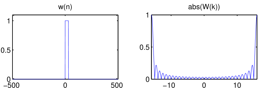
Consider a birdie at frequency $f_{0}=k_{0}f_{s}/N$, where the signal is sampled $N$ discrete times at a sampling frequency $f_{s}$, and $k_{0}$ is the birdie’s wavenumber. Let $x(n)$ be the discrete-time representation of the continuous, sinusoidal birdie signal (i.e. the digitally-sampled birdie, cross-correlated with a similar birdie from another antenna, idealized to a sine wave).

$$x(n)=A\sin\left(\frac{2\pi nk_{0}}{N}\right)=\frac{A}{2}(e^{j2\pi nk_{0}/N}+e^{-j2\pi nk_{0}/N})$$ (11)

The DTFT (Eq. 7) of $x(n)$ is:

$$X(k)=\frac{A}{2}\left[\delta(k-k_{0})+\delta(k+k_{0})\right].$$ (12)

The signal $x(n)$ is limited to the range $n=[0,N-1]$ because we only have $N$ samples, and is zero elsewhere. Therefore, the signal is rectangular windowed by the limited number of samples. The transform $W(k)$ of a rectangular window function in the time domain, $w(n)$, which is equal to 1 in the range $n=[0,N-1]$ and is zero elsewhere (see See Fig. 1), is

$$W(k)=\sum_{\scriptscriptstyle n=0}^{\scriptscriptstyle N-1}e^{-j2\pi kn/N}=e^{-j\pi k(N-1)/N}\left[\frac{\sin(\pi k)}{\sin(\pi k/N)}\right].$$ (13)

Since multiplication in the time domain is equivalent to convolution in the frequency domain, the DTFT of $x(n)$ multiplied by the window $w(n)$ is

$$Y(k)=\sum_{\scriptscriptstyle n=-\infty}^{\scriptscriptstyle\infty}W(k)X(k)=\frac{A}{2}\left[W(k-k_{0})+W(k+k_{0})\right].$$ (14)

The convolution of $W(k)$ with the birdie $X(k)$ simply shifts the $W(k)$ to be centered on $\pm k_{0}$ (hence $W(k\pm k_{0})$ in Eq. 14). In the DFT, which only samples the DTFT at discrete values of $k$, if $k_{0}$ is a multiple of $f_{s}/N$, we have an integer value of $k_{0}$, meaning we sample $W(k)$ only at values where it is equal to one or zero. For $k=k_{0}$, $Y(k)=1$, while $Y(k)=0$ for $k\neq k_{0}$.

For non-integer $k_{0}$, $W(k)$ is shifted so that it is sampled at values other than zero and one. A birdie not centered on a spectral channel thus leaks into all channels within the band, with the strongest contamination appearing in the channels nearest the birdie frequency. It is easiest to remove birdie contamination from an observation if it is centered on a frequency channel; in this case, all the birdie power appears in one frequency channel, which can be excised during data reduction (see §2).

Since spectral leakage arises from the DFT itself, this leakage will not show up in any band other than that in which the birdie lies. This is simply because each band is sampled and FFT’d individually (see Fig. 20). Furthermore, increasing the number of channels (which could be done by increasing the number of correlator lags) would localize the leakage; in the limit of infinite channels, a birdie would be measured at its true frequency. This is the case where the DFT limits to the full DTFT (Eqs. 7 and 8), which has infinite spectral resolution within a band $f_{s}/2$ in size.

Figure 2: 9.022 GHz birdie in the IF, downconverted to 1.022 GHz, sampled in time and FFT’d. The blue line is the amplitude of the bandpass that would be determined from the SZA spectral data. The birdie does not alias cleanly to the center of any channel, and therefore leaks into every other channel in the band. The DTFT of the birdie (red curve) is the sum of two sinc functions, centered at 478 and 522 MHz, (or at $\pm 478{\rm~{}MHz}$, since the transform of a the windowed sinusoid is $W(\pm k_{0})$). Values of $k=[0,16]$ from the DFT are plotted here, corresponding to the positive frequencies of Channels 0 through 16 in the SZA correlator (see Table 2). The band wraps outside $k=[0,31]$ (or $k=[-15,16]$), which corresponds to frequencies of 0-1000 MHz (or -500-500 MHz).

Figure 3: Retuned “9.03125 GHz” birdie (placing it at an integer $k$ frequency), downconverted to 1.03125 GHz, then sampled and FFT’d. This birdie aliases cleanly to the center of the Channel 16 (see Table 2), which can be excised from the data. The other channels’ centers sample the nulls of the rectangular window’s transform (red curve), which is a summation of sincs located at $\pm 468.75{\rm~{}MHz}$. See Fig. 2 for more details.

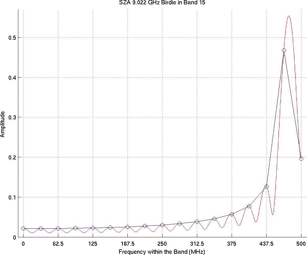
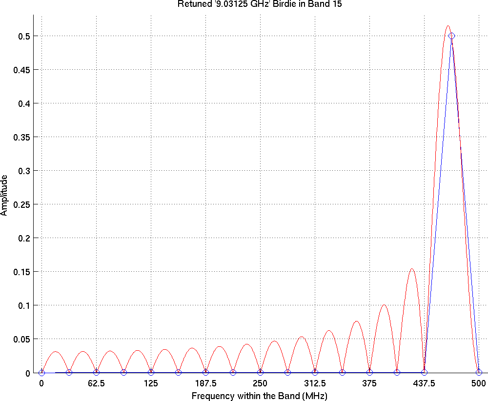
4 Example of Spectral Leakage Corrupting a Band

The 9.022 GHz birdie, arising from the 3${}^{\text{rd}}$ YIG harmonic (detailed at the beginning of this section, §1), corrupted all of Band 15 during initial testing of the SZA (see Table 1). Just before digitization, this birdie is at 1.022 GHz; this is not a discrete multiple of a 500/16 MHz = 31.25 MHz. The birdie’s presence in the final data product (before the problem was solved) indicates that the bandpass filters of the block downconverter could not completely eliminate strong signals from outside the band.

Sampling at 1 GHz aliases the birdie to 522 MHz. Due to the Hermitian property of a real signal’s FFT, frequency is reflected about 500 MHz. The 522 MHz birdie therefore appears in the 0–500 MHz band, between Channels 15 and 16 (468.75 and 500 MHz). The effect of spectral leakage, shown in Fig. 2, is calculated by evaluating the DFT expression for $X(k)$ (Eq. 9), where $x(n)$ was a sinusoid at 522 MHz. While the birdie is strongest in the channels adjacent to its real frequency, it remains above 3% of its full power throughout the entire band, rendering the band useless for observations.

A clever retuning of the last downconverter LO (§1) seen by Band 15 avoids contamination of the entire band, localizing the birdie’s power to one channel. The details of this are as follows: The 9.022 GHz birdie first ends up at 978 MHz after mixing with the 10 GHz LO of the block downconverter; it is then mixed with a 2.0 GHz LO (Downconverter Bank 2, in Fig. 20), which places Band 15 at in the 0.5–1.0 GHz band that is input to the digiters. The digitizers therefore see the birdie at 1.022 GHz. We retuned the last LO to 2.00925 GHz, shifting the birdie to 1.03125 GHz. Fig. 3 shows the spectrum that results from this retuning. The result is that birdie’s power only shows up in Channel 16, which is set in the data reduction pipeline to be automatically flagged (§2).

The final solution to the birdie question was to eliminate the birdies at their sources: the YIG oscillators. By wrapping the YIG in Eccosorb^® (see Fig. 17), we found the signal was sufficiently attenuated; this was a temporary solution, since the form of Eccosorb foam used in this test has a tendency to flake and degrade in the field. A more permanent solution was implemented by simply shielding the YIGs in small aluminum boxes. While the retuning of the 2.0 GHz downconverter LO was retained, periodic measurements continue to show that the YIG harmonics do not escape their aluminum housings (though we still flag Channel 16 of Band 15, as this precaution only costs us one of our $16\times 15$ spectral channels).

2 Antenna Cross-talk

In the survey fields, which were all selected to pass close to zenith in order to minimize atmospheric noise, an apparent excess in noise was discovered between adjacent antennae when observing at antenna elevations $\gtrsim 80^{\circ}$. It was recognized that all the antenna positions that allowed this “excess noise” on these short baselines corresponded to positions where the secondary mirror feedlegs on one antenna had direct lines of sight to the feedlegs on the adjacent antenna.

It was further discovered that, with fringe tracking off and the antennae in a position known to produce “excess noise,” the measured phase versus frequency on that baseline (which for blank, untracked sky should be random noise) was strongly wrapping every two channels; this observed “excess noise” was actually a signal due to “cross-talk” between elements of the antennae, and the wrapping was due to the pathlength between the elements involved in the antenna cross-talk. Since each channel is $31.25~{}\text{MHz}$, the measured wrapping corresponded to a delay of 16 nanoseconds (i.e. $2\times 31.25~{}\text{MHz}$), and the position of the antennae was such that the astronomical delay ($T$ in §3) for that pair of antennae was also 16 nanoseconds. This is because projected baseline at the cross-talk maximum position was roughly $480~{}\text{cm}$, or $cT=(3\times 10^{10}~{}\text{cm s}^{-1})\times(16~{}\text{ns})$. Thus the delay used to track astronomical fringes on the baseline formed by the two antennae also flattened the phase of the cross-talk signal, providing a coherent, correlated signal.

Several ways of eliminating this antenna cross-talk were explored. While the precise cause is unknown, it is hypothesized that the feed horn from one antenna could launch a signal that scattered coherently into the other antenna, and the other antenna would do the same in reverse. With fringe tracking on, the delay being sent to an antenna sometimes precisely flattened this phase wrapping, producing strong, correlated amplitudes in the data.

In order to test that the scattering came from the feedlegs of the secondary, a wire mesh was added to the side of one antenna from a pair that exhibited cross-talk. This shifted the cross-talk to higher antenna elevations. We considered building collars for some or all of the antennae in the inner array, but this was determined to be too costly, and the high winds in Owen Valley would make it difficult to maintain. Furthermore, if the collars extended too far, this would increase the risk of collisions between close-spaced antennae, something the SZA was designed not to have.

We then tried adding Eccosorb^® to the feedlegs (see Figure 4). While the absorber did eliminate cross-talk, it also increased the noise in the system, as each feedleg was now radiating at $\sim 300~{}\text{K}$. For comparison, the cluster signals we observe peak at $\sim 10~{}\text{mK}$. This increase in system noise was determined to be unacceptable, as it increased the required integration times.

Figure 4: Photo of the closest pair of antennae (Antennae 3 & 5, see Fig. 7), with the test Eccosorb^® wrapped around the feedlegs. Ultimately, the Eccosorb^® was replaced by crinkled aluminum foil.

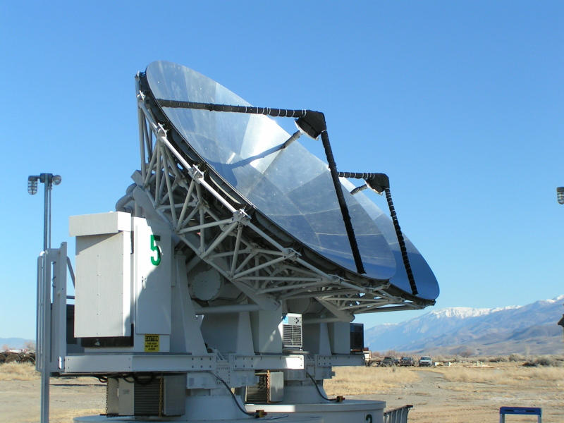
The final solution to the cross-talk problem was to wrap the feedlegs in crinkled, heavy-duty aluminum foil ($\sim$50 mil), available at most grocery stores. The crinkles were carefully constructed to produce large, 3–10 cm facets of arbitrary orientations on the side of the feedleg facing the primary mirror. These facets have the effect of randomly changing the pathlength and angle between corresponding parts of each antenna.

Chapter 3 Data Reduction

In this chapter, I provide a brief overview of the steps necessary to calibrate SZA data. For a more detailed treatment of the SZA data analysis routines, I refer the reader to the thesis of Stephen Muchovej (Muchovej 2008).

The SZA data calibration routine was written by students in the SZA collaboration (primarily Mike Loh, Stephen Muchovej, Matthew Sharp, and Chris Greer) in MATLAB^® code. Since MATLAB^® is a scripting language optimized for matrix manipulation, it is well-suited to manipulate large data sets when performing uniform mathematical operations. Some of the more computationally-intensive routines – in particular, those that required loops – were implemented in external, compiled C/C++ functions that are called from within MATLAB^®. In the following sections, I describe each step in the data reduction pipeline in order of operation

1 System Temperature Computation

The first step in the data calibration routine is a calculation of the system temperature $T_{\rm sys}$ (see Eq. 2). As described in §1, $T_{\rm sys}$ is defined similarly to $T_{\rm rx}$, but accounts for the noise of the entire system scaled to above the Earth’s atmosphere. We therefore use $T_{\rm sys}$ to compute the rms noise level in an observation,

$$\sigma_{rms}\propto\frac{T_{\rm sys}}{\sqrt{N(N-1)\,\tau\,\Delta\nu}}.$$ (1)

Here $N$ is the number of antennae in the array, $\tau$ is the integration time, and $\Delta\nu$ is the bandwidth of the system. For a given integration time, on a given instrument, $T_{\rm sys}$ characterizes the noise in an observation.

Figure 1: System temperatures of a typical SZA cluster observation, computed for each band. One representative antenna is shown, since the other seven all have similar system temperatures. The $y$-axis shows $T_{\rm sys}$ in K, and the $x$-axis is time in hours from the start of the observation. The dark blue point at the start of the observation is the $T_{\rm sys}$ of the bandpass calibrator (§1). The black points are the $T_{\rm sys}$ for the target data (usually a cluster), and the orange points are $T_{\rm sys}$ for the phase calibrator (§2). The points differ due to the differing columns of atmosphere to each source. The minimum in each curve occurs when the source transits (reaches its highest elevation in the sky, and therefore the optical depth reaches its minimum for the observation).

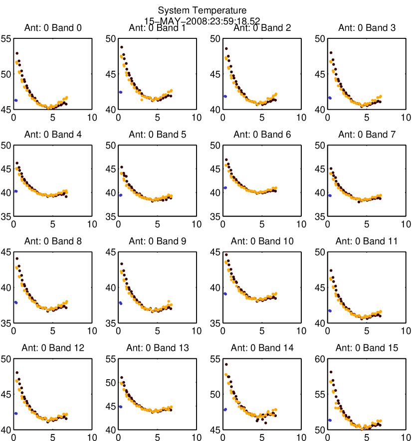
During a typical cluster observation, we compute the noise temperature while observing the phase calibrator and while observing the target (usually a cluster) separately, since each is observed through a different column of atmosphere. See Fig. 1 for a plot of $T_{\rm sys}$ in an observation.

Since $T_{\rm sys}$ is used to compute the theoretical rms noise in the observation at a later stage of the reduction pipeline (see §4), we interpolate our $T_{\rm sys}$ measurements past large deviations from ideal behavior. This ideal noise is used in flagging data that show large deviations from the theoretical rms noise. A jump in $T_{\rm sys}$ of more than $\sim$ 1.5 K can indicate a sudden change in weather or an instrumental effect, so we flag and interpolate stable $T_{\rm sys}$ measurements past these jumps. Additionally, data are flagged if no $T_{\rm sys}$ measurements are available for over $\sim$ 30–35 minutes. This was determined during pipeline testing to be the longest reasonable time to go without a $T_{\rm sys}$ measurement, as we are effectively interpolating the behavior of the atmosphere between actual measurements.

2 Automatic Flagging

Some bad data are next automatically flagged, without any user intervention, on a number of conditions. These conditions can depend on the state of the array, in which case they are flagged by the control system (i.e. for these instances, the reduction routine simply propagates the flags set by the control system). Examples of the common flags set by the control system are:

• Tracking (physical): If a telescope is not mechanically tracking a source for any reason (hardware malfunction, an antenna is off-line for repair, etc.), data from that antenna are flagged.

• Fringe Tracking: If the software that implements fringe tracking (§3) is not functioning properly while observing an astronomical source, there can be no correlated data. Therefore, these data are flagged.

• Correlator Bands not received: If the correlator software is not running for a given band, no correlated data are returned in that band; that band will be flagged.

Other automatic flags can be due to properties of the array that can either be computed or have been measured. These are:

• Antenna Shadowing: For given antenna positions and primary mirror sizes, in a homogeneous array like the SZA, it is straightforward to compute whether one antenna obstructs the view of another. We use a projected antenna spacing of 3.6 meters, which treats the effective primary diameter also as 3.6 m in this calculation (recall that the SZA primary diameter is 3.5 m). This buffer is used to avoid diffraction effects at the edges of the primaries, which are due to the sidelobes of the antenna beam pattern (see Fig. 2). If an antenna is shadowed, all data from that antenna are flagged during that period (i.e. we flag each baseline involving the shadowed antenna for the entire time it is shadowed).

• Birdies: As discussed in §1, radio interference was found to contaminate some of the channels in our observations. A list of bad channels was kept with the rest of the data reduction code, in a Concurrent Versions System (CVS) archive.

• Cross-talk: As discussed in §2, coherent signals between closely-spaced antennae could corrupt baselines. Baselines measured to have significant amounts of cross-talk were noted in the CVS, and those corrupted baselines were excluded.

After the automatic flagging, a baseline correction is applied to the data. By applying small corrections to the antenna locations used by the control system, slightly different astronomical delays are computed for each antenna as the source traverses the sky. The set of correct antenna locations, which produce a constant phase versus time on each baseline, is called the “baseline solution.”

We typically measure the baselines every two weeks by observing many point sources across the sky over the course of a few hours, and permuting the old baseline solution to find the flattest phases for the set of point sources. Common reasons for changes to the baseline solution, which are typically less than a millimeter, involved expansions and contraction of the ground due to rain, or freezing and thawing of moisture in the soil between the concrete antenna pads. No flagging is performed when the baseline solution is applied, as this is simply a mathematical correction that is applied to the data.

3 Interactive Data Calibration

The next step in the pipeline is a series of calibrations that can be run interactively or by specifying scripts with desired parameters on which to flag. While the following steps are now generally run in an automated fashion using scripts supplied by the user, we retain the flexibility to flag data by hand. This manual mode of flagging was particularly important when testing and debugging the pipeline, and was necessary to establish reasonable limits to use in script-driven data calibration.

1 Bandpass calibration

Any component – an amplifier, a cable, a filter, or a mismatch between components or sections of waveguide – can add a spectral shape to the signal that is non-astronomical in origin. By observing an astronomical source known to have a simple power law spectrum, instrumental phase and amplitude features can be calibrated out of the data. Bandpass calibration is done by solving for the corrections necessary to flatten both the amplitude and phase of each band’s spectrum, on a per antenna basis. Since these instrumental features do not change on the timescales of the observation (and typically only do change when a component in the receiver or back-end electronics is changed), the bandpass calibration is performed once per observation, and can often be shared between adjacent observations.

The first interactive flagging step is therefore the bandpass calibration, in which the shape of the instrument’s frequency response is removed from the channel-based data before averaging the bands. Recall from §1 & 2 that there are 15 channels in each of the 16 bands. Data are bandpass calibrated using an $\approx 10$ minute integration on a strong point source ($\gtrsim 10~{}\rm Jy$). This short bandpass calibration observation is taken once per observation, at either the start or finish of an observation (“track”).

Figure 2: Amplitude vs frequency channel of the bandpass calibrator, measured for each band of Antenna 5, before calibration. The $y$-axis is the amplitude in Jy, and the $x$-axis is the channel number. Fig. 4 shows the calibrated amplitude of the bandpass.

Figure 3: Phase vs frequency channel for the bandpass calibrator, measured for each band of Antenna 5, before calibration. The $y$-axis is the phase in degrees, and the $x$-axis is the channel number. Fig. 5 shows the calibrated amplitude of the bandpass.

Figure 4: Amplitude (vs frequency channel) of the bandpass calibrator for each band of Antenna 5, after calibration. See Fig. 2, which shows these bandpass amplitudes pre-calibration, for caption.

Figure 5: Phase (vs frequency channel) of the bandpass calibrator for each band of Antenna 5, after calibration. See Fig. 3, which shows these bandpass phases pre-calibration, for caption.

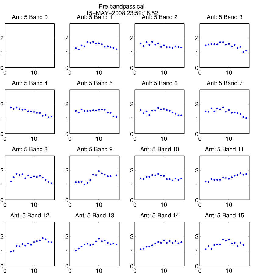
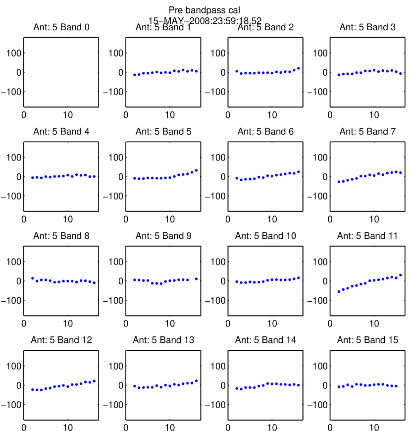
Figures 2 & 3 show the bandpasses for each band of Antenna 5’s amplitude and phase, respectively, before calibration. Figures 4 & 5 show these bandpasses after calibration. After the bandpass calibration has been applied, the channels of each band are binned, and we no longer work with the channel-based data. This binning reduces the size of the dataset by a factor of 17 (see Table 2).

2 Phase/Amplitude calibration

The next step in the calibration corrects for drifts in the overall amplitude and phase of each band. Every $\sim 15$ minutes, a moderately strong ($\gtrsim 2~{}\rm Jy$) point source is observed for 3–5 minutes. An unresolved source at the array’s pointing center (i.e. at the spatial location $(0,0)$) is mathematically a 2-dimensional Dirac delta function, $\delta(0,0)$. Therefore, its spatial Fourier transform is a purely real constant, which implies that each baseline ideally would measure the same amplitude, with zero phase. Deviations from zero phase, therefore, are tracked and corrected using this source as a “phase calibrator.”

Figure 6: Phase of the point source calibrator versus time, as measured by a short baseline (Baseline 0-1). The $y$-axis is the phase in degrees, and the $x$-axis is time in hours since the start of the track. Band 0 was entirely flagged for this track, due to broken digitizers and a lack of spares at the time. The magenta points are those flagged due to the automatic flagging, and the green points are those flagged by a user-specified script’s limits, which catches 30^∘ outliers from the underlying, interpolated phase.

Figure 7: Phase of the point source calibrator versus time, as measured by a long baseline (Baseline 5-6). See Fig. 6 for further details. Note the slightly larger scatter in the phase on this baseline than on Baseline 0-1 (Fig. 6). This is due to atmospheric coherence being slightly poorer on long baselines (the antennae are looking through different columns of air, and atmospheric turbulence has a scale size on the order of tens of meters). The underlying slope in the phase calibrator is easily determined in this observation, as the atmospheric coherence for the example track was typical of a clear spring day.

Figure 8: Amplitude of the point source calibrator versus time, as measured by a short baseline (Baseline 0-1). The $y$-axis is the amplitude in Jy, and the $x$-axis is time in hours since the start of the track. Since a point source is unresolved (the beam is larger than the point source), the amplitude in Jy equals that in Jy/beam. This is the amplitude of the calibrator corresponding to the phase shown in Fig. 6.

Figure 9: Amplitude of the point source calibrator versus time, as measured by a long baseline (Baseline 5-6). This is the amplitude of the calibrator corresponding to the phase shown in Fig. 7. See Fig. 8 for further details.

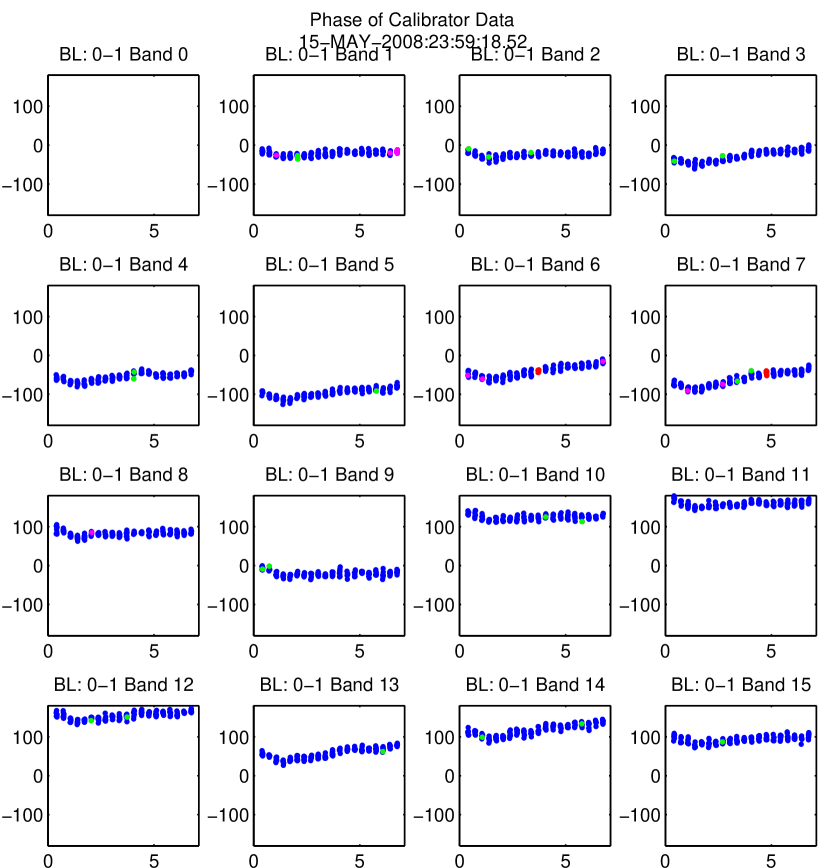
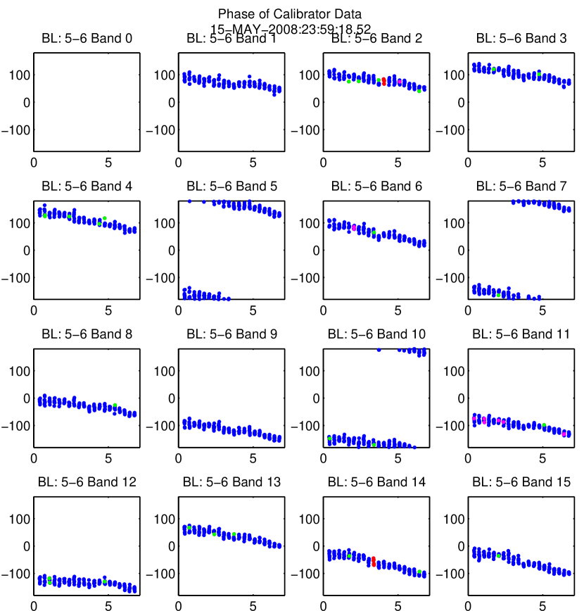
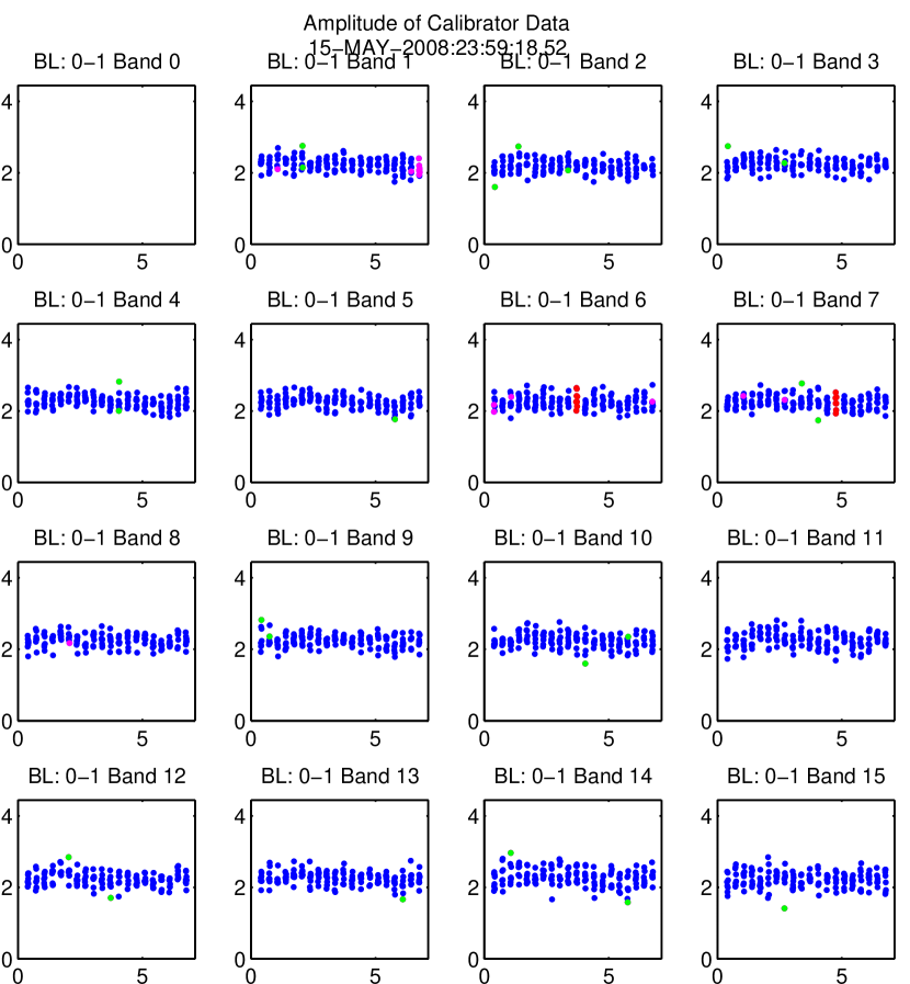
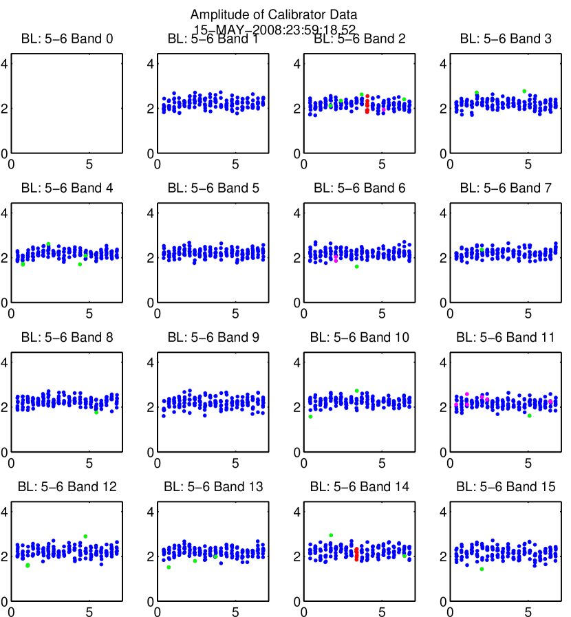
Figures 6–9 show the baseline-based phases and amplitudes of the phase calibrator, measured by the example Baselines 0-1 and 5-6. By setting one antenna per band as the “reference antenna,” which for that band is assumed to have zero phase, the calibrator phase for every other antenna can be computed. The reference antenna for each band is simply chosen to be the first antenna with no flagged calibrator data. In Fig. 11, it is clear – from the flat phase that is identically equal to zero – that Antenna 0 was used as the reference for all bands except Bands 6 & 7, which had flagged phase calibrations mid-track (see red points in Fig. 6).

The phase calibrator is used to track changes in the complex antenna-based gains throughout the track , which can happen for a number of reasons (see Figures 10 & 11). The SZA receivers are well-characterized and have stable gains under normal operating conditions; changes in the complex gain of the actual instrument therefore usually arise when equipment is thermally unstable (failed refrigerator, poor regulation of the electronics box, rapid heating/cooling of the correlator trailer during sunrise/sunset, etc.). Sharp changes in phase, which lead to degradation of the measured amplitude, are used to flag data.

Figure 10: Antenna-based gain of the point source calibrator versus time, for Antenna 0. The $y$-axis is the gain (ideally 1), and the $x$-axis is time in hours since the start of the track. The scatter seen here, which is simply due to noise in the measurement, is smaller than our absolute calibration uncertainty ($\sim 5\%$, see Muchovej et al. (2007)).

Figure 11: Antenna-based phase of the point source calibrator versus time. One antenna must be chosen as a reference in order to compute the antenna-based phase of the other antennae. In this plot, Antenna 0 served as that reference for all but Bands 6 & 7, which had flagged calibration observations (see red points in Fig. 6)

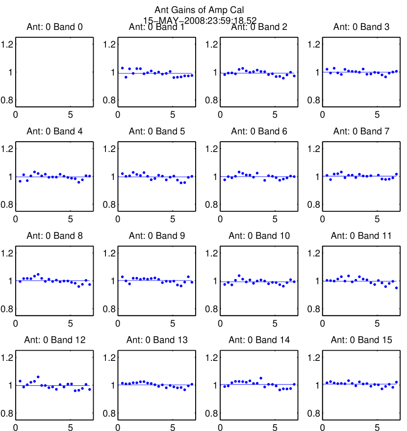
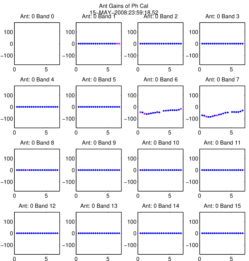
Scatter in the phase due to poor atmospheric coherence can lead to a lower measured amplitude in the correlated data. Clouds and atmospheric turbulence during inclement weather are generally of a small enough scale that a baseline in the inner array measures the full amplitude of the calibrator, as the phase scatter is common-mode on short baselines (i.e. they see the same fluctuations); during such a period, long baselines measure a diminished signal, since the atmosphere is essentially adding random, uncorrelated phase fluctuations to each signal. The example observation presented throughout this chapter was taken on a clear spring day with good atmospheric coherence.

Figure 12: Orphaned data from Antenna 0. Automatically flagged data in Band 0 are shown as green points, and were due to a digitizer hardware problem (and a temporary lack of replacement digitizer boards). Data orphaned by gaps in the calibrator data in Bands 1, 6, & 7 are shown in red (see Fig. 11). Useful data are represented as blue points. For simplicity, target data are plotted with zero phase (rather than plotting the noisy distribution of raw target data phases, since we are only trying to determine which data are not bracketed by calibrator observations). The antenna-based phases of bracketing calibration observations are shown as black X’s (which are identically zero in bands where Antenna 0 was the reference; see Fig. 11).

Figure 13: Orphaned data from Antenna 5. Data orphaned by gaps in the calibrator data in Band 2 are shown in red (see Fig. 7). See Figure 12 for details. Note that Antenna 5 was not the reference antenna for any band in the antenna-based phase calculation, so none of its phases are identically zero.

3 Orphaned data

After phase calibration is complete, periods when data are not bracketed by $T_{\rm sys}$ or phase calibrator observations are flagged, as those data cannot be calibrated. We call these data points “orphans” and discard them. This includes data orphaned by flagged calibrator observations (such as the red points in Figures 6 and 7). Note that this step is antenna-based, since data are typically orphaned by antenna-specific problems (e.g. an antenna was shadowed, or was not tracking and missed a phase calibrator observation). See Figures 12 & 13 for plots that show the flagging of orphaned data.

4 Noise and variance of the data

The next step in the user-guided calibration is to flag target data with a high or biased level of rms noise. The real rms noise of the target data is compared with the expected theoretical value, computed using the measured values of $T_{\rm sys}$ (see §1, Eq. 1). If the variance of the data does not agree with the theoretical value on the $\sim 35\%$ level, the data are flagged. This threshold was determined by Matthew Sharp in a series of jackknife tests (differencing of essentially blank fields) on many CMB fields. Since $T_{\rm sys}$ data have been cleaned of outlier measurements, this flags periods with higher than expected noise.

Figure 14: rms of target data, taken on short Baseline 0-1. The theoretical prediction, based on the measured $T_{\rm sys}$, is shown in black. Flagged data – already caught by other steps (see Figures 6 & 12 in particular) – are plotted in red and magenta. Newly flagged data are in green. Useful, unflagged data are in blue.

Figure 15: rms of target data, taken on long Baseline 5-6. Flagged data – already caught by other steps (see Figures 7 & 13) – are plotted in red and magenta. See Figure 14 for more details.

Additionally, any data points with more than a 4-$\sigma$ deviation from the distribution are flagged. While this filter is useful in principle, data with such large error bars are typically caught in the previous steps. See Figures 14 & 15 for plots of the rms noise of target data for a long and a short example baseline.

The expected rms noise is computed using cleaned $T_{\rm sys}$ data, where any jumps in $T_{\rm sys}$ have been interpolated past. However, if the jump was due to a real instrumental or atmospheric effect, the data will show a similar jump in measured rms noise. This is why large deviations from the expected theoretical noise are flagged. An example of an instrumental effect that leads to a higher than expected rms level (without affecting the measured $T_{\rm sys}$) is antenna cross-talk, discussed in §2.

5 Amplitude of the target data

The last step of user-guided calibration flags for anomalies in the amplitude of the raw target data. For the example cluster observation (shown in Figs. 16 & 17), there are no strong ($\gtrsim 1~{}\rm Jy$) point sources in the field. Individual data points are dominated by noise, since the cluster signal is on the order of ten mJy (total, integrated over the sky), and the rms noise per second is $\sim 0.5~{}\rm Jy/beam$. Data points with more than a 4-$\sigma$ deviation from the mean – which could be due to high atmospheric noise – are typically flagged. Also, any jumps in target amplitude are immediately suspect, as they are indications of undesired instrumental/atmospheric effects (since the cluster SZE signals and point source fluxes are not time-dependent on the scale of hours).

Figure 16: Amplitude of visibility data (in Jy, see §3) for a short baseline (0-1), taken on the target source (typically a cluster). Blue points are unflagged data. Red and magenta points are flagged data caught by previous steps in the data calibration (see Figures 6 & 12), while green points may indicate data flagged in this step as outliers or from previous steps (e.g. Bands 1, 2, & 14 contain some green points that are not outliers, flagged in Fig. 6). The SZE flux from the cluster and the fluxes of point sources in the cluster field are on the $\sim$ mJy level; they are therefore not noticeable in the raw data plotted here (which are noise dominated).

Figure 17: Amplitude of visibility data in Jy (see §3) for a long baseline (5-6) taken on the target source. See Fig. 16. Note that long baselines do not typically measure cluster scales, but the raw target data here and in Fig. 16 have similar amplitudes. Also note that some green, flagged points (e.g. in Band 13) were flagged in Fig. 7, not because they are outliers.

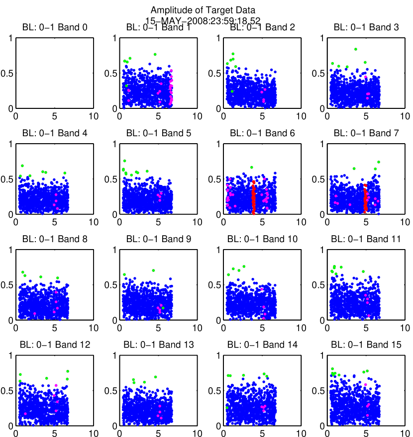
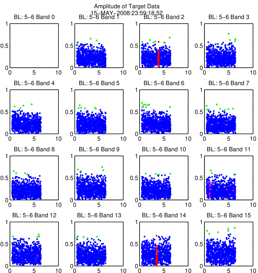
Though we never attempted observations of clusters with ($\gtrsim 1~{}\rm Jy$) point sources in the field, the CMB and cluster survey data often do contain such sources. Their presence simply raises the mean value of the amplitude of the target data. Since we only flag on outliers from the distribution, note that this step does not prevent us from performing observations of fields with strong point sources.

4 Dirty Maps

After all steps of the calibration are complete, the machinery of Difmap (Shepherd 1997), imported into MATLAB^®, is used to produce rudimentary maps of the observation (shown in Fig. 18). These maps are largely illustrative, as all quantitative results of the SZE cluster observations are determined by fitting the visibilities in u,v-space (see §4). We do this because the noise properties of the visibilities in u,v-space are well understood.

In Fig. 18, the short baseline data (upper panel) show a central, dark blue “blob,” which is the flux decrement due to the cluster CL J1226.9+3332. To the left of the cluster, which is east on the sky, a $\sim 4~{}\rm Jy$ source is seen as a red “blob” (attenuated by the primary beam to $\sim 2.5~{}\rm Jy$, as it is $4.5\arcmin$ from the center). The resolution of the upper panel map is determined by the scale probed by the short baselines, and not the size of the source in the sky (if larger, the baseline would not be sensitive to the source). The lower panel shows a slight excess in flux at the point source position. The long baselines do not probe cluster scales. For well-calibrated data, only the very strongest sources show up in a single track, and a typical cluster observation requires more than a single track to constrain a cluster’s SZE signal (as well as the weak $\sim$ few mJy point sources in the field). We therefore expect a single track to be dominated by noise.

Figure 18: Dirty maps of the short (upper panel, $\lesssim 2~{}\rm k\lambda$) and long (lower panel, $\gtrsim 2~{}\rm k\lambda$). $x$ and $y$ axes are the map coordinates in degrees. The colors represent the signal in Jy/beam (the flux detected within the beam formed by each baseline). See text for more details.

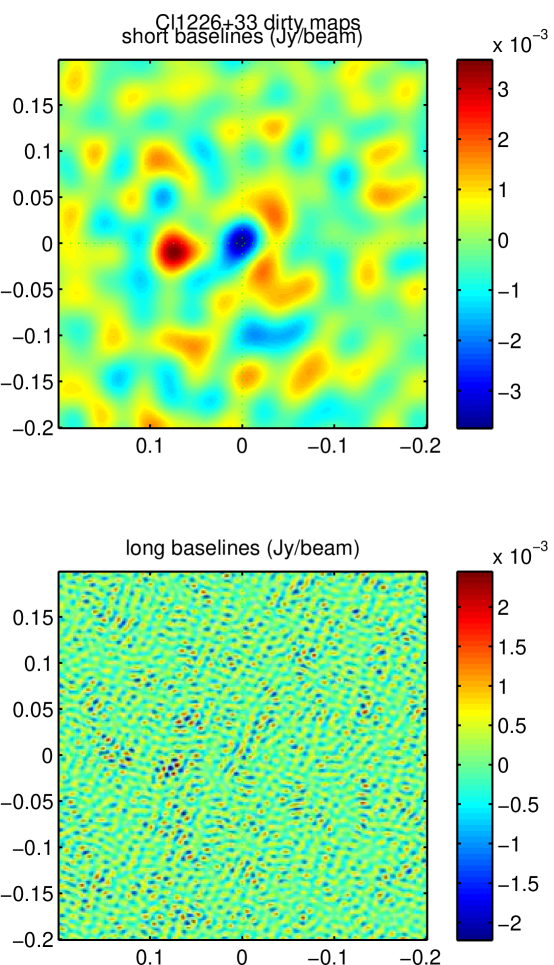
5 Final Data Product

Calibrated data are output, using a C++ function written by Erik Leitch, in the standard Flexible Image Transport System (FITS) format for astronomical data. Since these are radio interferometric data in u,v-space, we use the UVFITS specification of the FITS format. These files contain the real and imaginary components of the visibility data (in Jy, see §3) from all 16 SZA bands, stored in binary format. They also contain the u,v-space coordinates and weights (inverse variance, 1/$\sigma_{\text{rms}}^{2}$) for each data point.

Further useful information is also stored in the UVFITS file. An ASCII header provides observation specifics, such as the date of the observation, name of the observatory, name of the target observed, the pointing center used for the target, and the frequency at which it was observed, while a binary table includes each antenna’s physical location.

Part 2 Modeling and Analysis of Clusters

Chapter 4 Modeling the Cluster Signal

1 Introduction to Cluster Models

As detailed in §2, the SZA interferometer probes a cluster’s SZE signal in u,v-space (see Figures 5–11). In order to extract physical parameters from an interferometric cluster observation, we need to fill in information on the scales we do not probe. A simple model to extrapolate through the individually noisy, sparsely-sampled visibilities (Eq. 6), is used to extract meaningful constraints on physical cluster parameters. Given the large gaps in the u,v-coverage, a simple, 2-parameter model was found to work best.

When fitting data in u,v-space, it is helpful to consider two extreme cases: scales below the resolution of the instrument (i.e. smaller than the scales probed by the longest baseline), and scales larger than the shortest baseline probes. The first case defines what we consider to be a point source, where in u,v-space each antenna ideally measures constant, uniform power.

The second case implies that we are not sensitive to backgrounds, such as the primary CMB (most of its power is on much larger angular scales than we probe) or large-scale galactic emission (from our galaxy). This makes the SZA a good spatial filter for clusters at high redshift, since it interferometrically probes Fourier modes of the spatial intensity pattern corresponding to the bulk of a cluster’s signal. It also means we cannot constrain cluster features on scales larger than the shortest baseline can probe. A cluster model can predict an arbitrary signal at scales larger than we can probe; a poorly-motivated model can have Fourier modes in its transform that agree with the measured SZE signal, but might predict too much or too little flux on scales not accessible to an interferometer. At the longest wavelength of the SZA, observing down to the shadowing limit, this upper limit is $\approx 12.7\arcmin$; above this scale, information is lost due to lack of u,v-coverage.

Modeling of any signal, including that due to the SZ effect in clusters, introduces priors on the resulting fit and its derived quantities. I discuss below the SZE models I tested, as well as the X-ray models used to complement them. I then discuss the Markov chain Monte Carlo (MCMC) fitting procedure we use to fit these models jointly to SZE+X-ray data. Finally, I show how we derive galaxy cluster properties from the resulting model parameters.

Throughout this section, we use several common cluster overdensity radii that appear often in the literature. These overdensity radii are defined with respect to the critical density of the Universe $\rho_{c}(z)$ at the cluster’s redshift (see Eq. 35). We define $r_{\Delta}$ as the radius within which the average (gas+dark matter) density is $\Delta\,\rho_{c}(z)$ (e.g. $r_{2500}$ is the radius containing an overdensity $2500\rho_{c}(z)$, and $r_{500}$ is the radius containing $500\rho_{c}(z)$). Since the mean cluster density drops with radius, a smaller overdensity $\Delta$ corresponds to a larger radius. A good rule of thumb is that $r_{500}\approx 2\,r_{2500}$ for most massive clusters. We show how we solve for these radii for real observations in §6.

2 $\beta$-Model SZE Profiles

1 The $\beta$-model

The $\beta$-model, also called the King profile, has a long history (Cavaliere & Fusco-Femiano 1976, 1978) of performing remarkably well at parameterizing cluster radial gas density profiles. Part of its appeal is its simplicity. Here I show how to derive the line of sight Compton $y$ parameter when a $\beta$-model is used to describe the radial electron pressure profile,

$$P_{e}(r)=P_{e,0}\left[1+(r/r_{c})^{2}\right]^{-3\beta/2}.$$ (1)

Here $P_{e,0}$ is the central electron pressure, $\beta$ is a single slope that describes how pressure decreases with radius, and $r_{c}$ is the “core radius,” typically $\sim$ 100 kpc for a massive cluster. For $\beta=2/3$ – a typical value when this model is used to describe the intra-cluster medium’s (ICM) density – $r_{c}$ is the radius at which the electron pressure falls to half its central value.

Figure 1: Geometry for the line of sight integral of a spherically-symmetric model.

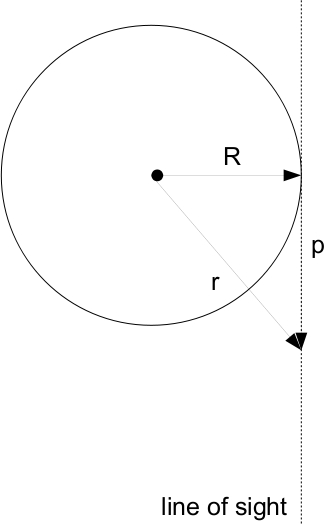
Figure 1 shows the geometry for the line of sight integral of a spherically-symmetric ICM model. Here, $\vec{r}$ is the radius within the cluster, $R$ is the radius on the sky (from the projected cluster center on the sky), and ${p}=\sqrt{\vec{r}\,^{2}-R^{2}}$ is the distance along the line of sight. The radius on the sky, $R$, is a constant in the integration, equal to the minimum in $\vec{r}$ (see Figure 1). The Compton $y$ parameter as a function of $R$ is

$$y(R)=\frac{\sigma_{T}}{m_{e}\,c^{2}}\int_{-\infty}^{\infty}P_{e,0}\left[1+({r}/r_{c})^{2}\right]^{-3\beta/2}\frac{{r}}{\sqrt{{r}^{2}-R^{2}}}\,d{r}.$$ (2)

Substituting in ${p}$ and $d{p}/d{r}={r}/\sqrt{{r}^{2}-R^{2}}$, and taking advantage of the symmetry, we have

$$y(R)=2P_{e,0}\frac{\sigma_{T}}{m_{e}\,c^{2}}\int_{0}^{\infty}\left[1+({p}/r_{c})^{2}+(R/r_{c})^{2}\right]^{-3\beta/2}d{p}.$$ (3)

A rearrangement of terms yields

$$y(R)=2P_{e,0}\,\frac{\sigma_{T}}{m_{e}c^{2}}\,\left[1+(R/r_{c})^{2}\right]^{-3\beta/2}\int_{0}^{\infty}\left\{1+\frac{{p}^{2}}{r_{c}^{2}[1+(R/r_{c})^{2}]}\right\}^{-3\beta/2}\!\!dp.$$ (4)

Defining the quantity $p_{c}=\sqrt{r_{c}^{2}+R^{2}}$, the integral in Eq. 4 becomes integrable in terms of the hypergeometric Eulerian function $\Gamma$.

$$\begin{split}\int_{0}^{\infty}\left\{1+\frac{{p}^{2}}{r_{c}^{2}[1+(R/r_{c})^{2}]}\right\}^{-3\beta/2}\!\!d{p}=\int_{0}^{\infty}\!\left[1+(p/p_{c})^{2}\right]^{-3\beta/2}dp\\ =\sqrt{\pi}\,p_{c}\,\frac{\Gamma(3\beta/2-1/2)}{\Gamma(3\beta/2)}\\ =\sqrt{\pi(r_{c}^{2}+R^{2})}\,\frac{\Gamma(3\beta/2-1/2)}{\Gamma(3\beta/2)}\\ =\sqrt{\pi}\,r_{c}[1+(R/r_{c})^{2}]^{1/2}\,\frac{\Gamma(3\beta/2-1/2)}{\Gamma(3\beta/2)}\end{split}$$ (5)

Putting the result of Eq. 5 back into Eq. 4, we finally have

$$y(R)=2P_{e,0}\,\frac{\sigma_{T}}{m_{e}c^{2}}\,\sqrt{\pi}\,r_{c}\,[1+(R/r_{c})^{2}]^{-3\beta/2+1/2}\,\frac{\Gamma(3\beta/2-1/2)}{\Gamma(3\beta/2)}$$ (6)

Note that Eq. 6 has the same form as the integral of the line of sight through the center of the cluster. We therefore can define the central Compton $y$ parameter $y_{0}$:

$$y_{0}=2P_{e,0}\,\frac{\sigma_{T}}{m_{e}c^{2}}\,\sqrt{\pi}\,r_{c}\,\frac{\Gamma(3\beta/2-1/2)}{\Gamma(3\beta/2)}.$$ (7)

This yields the expression for the SZE $\beta$-model commonly fit to observations:

$$y(R)=y_{0}\,[1+(R/r_{c})^{2}]^{-3\beta/2+1/2}.$$ (8)

In terms of temperature decrement $\Delta T/\mbox{$T_{\mbox{\tiny CMB}}$}=f(x)\,y$ (as in Eq. 1), we also define the central decrement

$$\Delta T_{0}\equiv f(x)\,y_{0}\,\mbox{$T_{\mbox{\tiny CMB}}$},$$ (9)

where $f(x)$ contains the frequency dependence of the SZE (see Eq. 4).

The $\beta$-model thus provides a simple, semi-analytic formula for fitting SZE data.

2 The Isothermal $\beta$-model

In §1, we made no assumptions about the temperature, density, or metallicity distribution within the ICM; we only assumed the electron pressure can be described by a $\beta$-profile.

For the following, we make the common assumption of isothermality. We will also assume the X-ray-determined isothermal spectroscopic temperature $T_{X}$ is the temperature of the ICM gas ($T_{e}(r)=T_{X}$). Using Eq. 1 and applying the ideal gas law,

$$P_{e}=k_{B}\,n_{e}\,T_{e},$$ (10)

we arrive at this expression for the electron density:

$$n_{e}(r)=n_{e,0}\left[1+(r/r_{c})^{2}\right]^{-3\beta/2}.$$ (11)

A number of joint SZE+X-ray cluster studies have been performed using the isothermal $\beta$-model (see, for example Grego 1999; LaRoque et al. 2006; Bonamente et al. 2008). Throughout these studies, the isothermal $\beta$-model has been applied in various ways; for simplicity we only discuss the most recent. In LaRoque et al. (2006) and Bonamente et al. (2008), the jointly-fit SZE and X-ray data were used to constrain an SZE-determined central electron density, $n_{e,0,SZ}$. This comes from applying Eq. 10 to the SZE-constrained central pressure $P_{e,0}$, and using the X-ray-constrained temperature $T_{X}$ to solve for the central density (i.e. They used $n_{e,0,SZ}=P_{e,0}/k_{B}T_{X}$). The analogous X-ray-determined central electron density, which does not require SZE data, is called $n_{e,0,X}$ in this context (and later is just called $n_{e,0}$, as we never use $n_{e,0,SZ}$ in this work). By not requiring $n_{e,0,SZ}=n_{e,0,X}$ to hold when jointly fitting SZE+X-ray data, the central decrement (Eq. 9) can be allowed to fit freely the amplitude of the SZE signal. These different normalizations for the electron density profile were used to provide somewhat independent constraints on the hot gas fraction, using the X-ray-constrained estimate of the total cluster mass with the X-ray or SZE-constrained gas mass estimates (we show how these quantities are derived from the fit profiles in §5). An important drawback of this method is that, since X-ray imaging data have a much higher spatial significance than SZE data, the jointly-fit shape parameters $r_{c}$ and $\beta$ are driven to those values preferred by the X-ray data (as we will demonstrate in §6). Furthermore, it has been well-established by X-ray observations that isothermality is a poor approximation both within the cluster core and at large radii (see e.g. Piffaretti et al. 2005; Vikhlinin et al. 2005; Pratt et al. 2007, and references therein)).

Since current X-ray imaging data have higher signal to noise than current SZE observations, and X-ray imaging has been shown to recover well cluster gas density (Nagai et al. 2007b), we will instead only consider, for comparison, what the SZE fit yields for SZE-specific quantities, such as electron pressure and the integrated, intrinsic Compton-$y$ parameter, $Y_{\mbox{\scriptsize int}}$ (see §1). We use the X-ray-determined density and temperature for all other quantities derived from cluster observations that have been fit with the isothermal $\beta$-model, and do not attempt to constrain electron density with SZE data.

As noted above, the assumption of isothermality does not remain valid over a broad radial extent of a cluster, even when the core is excluded from the X-ray data (as was done in LaRoque et al. (2006) and Bonamente et al. (2008), for example). Early joint SZE+X-ray data fitting only allowed the SZE data to constrain one unique parameter – $y_{0}$ – to within $\sim 10\%$ error bars, while X-ray data primarily constrained the cluster shape parameters ($\beta$ and $r_{c}$, used to fit both the SZE and X-ray data) and density normalization $n_{e,0}$. Since the SZA can integrate to the OVRO/BIMA signal levels $\sim 8$ times more quickly, the resulting higher quality data of a typical 30-GHz SZA observation allows two parameters to be uniquely determined by SZE data. An additional benefit of the SZA over OVRO/BIMA is in the shorter baselines, due to the close-packed inner array (discussed in §1). The short baselines of the SZA allow us to probe larger scales, where isothermality is not expected to hold.

Note that we present the results of the isothermal $\beta$-model jointfits for comparison only, and use its limitations to demonstrate how a new model, presented next, can move beyond the $\beta$-model.

3 A New SZE Pressure Profile

1 Motivations for a New Pressure Profile

We motivate here the use of a new pressure profile, chosen not to have shape parameters linked to those used in fitting the X-ray imaging data, which primarily determine ICM density (note the $n_{e}^{2}(r)$ dependence in Eq. 8 for the X-ray surface brightness implies a strong density dependence). By chosing a new pressure profile, we explicitly allow the electron pressure and density profiles, $P_{e}(r)$ and $n_{e}(r)$, to have different shapes, consistent with a non-isothermal electron temperature profile $T_{e}(r)$. In order to motivate this new pressure profile, first presented in Nagai et al. (2007a, hereafter N07), we examine the empirical evidence afforded by recent, detailed X-ray studies of galaxy clusters. It is known that the isothermal assumption does not hold over a broad range of cluster radii (see, e.g., Figure 3). In this section, we discuss some of the background work that provides the foundations of the new models.

In looking at clusters over a broad range of masses, we hope to identify whether or not they exhibit self-similarity, which (if self-similarity holds) implies that they tend toward the same shape or slope when scaled to a fiducial radius such as the virial radius or $r_{500}$. While several works have demonstrated that temperature can exhibit a nearly self-similar decline at large radii ($r>0.2\,r_{\text{vir}}$, see e.g. Loken et al. (2002); Markevitch et al. (1998)), it is also clear in these works and in recent detailed X-ray measurements that cluster temperature profiles are not universal or self-similar over all cluster radii (particularly within the cores; see Vikhlinin et al. (2005, 2006) and Fig. 3).

Figure 2: The above figure shows fits to the density profiles of 11 nearby, relaxed real clusters, as well as to the average density profiles of 16 clusters simulated using adiabatic (red) and cooling + star-formation (blue) physics. V06 motivate the use of a nine-parameter density model (Eq. 12) to model these density profiles. Figure from N07.

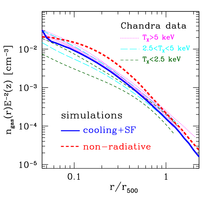
Recently, Vikhlinin et al. (2006, hereafter V06) demonstrated a new density model, which they used to fit the surface brightness profiles of 11 nearby, relaxed clusters of galaxies with deep Chandra X-ray exposures. The density profile V06 fit is

$$n_{e}(r)=\sqrt{\frac{n_{e0}^{2}\,(r/r_{c})^{-\alpha}}{\left[1+(r/r_{c})^{2}\right]^{3\beta-\alpha/2}}\frac{1}{\left[1+(r/r_{s})^{\gamma}\right]^{\varepsilon/\gamma}}+\frac{n_{e02}^{2}}{\left[1+(r/r_{c2})^{2}\right]^{3\beta_{2}}}}.$$ (12)

We refer to this equation as the “V06 density model.” We note that the $\alpha$ component in the first term of Eq. 12 was introduced by Pratt & Arnaud (2002) to fit the inner slope of cuspy cluster density profiles. For $\alpha=0$, the first half of the first term is a $\beta$-model. The second part of the first term – $\left[1+(r/r_{s})^{\gamma}\right]^{-\varepsilon/\gamma}$ – accounts for any steepening around $r_{500}$ observed in these clusters. The additive second term – $n_{e02}^{2}\left[1+(r/r_{c2})^{2}\right]^{-3\beta_{2}}$ – is simply another, smaller $\beta$-model component, which is also present explicitly to fit the cluster core (and is degenerate with the $\alpha$ component of the first term). Of the nine free parameters in the V06 density model, four are present explicitly to fit the inner regions of the cluster ($\alpha,\beta_{2},n_{e02},\&~{}r_{c2}$).

V06 coupled Eq. 12 with a new radial temperature profile, which is

$$T_{\mathrm{3D}}(r)=T_{0}\left[\frac{(r/r_{\text{cool}})^{a_{\text{cool}}}+T_{\text{min}}/T_{0}}{(r/r_{\text{cool}})^{a_{\text{cool}}}+1}\right]\left[\frac{(r/r_{t})^{-a}}{(1+(r/r_{t})^{b})^{c/b}}\right].$$ (13)

This profile has eight free parameters. The term in the first set of square brackets describes any cool core present in the cluster, where the temperature approaches $T_{\text{min}}$ as $r\rightarrow 0$. The term in the second set of brackets describes the decline in temperature in the cluster outskirts, as $r\rightarrow\infty$.

Figure 2 compares the density profiles of the 11 real clusters presented in V06 to those fit to mock X-ray observations of the Kravtsov et al. (2005) sample of clusters; those clusters were simulated separately with adiabatic (‘non-radiative’) and with gas cooling and stellar formation (‘cooling+SF’ or CSF) feedback physics. The figure and analysis of the mock X-ray observations are presented in N07 (I simply use their results here). Note that outside the core ($r>0.15\,r_{500}$), the density profiles of these relaxed clusters have slopes that are more similar than within $r<0.15\,r_{500}$. This can be seen as the gas density profiles of the real clusters with $T_{X}>5~{}\rm keV$ (magenta) and the CSF simulated clusters tend toward roughly the same slopes beyond $r>0.15\,r_{500}$.

Figure 3: The above figure shows fits to the temperature profiles of 11 nearby, relaxed real clusters (in green, magenta, and cyan), as well as to the average temperature profiles of 16 clusters simulated using adiabatic (red) and cooling + star-formation (blue) physics. All profiles are scaled to their best-fit $r_{500}$ values. V06 used the eight-parameter temperature model (Eq. 13) to capture the details of the real cluster temperature profiles. Figure from N07.

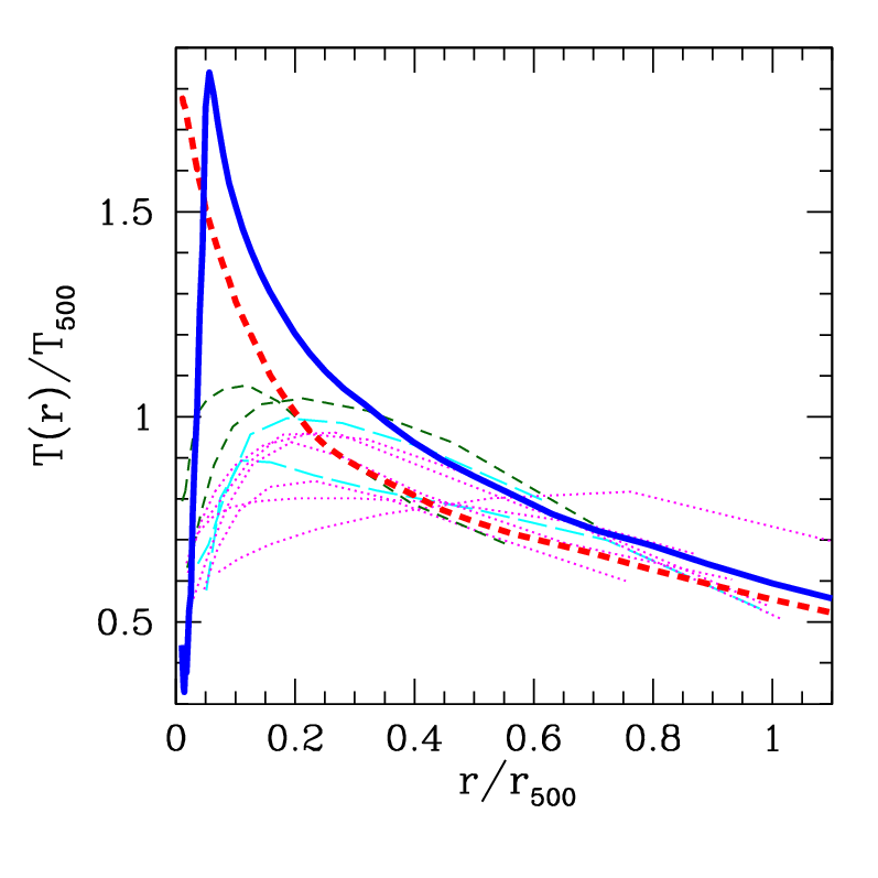
Figure 3 compares the radially-averaged temperature profiles fit to Chandra X-ray spectroscopic data of these same 11 relaxed clusters from V06. It also shows the average temperature profiles of the Kravtsov et al. (2005) simulated clusters. Note in Fig. 3 that the large spike in the temperature profiles of the simulated clusters, accompanied by a sudden drop for the CSF simulations, is generally accepted as evidence that one or more cluster feedback mechanisms is missing from the simulations. The CSF simulations in particular, which exhibit an exaggerated cusp in density (Fig. 2), suffer from this “over-cooling problem.”

2 Generalized NFW Model for ICM Pressure

Figure 4: The above figure shows the X-ray-derived pressure profiles of 5 nearby, relaxed real clusters with $T_{X}>5~{}\rm keV$, as well as to the average 3-D, radially-averaged pressure profiles of 16 clusters simulated using adiabatic (red) and cooling + star-formation (blue) physics. The black lines are the best fit generalized NFW profiles for each type of cluster plotted. Figure from N07.

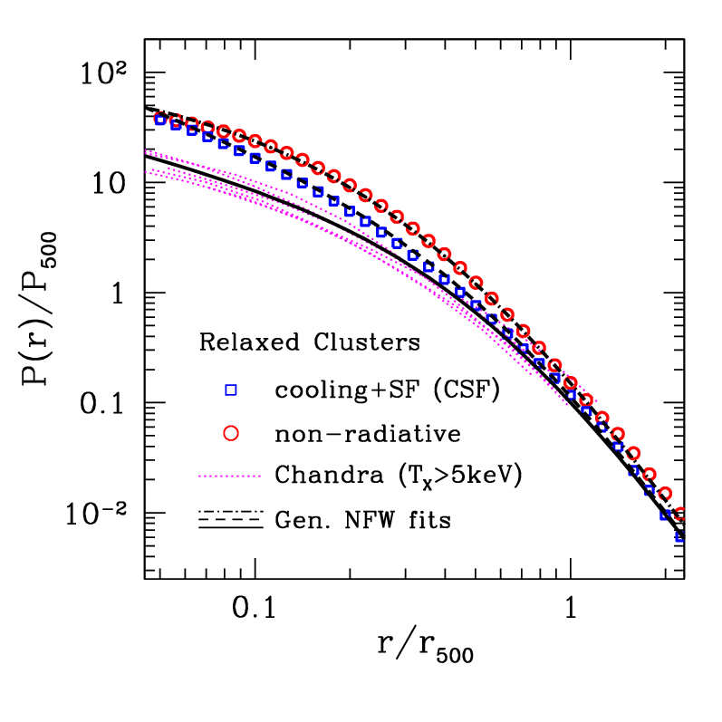
Applying the ideal gas law (Eq. 10) to the density and temperature fits presented in V06, N07 derived the ICM pressure profiles of the V06 relaxed clusters. Additionally, N07 analyzed the 3-D, radially-averaged pressure profiles of their simulated cluster sample (the Kravtsov et al. (2005) sample). N07 found that the pressure profiles of both simulated and real clusters can be accurately described by similar generalizations of the Navarro, Frenk, and White (Navarro et al. 1997, NFW) model used to fit dark matter halos of simulated clusters. Note that the cuspy core was excluded from the analysis in N07, so the over-cooling in the simulations does not affect the conclusions they draw about the derived pressure profile.

The generalized NFW profile (abbreviated “genNFW” for convenience) applied to the electron pressure has the form:

$$P_{e}(r)=\frac{P_{e,i}}{(r/r_{p})^{c}\left[1+(r/r_{p})^{a}\right]^{(b-c)/a}}.$$ (14)

where $P_{e,i}$ is a scalar normalization of the pressure profile, $r_{p}$ is a scale radius (typically $r_{p}\approx r_{500}/1.8$), and the parameters $(a,b,c)$ respectively describe the slopes at intermediate ($r\approx r_{p}$), outer ($r>r_{p}$), and inner ($r\ll r_{p}$) radii; we refer to $(a,b,c)$ as the genNFW “slope parameters.” Note that choosing a pressure profile similar to the dark matter halo’s density profile is reasonable because the gas pressure distribution is primarily determined by the gravitationally dominant dark matter component. As we show in §1, the integral of thermal pressure (ergs/cm³) can be directly related to the (thermal) energy content of a cluster. As the dominant form of kinetic energy in the ICM, thermal energy tracks the underlying gravitational potential – and ultimately the dark matter halo – to the extent that the cluster is in pressure equilibrium (i.e. pressure balances the gravitational pull). It is therefore unsurprising that the pressure profiles of relaxed clusters should be self-similar and have a profile resembling that of dark matter.

It is worth noting that, to derive pressure from the V06 profiles, seventeen parameters (many degenerate) – eight for $T(r)$ and nine for $n_{e}(r)$ – have been fit, while the X-ray derived pressures of all clusters in the V06 sample were well-fit by the five parameters of the genNFW profile (on the percent level). N07 provide best-fit, fixed slopes $(a,b,c)$ for the genNFW profile, which they obtained by fitting both types of simulated clusters as well as the real clusters with spectroscopic temperatures above $5~{}\rm keV$, presented in V06.

The implications of this self-similarity in ICM pressure profile can be understood further by the analysis of cluster dynamical timescales. Since inhomogeneities in pressure propagate as sound waves in the ICM, the sound-crossing time $t_{\rm sc}$ is relevant in determining how rapidly a disturbance in pressure equilibrates. Ettori (2001) provides the sound-crossing time:

$$t_{\rm sc}=1.2\,\left(\frac{10~{}{\rm keV}}{kT_{\rm gas}}\right)^{\!1/2}\left(\frac{R}{1~{}\rm Mpc}\right)\rm Gyrs.$$ (15)

Here $R$ is the scale of a feature out of pressure equilibrium, and $kT_{\rm gas}$ is the feature’s temperature in keV. As an example, a hot subcluster with a temperature of 10 keV and size of 0.1 Mpc merging subsonically with a larger cluster would reach pressure equilibrium with its immediate surroundings in only $\sim 0.12~{}\rm Gyrs$. This is much less than the age of a typical cluster. For such a merging cluster not to be near pressure equilibrium, the merger would have to be very recent, or the subclump would have to be traveling close to the speed of sound.

Some Common Simplifications of the Generalized NFW Model

For different choices of slopes, the genNFW profile reduces to several interesting or familiar cases:

• Dark Matter Halo Profiles: The slopes $(a,b,c)=(1,3,1)$ yield the NFW profile for dark matter halos. Similarly, the genNFW profile reduces to the Moore et al. (1999) profile by setting $(a,b,c)=(1.5,3,1)$, and to the Jing & Suto (2000) profile for galaxy clusters when $(a,b,c)=(1.1,3,1)$.

• The $\beta$-model:: Setting the slopes to $(a,b,c)=(2,3\beta,0)$ reproduces the $\beta$-model, where $b=3\beta$. In this case $P_{e,i}=P_{e,0}$ and $r_{p}=r_{c}$.

• The N07 Pressure Profile: The slopes $(a,b,c)=(1.3,4.3,0.7)$ yield the profile we use in fitting real clusters of galaxies (see the discussion below, in §3).

• The N07 Pressure Profile for Simulated Clusters: A slightly cuspier inner slope, $c=1.1$, yields the best-fit pressure profile clusters simulated with CSF physics. The full set of slopes is therefore $(a,b,c)=(1.3,4.3,1.1)$.

Slope of the Generalized NFW Pressure Profile ($dP/dr$)

We provide here the derivative, with respect to $r$, of the genNFW pressure profile. This will be useful when estimating the cluster total mass, $M_{\mbox{\scriptsize tot}}$, using the equation of hydrostatic equilibrium (Eq. 32, §4).

$$\frac{dP(r)}{dr}=-\frac{P_{e,i}}{r}\left(\frac{r}{r_{p}}\right)^{\!-c}\left[1+\left(\frac{r}{r_{p}}\right)^{\!a}\right]^{-(a+b-c)/a}\left[b\left(\frac{r}{r_{p}}\right)^{\!a}+c\right].$$ (16)

3 The N07 Pressure Profile

In order to reduce the number of free parameters to those that can be constrained by existing SZE observations of clusters, we fix the slopes of the genNFW profile to the best-fit slopes provided by N07, and test their ability to extract cluster physical parameters in Chapter 5. By using these fixed slopes to fit the SZE, we take advantage of the self-similarity of cluster pressure profiles across a broad range of masses. N07 found that the pressure profiles of all sixteen clusters simulated using cooling and star formation physics could be well fit with the slopes of the profile fixed to the same values (namely $(a,b,c)=(1.3,4.3,1.1)$), while the pressure profiles of several relaxed, real clusters, studied in detail using Chandra and presented in V06, could all be fit using a slightly different value for the inner slope, $c=0.7$. Therefore, the pressure profile we test – Eq. 14 with slopes fixed at $(a,b,c)=(1.3,4.3,0.7)$ – becomes

$$P_{e}(r)=\frac{P_{e,i}}{(r/r_{p})^{0.7}\left[1+(r/r_{p})^{1.3}\right]^{3.6/1.3}}.$$ (17)

The clusters simulated with non-radiative, adiabatic physics required quite different slopes, which we do not consider here, due to the simplified physics used in their simulation. As demonstrated by N07, we note that the same outer slope used to fit the V06 (real) cluster and the CSF simulated clusters, $b=4.3$, also fit well the clusters simulated using adiabatic physics.

4 Simplified Vikhlinin Density Model – An X-ray Density Model to Complement the N07 Pressure Profile

The density model we chose for fitting X-ray imaging data is a simplified, core-cut form of the V06 density model. We justify this core cut because we are primarily interested in recovering cluster parameters at $r_{2500}$ and $r_{500}$, where the contribution from the core is negligible. We refer to our simplification as the “Simplified Vikhlinin Model” or “SVM” hereafter. Many have demonstrated (see, e.g. LaRoque et al. 2006) that a core-cut isothermal $\beta$-model recovers $M_{\mbox{\scriptsize gas}}$ accurately outside the inner 100 kpc, out to $r_{2500}$. We chose this simple modification as a suitable description of intermediate-quality X-ray data outside the core, out to, and possibly beyond, $r_{500}$. We note that V06 presented this profile as an intermediate step to obtaining the full 9-parameter density model (Eq. 12), but never used the SVM to fit cluster data.

We begin with the standard $\beta$-model. Following V06, we add a scale radius $r_{s}$ at which the density starts to decline more rapidly, with a slope $\varepsilon$. The SVM is therefore

$$\rho(r)=\rho_{0}\left[1+(r/r_{c})^{2}\right]^{-3\beta/2}\left[1+(r/r_{s})^{3}\right]^{-\varepsilon/6}.$$ (18)

The two extra degrees of freedom, in $r_{s}$ and $\varepsilon$, attempt to overcome the limitations of the $\beta$-model in fitting a cluster out to $r_{500}$ (for more detail, see Mroczkowski et al. 2008). Several authors (see e.g Neumann 2006; Vikhlinin et al. 2006; Maughan 2007) have noted the $\beta$-model is insufficient for describing clusters at $r\gtrsim r_{500}$, where their density profiles of steepen. Thus we have developed the N07+SVM pair of models – Eqs. 17 and 18 – primarily to fit clusters used in determing the SZE+X-ray bulk cluster scaling relations.

Figure 5: This figure shows the density of the standard $\beta$-model (red) and SVM (blue) using the steepest outer slope V06 allowed, $\varepsilon=5$. This was chosen to illustrate the largest disparity the radially-average outer cluster slope V06 considered “realistic.” We chose typical parameters for the components common to the two profiles (namely, we chose $r_{c}=100\arcsec$ and $\beta=0.7$, and set the normalization $\rho_{0}=1$ for simplicity). For the SVM, we show a typical massive cluster’s scale radius for the slope to steepen, $r_{s}=500\arcsec$.

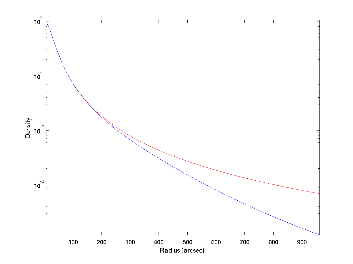
The SVM simplifies to a $\beta$-model when $\varepsilon=0$. Figure 5 shows the standard $\beta$-model (red) and SVM (blue) using $\varepsilon=5$, the steepest outer slope V06 allowed in their density fits. Here, we chose typical parameters, found in cluster fits, for the components common to the two profiles (namely, we chose $r_{c}=100\arcsec$ and $\beta=0.7$, and set the normalization $\rho_{0}=1$ for simplicity). For the SVM, we chose a scale radius of $r_{s}=500\arcsec$, corresponding to the radius at which the density of a typical cluster at low redshift begins to steepen. Note that since X-ray surface brightness scales as $\rho_{\rm gas}^{2}$, the signal will be $<0.1\%$ that of the core for the regions where the profiles diverge ($r>200\arcsec$).

5 Combining the N07 and SVM Profiles

We apply the N07 pressure profile (Eq. 17) to fit the SZA data presented in Chapter 5, combining it with the SVM (Eq. 18) to fit complementary Chandra X-ray imaging data. As discussed in §4, fitting X-ray surface brightness (Eq. 8) requires both density and temperature information. Having assumed the ideal gas law (Eq. 10), the electron temperature profile $T_{e}(r)$ occupies a unique position while jointly fitting the N07+SVM profiles to X-ray+SZE cluster observations: it can be derived from the pressure and density fits without relying on X-ray spectroscopy. For each iteration of the MCMC fitting routine, the temperature profile necessary to fit the X-ray surface brightness is derived for each set of test parameters of the density and pressure profiles. The weak temperature dependence of the X-ray imaging data (discussed in §4) has the ability to exclude some of the pressure model’s parameters that fit well the SZE data alone, as will be shown in Chapter 5.

4 Markov chain Monte Carlo Analysis

A Markov chain Monte Carlo (MCMC) method, implemented in a program called markov, is used to determine the distribution of models that fit the data, as described by Bonamente et al. (2004); LaRoque et al. (2006); Bonamente et al. (2006, 2008). Iterations are accepted in the MCMC according to the Metropolis-Hastings algorithm, which ensures that a fully-converged MCMC reflects the true probability distribution of the resulting model fits. Assuming the model itself as a prior, the output chain of parameters – the “Markov chain” itself – can be used to determine the probability density of the model fits.

The SVM has five free parameters to describe the gas density (see Eq. 18), and the N07 profile has two free parameters to describe the electron pressure (see Eq. 17). Additional parameters such as the cluster centroid, the X-ray background level, and the positions, fluxes, and spectral indices of field radio point sources are also included as necessary.

The model fitting code was originally called jointfit, and used a downhill simplex method (see, for example, Bonamente et al. 2004; Joy et al. 2001; Grego et al. 2000, 2001; LaRoque et al. 2003; Patel et al. 2000; Reese et al. 2000, 2002, and references therein). markov and jointfit have been used extensively to fit Chandra and ROSAT X-ray observations jointly with SZE observations made by OVRO and BIMA. Because the UVFITS files produced from SZA data contain sixteen bands, as opposed to the single-banded UVFITS files from OVRO/BIMA, markov’s UVFITS reader required an upgrade in order to read and properly account for the frequency of each band. Furthermore, in the transition from 32-bit to 64-bit desktop processors, the standard CFITSIO libraries did not work, and I upgraded the reader to the well-documented UVFITS reader Martin Shepherd wrote for Difmap (Shepherd 1997).

For each iteration in the MCMC process, model test parameters are generated by stepping randomly from the last accepted link in the Markov chain. The size of the step is determined using a top hat distribution of adjustable width. These test parameters are used to compute the model image over a regular grid, with sampling defined to be less than half the smallest scale the SZA can probe (i.e. Nyquist sampling of the scale probed by the longest baseline in the observation). This image is multiplied by the primary beam of the SZA, transformed via FFT to Fourier space (which is where the data are directly sampled by a radio interferometer), and interpolated to the Fourier-space coordinates of the SZE data. The likelihood calculation for the SZE data is then performed directly in Fourier space, where the noise properties of the interferometric data are well-characterized.

The MCMC routine determines which trial sets of parameters are accepted into the Markov chain by computing the joint likelihood $\mathcal{L}$ of the models’ fits to the X-ray and SZE data. The SZE likelihood is given by

$$\ln(\mathcal{L}_{\text{SZE}})=\displaystyle\sum_{i}\left[-\frac{1}{2}\left(\Delta R_{i}^{2}+\Delta I_{i}^{2}\right)\right]W_{i}$$ (19)

where $\Delta R_{i}$ and $\Delta I_{i}$ are the difference between model and data for the real and imaginary components at each point $i$ in the Fourier plane, and $W_{i}$ is a measure of the Gaussian noise ($1/\sigma^{2}$). Since the X-ray counts, treated in image space, are distributed according to Poisson statistics, the likelihood of the surface brightness model fit is given by

$$\ln(\mathcal{L}_{\text{Xray}})=\displaystyle\sum_{i}\left[D_{i}\ln(M_{i})-M_{i}-\ln(D_{i}!)\right]$$ (20)

where $M_{i}$ is the model prediction (including cluster and background components), and $D_{i}$ is the number of counts detected in pixel $i$. Spatial regions of the X-ray image, containing for example the cluster core, gas clumps, or X-ray point sources, can be excluded from the X-ray analysis simply by excluding data in those regions from the X-ray likelihood calculation (Eq. 20).

The joint likelihood of the X-ray and SZE models is given by $\mathcal{L}=\mathcal{L}_{\text{SZE}}\cdot\mathcal{L}_{\text{Xray}}$. For the models that include X-ray spectroscopic temperature constraints, the likelihood is $\mathcal{L}=\mathcal{L}_{\text{SZE}}\cdot\mathcal{L}_{\text{Xray}}\cdot\mathcal{L}_{\text{XSPEC}}$, where $\mathcal{L}_{\text{XSPEC}}$ comes from a table of $\chi^{2}$ values computed using a plasma emissivity model fit to the X-ray spectroscopic data, using the software package XSPEC (Arnaud 1996). The relationship between $\chi^{2}$ and $\mathcal{L}_{\text{XSPEC}}$ is

$$\mathcal{L}_{\text{XSPEC}}=\exp\left(-\frac{\chi^{2}}{2}\right).$$ (21)

Throughout a markov run, the probability distribution of fits to the data is explored. Some number of iterations at the beginning of the Markov chain, however, will depend on the starting parameters markov chooses; We refer to this as the “burn-in period” – when the MCMC still depends on the starting conditions – and ignore iterations accepted during this period. After a sufficiently large number of total iterations, the allowed range of parameters is fully explored. The number of required iterations depends on the number of free parameters, the size of the top-hat distribution out of which the test parameters are chosen, and the noise in the data. This is why we use convergence tests, described below, to determine the total number of required iterations.

The likeliest parameters will appear multiple times in the Markov chain. Their distribution after the initial burn-in period is referred to as the “stationary distribution,” since further iterations do not yield better constraints on the model. We follow the methods outlined in Bonamente et al. (2004), first exploring large regions of parameter space with test runs to ensure the solution is not stuck in a local minimum. Further runs are used to narrow in on the likeliest parameters by limiting the parameter range to explore and tuning the top hat distribution width. As in Bonamente et al. (2004), we use the Raftery-Lewis test to determine convergence to a stationary distribution (Raftery & Lewis 1992; Best et al. 1995; Gilks et al. 1996; Plummer et al. 2006), This is an efficient way to determine how many iterations the initial burn-in should contain, and how many further iterations are required to reach the stationary distribution. Once the MCMC routine has found the stationary distribution, we use the set of accepted model parameters to derive cluster parameters such as $M_{\mbox{\scriptsize tot}}$ and their error bars.

5 Mass analysis

1 Weighting factors for the cluster gas

The first quantity we consider is the cluster gas density. X-ray spectroscopic data have the ability to constrain the metallicity $Z$ of a gas (the mass fraction of elements heavier than helium) by fixing the abundance ratios to those observed in the solar atmosphere and fitting for the few prominent emission lines –notably those from iron – that can be found in X-ray spectra. Since the lighter elements (e.g. hydrogen, helium) are fully collisionally-ionized at cluster temperatures ($\gtrsim 1{\rm keV}$), no emission lines are observed from these, and their abundances are assumed to be those produced by Big Bang Nucleosynthesis (a.k.a. “cosmic abundance”), plus the amount produced by stellar nucleosynthesis, for the X-ray spectral fit to the metals.

When comparing the SZE-derived temperature (see § 5) to the X-ray spectroscopic temperature, we use the program XSPEC (Arnaud 1996) to fit a plasma emissivity model to the X-ray data. The plasma spectroscopic emission models we most commonly fit to these data are the Raymond-Smith (Raymond & Smith 1977) and MEKAL (Mewe et al. 1985; Kaastra & Mewe 1993; Liedahl et al. 1995) models, which can have free parameters of temperature, redshift, and metallicity (redshift is often fixed to that found using complementary optical observations, though typical X-ray data can constrain a cluster’s redshift to better than $\pm 1\%$). Fitting simulated cluster emission with X-ray spectra generated using the MEKAL model, we found that the metallicity recovered in XSPEC from fits of the Raymond-Smith model was within $\gtrsim 80\%$ accuracy of the metallicity in the input MEKAL spectrum.

Using the fit metallicity, we tested the X-ray surface brightness fitting procedure – which relies on the Raymond-Smith model when fitting X-ray emissivity – against mock X-ray observations of these simulated clusters. While these mock X-ray exposures were generated using the MEKAL model, the emissivity $\Lambda_{ee}(T_{e},Z)$ used to fit the mock observations (in Eq. 8) was computed using the Raymond-Smith model. The recovered gas density was accurate to better than 98%. We conclude that the continuum emission in an X-ray image is insensitive to the plasma emissivity model assumed in the fit, and continue to use the Raymond-Smith model to fit X-ray surface brightness.

Element Mass Fraction Number of Species Mass H $X=n_{\rm H}/(n_{\rm H}+4n_{\rm He})$ $1e^{-}+1p^{+}$ $1m_{p}$ He $Y=4n_{\rm He}/(n_{\rm H}+4n_{\rm He})$ $2e^{-}+1\alpha^{2+}$ $4m_{p}$

Table 1: Common parameters used to compute the weighting factors for a pure H and He plasma.

After determining the metallicity of the ICM (for either real or mock observations), several useful “weighting factors” can be determined by carefully accounting for the species of which the gas is composed. The weight per particle $\mu$ is determined by summing the masses of all the species (i.e. the electrons, protons, and atomic nuclei) in the plasma and dividing by one proton mass per particle.

$$\mu=\frac{n_{\rm H}\times 1m_{p}+n_{\rm He}\times 4m_{p}}{\left[n_{\rm H}(1e^{-}+1p^{+})+n_{\rm He}(1\alpha^{2+}+2e^{-})\right]m_{p}}.$$ (22)

For example, a fully-ionized plasma consisting of 10% helium and 90% hydrogen by number yields

$$\mu=\frac{0.9+0.1\times 4}{0.9(1e^{-}+1p^{+})+0.1(1\alpha^{2+}+2e^{-})}=0.62,$$ (23)

where we use the nomenclature $e^{-}$ for an electron, $p^{+}$ for a proton, and $\alpha^{2+}$ for a helium nucleus, and we have assumed a hydrogen atom is exactly one proton mass $m_{p}$ and a helium atom is $4m_{p}$ (see Table 1).

Similarly, we can define $\mu_{e}$, the weight per electron, by summing the masses of the species and dividing by $1m_{p}$ for each electron.

$$\mu_{e}=\frac{n_{\rm H}\times 1m_{p}+n_{\rm He}\times 4m_{p}}{\left[n_{\rm H}(1e^{-})+n_{\rm He}(2e^{-})\right]m_{p}},$$ (24)

For the example in Eq. 23, this means

$$\mu_{e}=\frac{0.9+0.1\times 4}{0.9(1e^{-})+0.1(2e^{-})}=1.18,$$ (25)

In practice, the detailed calculation of weighting factors requires accounting for all the species in the gas. Having fit spectroscopically a metallicity $Z$, we use the abundance calculation of Anders & Grevesse (1989) to determine the relevant weighting factors. We assume this abundance model for all results presented in this thesis (though we consider the effects of a non-universal, non-constant $Y/X$ ratio in §6).

2 Relating the fit $n_{e}(r)$ and $P_{e}(r)$ to ICM gas properties

The quantities $\mu_{e}$ can now be used to relate the electron number density profile $n_{e}(r)$ to the gas (mass) density $\rho_{\rm gas}(r)$, which is

$$\rho_{\rm gas}(r)=\mu_{e}m_{p}n_{e}(r).$$ (26)

Similarly, the number density of all species in the gas $n(r)$ relates to the gas density through $\mu$:

$$\rho_{\rm gas}(r)=\mu m_{p}n(r).$$ (27)

Assuming the electron temperature equals the gas temperature ($T_{e}=T_{\rm gas}$), we combine Eqs. 26 & 27 and use the ideal gas law to find the electron pressure profile relates to the overall gas pressure via

$$P_{\rm gas}(r)=\left(\frac{\mu_{e}}{\mu}\right)P_{e}(r).$$ (28)

3 Mass of the X-ray-Emitting ICM Gas ($M_{\mbox{\scriptsize gas}}$)

For a spherically-symmetric density profile, we now simply integrate $\rho_{\rm gas}(r)$ to obtain the gas mass $M_{\mbox{\scriptsize gas}}$ within a spherical volume with radius $r$:

$$\mbox{$M_{\mbox{\scriptsize gas}}$}(r)=4\pi\int_{0}^{r}\!\rho_{\rm gas}(r^{\prime})r^{\prime 2}dr^{\prime}.$$ (29)

4 The Total Mass of the Cluster ($M_{\mbox{\scriptsize tot}}$)

The total gravitational mass within a spherically-symmetric system in pressure equilibrium can be found by considering the balance between the inward gravitational force $f_{in}$ and the outward pressure $f_{out}$. This scenario of pressure support and negligible net mass transport across the surface of the sphere is known as hydrostatic equilibrium (HSE).

Consider the forces on a spherical shell of thickness $dr$, at radius $r$, with gas mass $m=4\pi r^{2}\,\rho_{\rm gas}(r)\,dr$. The inward force of gravity is

$$f_{in}=-\frac{G\,m\,\mbox{$M_{\mbox{\scriptsize tot}}$}(r)}{r^{2}}=-\frac{G\,4\pi r^{2}\,\rho_{\rm gas}(r)\,\mbox{$M_{\mbox{\scriptsize tot}}$}(r)dr}{r^{2}}$$ (30)

where $G$ is Newton’s gravitational constant and $M_{\mbox{\scriptsize tot}}$(r) is the total gravitating mass within radius $r$. The outward force of pressure is

$$f_{out}=4\pi r^{2}\left(\frac{dP_{\rm gas}}{dr}\right)dr$$ (31)

Setting $f_{in}=f_{out}$ and solving for $M_{\mbox{\scriptsize tot}}$(r) yields

$$\mbox{$M_{\mbox{\scriptsize tot}}$}(r)=-\frac{r^{2}}{G\rho_{\rm gas}(r)}\left(\frac{dP_{\rm gas}}{dr}\right)$$ (32)

Notice that this is a powerful way of using the observable gas distribution in a cluster of galaxies to estimate its total matter content (i.e. dark + baryonic). By assuming further the pressure is entirely thermal and that the ideal gas law holds, one only has to determine two of the three quantities {$P_{\rm gas}(r)$, $\rho_{\rm gas}(r)$, and $T(r)$} in order to estimate a cluster’s total mass.

5 Hot Gas Mass Fraction ($f_{\mbox{\scriptsize gas}}$)

For each accepted iteration in the MCMC, we have a set of model parameters fit to the available SZE+X-ray data, from which we can compute $M_{\mbox{\scriptsize gas}}$ and $M_{\mbox{\scriptsize tot}}$. Solving for $M_{\mbox{\scriptsize gas}}$ and $M_{\mbox{\scriptsize tot}}$ using Eqs. 29 & 32, we simply solve for the profile of the gas mass fraction individually for each set of MCMC parameters:

$$\langle\mbox{$f_{\mbox{\scriptsize gas}}$}(r)\rangle=\langle\mbox{$M_{\mbox{\scriptsize gas}}$}(r)/\mbox{$M_{\mbox{\scriptsize tot}}$}(r)\rangle.$$ (33)

Doing this, the mean gas fractions we present in this thesis take advantage of the fact that MCMC explores the probability density of model fits to the data. Furthermore, the confidence intervals presented also directly reflect the range of models fit (rather than assuming the derived $M_{\mbox{\scriptsize gas}}$ and $M_{\mbox{\scriptsize tot}}$ are statistically independent).

6 Overdensity Radius

In order to compute global cluster properties such as $M_{\mbox{\scriptsize gas}}$, $M_{\mbox{\scriptsize tot}}$, and $f_{\mbox{\scriptsize gas}}$, one needs to define a radius out to which all quantities will be calculated. Following LaRoque et al. (2006); Bonamente et al. (2006), we compute global properties of clusters enclosed within the overdensity radius $r_{\Delta}$, within which the average density of the cluster is a specified fraction $\Delta$ of the critical density, via

$$\frac{4}{3}\pi\,\rho_{c}(z)\,\Delta\,r_{\Delta}^{3}=\mbox{$M_{\mbox{\scriptsize tot}}$}(r_{\Delta}),$$ (34)

where $\rho_{c}(z)$ is the critical density of the Universe at redshift $z$, and is computed (with respect to $\rho_{c}=3H_{0}^{2}/8\pi G$, the critical density at redshift $z=0$):

$$\rho_{c}(z)=\rho_{c}\,[\Omega_{M}(1+z)^{3}+\Omega_{\Lambda}].$$ (35)

Throughout this work, we evaluate cluster properties at density contrasts of $\Delta=2500$ and $\Delta=500$, corresponding to average densities of 2500 and 500 times the critical density at the redshift of the cluster. The overdensity radius $r_{2500}$ has often been used in previous SZE+X-ray studies, since that was the maximum radius attainable in many X-ray observations of intermediate redshift clusters (see, e.g. LaRoque et al. (2006)). The overdensity $r_{500}$ is now reachable in deep SZA and Chandra X-ray data, without extrapolating the model beyond the image fitting region or into regions with signal-to-noise ratio $S/N\lesssim 1$.

6 SZE-Specific Quantities

1 The Integrated, Intrinsic Compton $y$ Parameter ($Y_{\mbox{\scriptsize int}}$)

Since the SZE signal arises via Compton scattering, the integrated SZ effect, when scaled to the distance of the cluster, can be converted to $Y_{\mbox{\scriptsize int}}$, the intrinsic, integrated Compton $y$ parameter (see e.g. da Silva et al. (2004); Nagai (2006)). The intrinsic line-of-sight (abbreviated “los” in the subscripts to follow) integrated Compton $y$ parameter $Y_{\mbox{\scriptsize los}}$ is obtained by integrating $y$ (Eq. 2) over the solid angle $\Omega$ subtended by the cluster, and scaling the area for the angular diameter distance of the cluster,

$$\mbox{$Y_{\mbox{\scriptsize los}}$}\equiv{D_{A}^{2}}\int_{\Omega}y~{}d\Omega=\frac{\sigma_{T}}{m_{e}\,c^{2}}\int_{-\infty}^{\infty}\!\!d\ell\int_{A}\!P_{e}\,dA.\\$$ (36)

Here $A$ is the area of the cluster in the plane of the sky.

In addition, SZE observations constrain the intrinsic volumetric (abbreviated “vol” in the subscripts to follow) integrated Compton $y$ parameter $Y_{\mbox{\scriptsize vol}}$, obtained by integrating $y$ within a spherical volume of radius $r$:

$$\mbox{$Y_{\mbox{\scriptsize vol}}$}=\frac{4\pi\,\sigma_{T}}{m_{e}\,c^{2}}\int_{0}^{r}\!\!P_{e}(r^{\prime})\,r^{\prime 2}dr.\\$$ (37)

Since $Y_{\mbox{\scriptsize int}}$ – in the form of either $Y_{\mbox{\scriptsize vol}}$ and $Y_{\mbox{\scriptsize los}}$– scales as pressure (ergs/cm³) integrated over volume (cm³), it is proportional to the thermal energy content of the ICM within that volume. As the dominant form of kinetic energy in the ICM, thermal energy tracks the underlying gravitational potential, and ultimately the dark matter halo of the cluster, to the extent that HSE holds. SZE flux thereby provides a robust, low scatter proxy, $Y_{\mbox{\scriptsize int}}$, for total cluster mass, $M_{\mbox{\scriptsize tot}}$.

2 The Total Thermal Energy Content:
An SZE-only Scaling Quantity

A problem becomes apparent when one considers how the N07 pressure profile – or any profile fit to SZE data alone – could be used in an SZE survey to constrain cosmology. To maximize the utility of a cluster survey, it is crucial to understand how to relate a cluster’s observable properties to its total mass.

When using joint SZE+X-ray data, one has the luxury of solving for $M_{\mbox{\scriptsize tot}}$ by assuming HSE (Eq. 32). Joint SZE+X-ray fits therefore allow one to solve for $r_{\Delta}$, the radius that encloses matter overdensity $\Delta$. We can then compute $M_{\mbox{\scriptsize tot}}$$(r_{\Delta})$ and $Y_{\mbox{\scriptsize int}}$$(r_{\Delta})$ (e.g. either $Y_{\mbox{\scriptsize los}}$$(r_{\Delta})$ or $Y_{\mbox{\scriptsize vol}}$$(r_{\Delta})$, provided in Eqs. 36 & 37), which, for example, could be used to establish the $Y_{\mbox{\scriptsize int}}$$(r_{\Delta})$–$M_{\mbox{\scriptsize tot}}$$(r_{\Delta})$ scaling relation.

For an SZE-detected cluster with no complementary X-ray observation (or some independent estimate of $M_{\mbox{\scriptsize tot}}$, such as from lensing or galaxy velocity dispersion), the problem arises that we do not have a way to determine $r_{\Delta}$, and therefore do not know within which radius to compute $Y_{\mbox{\scriptsize int}}$$(r_{\Delta})$. There is no direct way to find $r_{\Delta}$ from an SZE-only observation of a cluster, since we do not know $\mbox{$M_{\mbox{\scriptsize tot}}$}(r)$ (see Eq. 34). Unlike the isothermal $\beta$-model, the N07 pressure profile can be integrated over an infinite volume, yielding a finite estimate for the total thermal energy content of the cluster. The thermal energy content should scale directly with the total mass of a cluster – to the extent that thermal pressure supports the cluster against gravitational collapse – and has been studied before by others (e.g. Afshordi et al. 2007). The total thermal energy content $E_{\text{tot}}$ of a cluster that can be described by the spherically-symmetric pressure profile $P_{\rm gas}(r)$ is

$$E_{\text{tot}}=\frac{3}{2}\int_{0}^{\infty}\!\!4\pi P_{\rm gas}(r)r^{2}dr.$$ (38)

Using Eq. 28, where the SZE-constrained electron pressure profile is parameterized in the form of the generalized NFW pressure profile (Eq. 14), a tool such as Mathematica^® can handily solve this integral. For $a\!>\!0$, $b\!>\!3$, and $c\!<\!3$, the integral converges, yielding

$$E_{\text{tot,genNFW}}=6\pi r_{p}^{3}\,P_{e,i}\,\left(\frac{\mu_{e}}{\mu}\right)\frac{\Gamma(\frac{b-3}{a})\,\Gamma(\frac{3-c}{a})}{a\,\Gamma(\frac{b-c}{a})}.$$ (39)

Here $\Gamma$ is the Euler gamma function. For fixed slopes $(a,b,c)$, the integral is only dependent upon profile parameters $P_{e,i}$ and $r_{p}$, and scales as $Y_{\mbox{\scriptsize vol}}$. The parameters recommended by Daisuke Nagai (personal communication) for his simulated clusters all had $a\in[0.5,2]$, $c\in[0.5,1.5]$, and $b\in[4,5]$, which covers a range consistent with a finite thermal energy content. The N07 profile provides $(a,b,c)=(1.3,4.3,0.7)$, which also yields finite thermal energy. In Figure 6, we show the N07 profile predicts a thermal energy content within a given radius that converges to a finite total value.

Figure 6: The ratio of the thermal energy content within a given radius to the total as $r\rightarrow\infty$, plotted for the fit to A1835 of the N07 pressure profile. The vertical line shows $r_{500}\simeq 360\arcsec\simeq 1.4~{}{\rm Mpc}$.

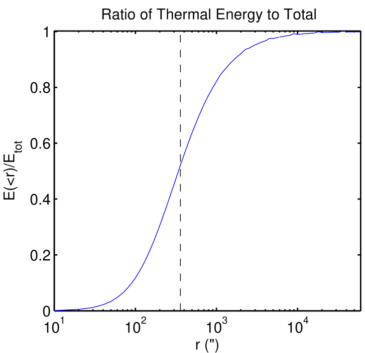
The fact that the integral for the ICM thermal energy (Eq. 38) converges implies there is a single, physical quantity that can be constrained by SZE data alone, without having to know $r_{\Delta}$ (which would otherwise have to be determined using independent, complementary observations). The total thermal energy is simply $\mbox{$Y_{\mbox{\scriptsize vol}}$}(r\rightarrow\infty)$ expressed in different units (c.f. Eqs. 37 and 38), and is not – by any means – a new concept. However, one could envision measuring how $E_{tot}$ scales with $\mbox{$M_{\mbox{\scriptsize tot}}$}(r_{500})$ for a small number of clusters that have high quality SZE and X-ray or lensing observations. Then, as a larger SZE survey (such as those planned for ACT and SPT) discovers new clusters through the SZE, this scaling relation could be directly applied to obtain an $\mbox{$M_{\mbox{\scriptsize tot}}$}(r_{500})$ estimate for each cluster in that sample, which is a useful step in constraining cosmology using clusters (see §1).

Comparison to the $\beta$-model for $E_{\text{tot}}$

In contrast to $E_{\text{tot,genNFW}}$, we note that the integral in Eq. 38 when applied to the $\beta$-model diverges for $\beta\leq 1$. For $\beta>1$, the total thermal energy of the cluster gas is

$$E_{\rm tot,\beta}=\frac{3}{2}\pi^{3/2}r_{c}^{3}\,P_{e,0}\,\left(\frac{\mu_{e}}{\mu}\right)\frac{\Gamma(\frac{3\beta-3}{2})}{\Gamma(\frac{3\beta}{2})}.$$ (40)

Since $\beta\approx 0.7$ for X-ray observations, the isothermal $\beta$-model generally predicts an infinite thermal energy content in clusters; this is a product of assuming isothermality where the assumption is no longer valid. As mentioned in §2, the generalized NFW profile can be simplified to the $\beta$-model by choosing $(a,b,c)=(2,3\beta,0)$. The condition that $\beta\!>\!1$ is required to obtain a finite total thermal energy within a cluster is consistent with the condition that the genNFW parameter $b\!>\!3$ (i.e. $\beta\!<\!1\Rightarrow b\!<\!3$).

Comparison of Total Thermal Energy to an X-ray Proxy

Recent work by Kravtsov et al. (2006) has demonstrated an X-ray quantity that, like the SZE quantity $Y_{\mbox{\scriptsize int}}$, provides a robust proxy for $M_{\mbox{\scriptsize tot}}$. This quantity is defined $Y_{X}\equiv\mbox{$M_{\mbox{\scriptsize gas}}$}(r_{500})\,T_{X}$. Here $T_{X}$ is measured within an annulus in radial range $[0.15,1]\,r_{500}$. This range was chosen because cluster temperature profiles are most self-similar over this range (Vikhlinin et al. 2005; Nagai et al. 2007b). This large core cut makes the measured $T_{X}$ insensitive to effects within cluster cores.

Using the ideal gas law (Eq. 10) and noting the similarity between the integral to obtain the gas mass $M_{\mbox{\scriptsize gas}}$ (Eq. 29) and that to obtain the thermal energy $E$ (Eq. 38), it is clear that $Y_{X}$ scales as the thermal energy content within $r_{500}$, assuming isothermality. The implication of this is that the SZE-determined thermal energy content could provide the basis for a powerful, SZE-only observable that could readily be applied to upcoming SZE cluster surveys, without the need for corroborating observations other than those required for redshift determination.

Chapter 5 Applications of the Models

In this chapter, I demonstrate the application of the N07+SVM (Eqs. 17 & 18) to observations of real clusters. I initially tested the markov fitting code and new models on mock SZA observations of several of the Kravtsov et al. (2005) simulated clusters. These mock SZA observations were also jointly fit with mock Chandra observations. The tests provided sufficient confidence that the modeling code was correctly implemented, but the mock SZA observations suffered systematic biases due to the unrealistically cuspy cores of these simulated clusters (see Fig. 3 and discussion in §1). Any attempt to excise these cluster cores, which often dominated the SZE signal, from the input simulation data would involve several assumptions about the cluster core and physics missing from the simulations. Instead I chose to use the mock observations to verify the functionality of the modeling code, and then focused on tests involving real observations of real clusters.

I selected three massive clusters, well studied at X-ray wavelengths, spanning a wide range of redshifts ($z$ = 0.17–0.89) and cluster morphologies. These clusters are used test the joint analysis of Chandra and SZA observations, using the models and methods described in Chapter 4. Specifically, I test the N07 pressure profile (Eq. 17) in conjunction with the SVM density profile (Eq. 18). I compare the results of these fits with results from a detailed, X-ray-only analysis, as well as with a joint SZE+X-ray analysis using the traditional isothermal $\beta$-model. I assume a $\Lambda$CDM cosmology throughout the analysis presented in this chapter, with $\Omega_{M}=0.3$, $\Omega_{\Lambda}=0.7$, and $\Omega_{k}=0$. The angular diameter distances to each of these clusters, as well as the redshifts and spectroscopic temperatures of the clusters, are listed in Table 1.

Cluster $z$ $d_{A}$ $T_{X}$ (Mpc) (keV) A1835 0.25  806.5 $9.95^{+0.36}_{-0.37}$ CL1226 0.89 1601.8 $9.62^{+1.69}_{-1.25}$ A1914 0.17  600.6 $8.63^{+0.47}_{-0.41}$

Table 1: Clusters chosen for testing the models. Angular diameter distances were computed assuming $\Omega_{M}=0.3$, $\Omega_{\Lambda}=0.7$, & $\Omega_{k}=0$.

Figure 1: X-ray image of A1835, showing it to be relaxed. The X-ray analysis of A1835 relies on a single Chandra ACIS-I exposure, with 85.7 ks of good time (unflagged exposure time). The pixels of the ACIS-I detector are binned to be 1.968on a side. The X-ray image shown here is smoothed with a Gaussian that is 2 pixels in width (for display purposes only). See Table 3 for more details on the X-ray observation. The inner 100 kpc (core) and all detected X-ray point sources were excluded from the X-ray surface brightness and spectroscopic analyses.

Figure 2: X-ray image of CL1226, showing this high redshift cluster to be approximately circular on the sky, and thus apparently relaxed. This image combines two Chandra exposures. The inner 100 kpc (core) and all detected X-ray point sources were excluded from the X-ray analysis.

Figure 3: X-ray image of A1914, showing it to be disturbed. This image combines two Chandra exposures. A large subclump, measured to be hot by M08, is located to the east (left) of the cluster center. This subclump, the inner 100 kpc (core), and all detected X-ray point sources were excluded from the X-ray analysis.

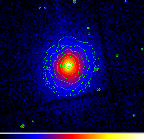
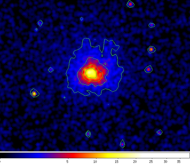
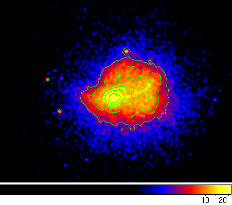
1 Cluster Sample

Abell 1835 (A1835) is an intermediate-redshift ($z=0.25$) cluster (see Fig. 1, located at the mean redshift of a sample of clusters being used by the SZA collaboration to determine the SZE flux scaling relations (versus $M_{\mbox{\scriptsize gas}}$, $M_{\mbox{\scriptsize tot}}$, $T_{X}$, etc.). This cluster sample is X-ray flux-limited, and is located in the redshift range $z\sim$ 0.2–0.3. The sample has both X-ray observations and optical lensing mass estimates available, and will appear in the thesis of Ryan Hennessey as well as forthcoming SZA papers. A1835 is relaxed, as evidenced by both its circular morphology in the X-ray images and its cool core (see Fig. 1, and Peterson et al. (2001) for more details). To demonstrate the applicability of the joint SZE+X-ray analysis to high redshift clusters, I analyzed CL J1226.9+3332 (CL1226), an apparently relaxed cluster at $z=0.89$ (see Maughan et al. (2007) – hereafter referred to as M07 –and Fig. 2). Note that M07 argues, despite appearing spherically symmetric, that the lack of a cool core in this cluster is likely due to a recent merger. Finally, to assess how applicable this pressure profile is to disturbed clusters, I also analyzed Abell 1914 (A1914), an intermediate redshift ($z=0.171$) cluster with a hot subclump near the core (see Fig. 3); when the subclump is not excluded from the X-ray analysis, a large centroid shift is present in the fit to the surface brightness (see Maughan et al. (2008) – hereafter referred to as M08 – who use the size of the error in the fit X-ray centroid as a measure of cluster dynamical state). I exclude this subclump from the X-ray analysis of A1914 by defining a $\sim 100$ kpc region centered on the peak brightness of the clump and excluding this region from the X-ray likelihood calculation (see Eq. 20 and discussion of the X-ray likelihood in §4).

Figures 4–7 show the clean-ed interferometric maps, produced from the SZA observations analyzed here, of these three clusters. Details of the SZA and Chandra observations, including the X-ray fitting regions, the unflagged, on-source integration times, and the pointing centers used for the SZE observations, are presented in Tables 2 and 3. Note that 90-GHz SZA data were included in the fits to CL1226, which is only partially resolved at 30 GHz due to its small angular extent (see §4).

Cluster SZA Pointing Center (J2000) Short Baselines (0.34–1.5 $\rm k\lambda$) Long Baselines (3–7.5 $\rm k\lambda$) $\rm{t_{int,red}}$ $\alpha$ $\delta$ beam($\arcsec\times\arcsec$) $\sigma$(mJy) beam($\arcsec\times\arcsec$) $\sigma$(mJy) (hrs) A1914 $14^{h}26^{m}00^{s}\!.8$ $+37^{\circ}49^{\prime}35\arcsec\!.7$ 117.5$\times$129.9 0.30 23.5$\times$17.4 0.35 11.5 A1835 $14^{h}01^{m}02^{s}\!.0$ $+02^{\circ}52^{\prime}41\arcsec\!.7$ 116.6$\times$152.1 0.25 17.5$\times$23.5 0.33 18.6 CL1226 (30 GHz) $12^{h}26^{m}58^{s}\!.0$ $+33^{\circ}32^{\prime}45\arcsec\!.0$ 117.4$\times$125.4 0.20 16.0$\times$21.2 0.20 22.0 CL1226 (90 GHz) “ ” “ ” 42.3$\times$39.1 0.42 9.74$\times$7.46 0.32 29.2

Table 2: SZA Cluster Observations

Cluster Joint SZE+X-ray Analysis Maughan X-ray Analysis ObsID (ks) (ks) A1914 26.0 34.4–423.1 23.3 0.0–462.5 542+3593 A1835 85.7 25.6–344.4 85.7 0.0–519.6 6880 CL1226 64.4 12.9–125.0 50 0.0–125.0 3180+5014 CL1226   N/A N/A 75+68 17.1–115 0200340101

Table 3: Details of X-ray Observations. The X-ray analysis presented here, as part of the joint SZE+X-ray modeling, was performed independently from that performed by Maughan.

In the following sections, I discuss the results of the joint analysis of the SZE and X-ray data. I show how the models fit the X-ray surface brightness and radio interferometric SZE data, and use these fits to place constraints on cluster astrophysical properties. Finally, I compare these results with an independent, detailed, X-ray-only analysis performed by Ben Maughan, following the techniques presented in M07 and M08 and described in §3. The high quality of the X-ray data on these three clusters allows this X-ray-only analysis, which is used in assessing the new models.

Figure 4: Cleaned SZA 30-GHz map of A1835, showing the detection to have a high significance of $\sim$ 22-$\sigma$ at the peak. This image, made with Difmap using only the short baseline data ($\sim$ 0.35–1.5 k$\lambda$), is for presentation purposes only; we fit our data directly in u,v-space, and do not use any interferometric mapping to determine cluster properties. Note that for a given u,v-space coverage, any unresolved structure in an interferometric SZE map of a cluster essentially “looks” like the synthesized beam; this determines the effective resultion of the observation. The synthesized beam is depicted in gray in the lower left corner. Contours are overlaid at 2-$\sigma$ intervals.

Figure 5: Cleaned SZA 30-GHz map of CL1226, showing the detection to have a significance of $\sim$ 10-$\sigma$ at the peak. See caption of Fig. 4 for further details.

Figure 6: Cleaned SZA 90-GHz map of CL1226, showing the detection with this higher resolution instrument to have a significance of $\sim$ 12-$\sigma$ at the peak. This observation was included since 30-GHz data alone could not constrain the radial profile of this high-redshift, small angular extent cluster (see Figures 10 and 11). See Fig. 4 for further details, noting the short baselines of the 90-GHz instrument are $\sim$ 1–4.5 k$\lambda$

Figure 7: Cleaned SZA 30-GHz map of A1914, showing the detection to have a high significance of $\sim$ 18-$\sigma$ at the peak. See Fig. 4 for detail.

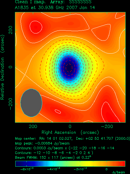
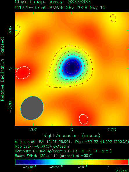
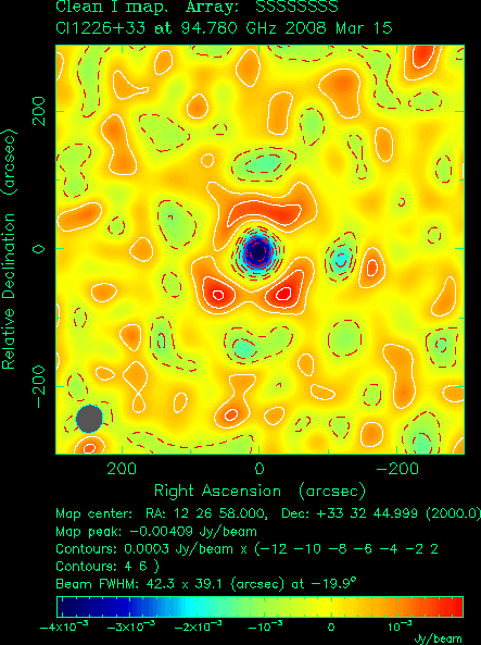
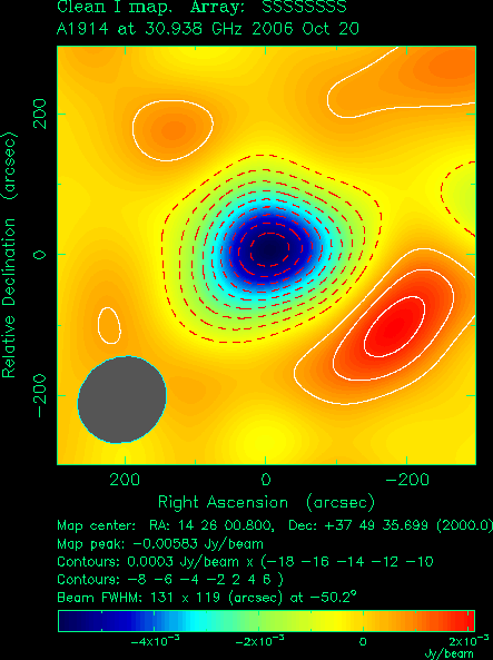
2 Unresolved Radio Sources

As discussed in §2, an unresolved, compact radio source (“point source”) can be represented mathematically by a 2-dimensional Dirac delta function in image space. In Fourier space, such unresolved sources – which can contaminate an SZE cluster observation – have an analytic transform: a constant, equal flux on all scales, as measured by all baselines. The flux from these sources is modeled analytically using a power law to describe the frequency-dependence of the source flux, with flux $f_{0}$ normalized at $\nu_{0}=30.938~{}\rm GHz$, the center of the SZA 30-GHz band. I also account for attenuation by the primary beam, $A_{\nu}(x,y)$, at each band’s frequency. Therefore, the measured flux $f(\nu)$ from a point source at map location $(x,y)$ is fit using

$$f(\nu)=A_{\nu}(x,y)f_{0}(\nu/\nu_{0})^{\alpha}$$ (1)

where $\alpha$ is the spectral index.

When modeling a compact source detected in an SZE observation, I fix its spectral index $\alpha$ so that it simultaneously fits the mean flux measured by the SZA at 30.938 GHz and that measured in the NVSS (Condon et al. 1998) or FIRST (White et al. 1997) surveys, which were performed at 1.4 GHz. The mean point source flux and the source’s approximate coordinates are first identified from the SZA observation(s) using the interferometric imaging package Difmap. This position serves as the input location in markov, which is then refined in trial markov runs. Such MCMC trials would sufficiently constrain the location of any newly-discovered point source, at least for the purposes of constraining point source contamination in an SZE observation. However, for all detected sources in the observations presented here, I found their trial positions agreed to within $\sim 2\arcsec$ of point sources already found by NVSS or FIRST. Since the VLA has superior resolution to the SZA, which constrains sources to within $\sim 7\arcsec$ positional uncertainty, I simply fixed each source’s location to the catalogued NVSS or FIRST position. I leave the source flux a free parameter in the Markov chains used to constrain cluster properties, so that the cluster SZE flux and any compact sources are simultaneously fit. This marginalizes over uncertainties in the SZE and point source fluxes.

In the SZA cluster observations presented here, the A1835 field contains two detectable compact sources at 30 GHz: a $2.8\pm 0.3$ mJy central source, and a $1.1\pm 0.3$ mJy source $\sim 1\arcmin$ from the cluster center (using the fixed position and spectral index for each source, as discussed above). The central source was detected in both the NVSS and the FIRST survey, while the weaker was only detected by FIRST. The SZA observation of CL1226 contains one detectable compact source, identified in both FIRST and NVSS, with a flux at 30 GHz of $4.0\pm 0.8$ mJy, located $\sim 6\arcmin$ from the cluster center (see also Muchovej et al. 2007). Flux from three compact sources, with positions constrained by NVSS and FIRST, was detected at 30 GHz in the A1914 field. The fluxes of the sources are $2.2\pm 0.3$ mJy, $1.3\pm 0.3$ mJy, and $0.6\pm 0.2$ mJy. The strongest was detected in both the NVSS and the FIRST survey, while the second strongest was only detected in the FIRST survey, and the weakest was only detected in NVSS. Figures 4–7 depict the SZA data with these point sources removed.

3 Independent X-ray Analysis

For each of these clusters, I compare the results of the joint SZE+X-ray analysis to the results of independent X-ray analyses, performed by Ben Maughan and described in detail in M07 and M08, which respectively presented the observations of CL1226 and A1914. The ACIS-I observation of A1835 used in this work became public more recently than M08 was published, and is therefore presented here – and in Mroczkowski et al. (2008) – for the first time. The observation of A1835 was calibrated and analyzed using the same methods and routines described in M08. Several key differences exist between both the M07/M08 data reduction and fitting methods, and those used in the joint SZE+X-ray analysis here (described in Bonamente et al. (2004, 2006), as well as in Appendix 7). I discuss a few salient differences here.

In the X-ray-only analysis, Maughan used blank-sky fields to estimate the background for both the imaging and spectral analysis. The X-ray images were binned into 1.97$\arcsec$ pixels (as are the images used in the joint SZE+X-ray analysis; see Appendix 7). The imaging analysis (primarily used to obtain the gas emissivity profile) is performed in the 0.7–2 keV energy band in order to maximize cluster signal to noise. Both the Chandra’s efficiency and the (redshifted) cluster emission are highest in this range (see Fig. 12); since spectral information is not preserved in the X-ray images used in the surface brightness fit, binning noisier photons from outside the 0.7–2 keV energy band can degrade the cluster signal, as the binning is unweighted (Appendix 7 discusses this further).

In Ben Maughan’s spectral analysis (used to derive both the global temperature $T_{X}$ and the temperature profiles), spectra extracted from each region of interest were fit in the 0.6–9 keV band with an absorbed, redshifted APEC (Smith et al. 2001) model. This absorption was fixed at the Galactic value. The global $T_{X}$, used in the isothermal $\beta$-model fits, is determined within an annulus with radius $r\in[0.15,1.0]\,r_{500}$.

An important consideration when using a blank-sky background method is that the count rate at soft energies can be significantly different in the blank-sky fields than the target field, due to differences between the level of the soft Galactic foreground emission in the target field and that in the blank-sky field. Ben Maughan accounted for this in the imaging analysis by normalizing the background image to the count rate in the target image in regions far from the cluster center. In his spectral analysis, this was modeled by an additional thermal component that was fit to a soft residual spectrum (the difference between spectra extracted in source free regions of the target and background datasets; see Vikhlinin et al. (2005)). The exception to this was the XMM-Newton data used in addition to the Chandra data for CL1226. A local background was found by M07 to be more reliable for the CL1226 spectral analysis, thus required no correction for the soft Galactic foreground.

The M07/M08 X-ray analysis methods exploit the full V06 density and temperature models (Eqs. 12 & 13) to fit the emissivity and temperature profiles of each cluster. The results of these fits are used to derive the total hydrostatic mass profiles of each system. Uncertainties for the independent, X-ray-only analysis are derived by Ben Maughan using a Monte Carlo randomization process. These fits involved typically $\sim$1000 realizations of the temperature and surface brightness profiles, fit to data randomized according to the measured noise. For further details about this fitting procedure, see M07 and M08.

4 SZE Cluster Visibility Fits

As mentioned in both §3 and §5, interferometric SZE data are in the form of visibilities, $V(u,v)$. Equation 7, which is an integral over all space ($\int\!\!\int\!dx\,dy$), relates the visibilities (in flux) to the spatial intensity pattern (in units of flux per solid angle on the sky, or flux density). Each visibility is thereby a measure of the flux within the Fourier mode probed by a given baseline.

Using relations provided in, e.g., Carlstrom et al. (2002), we can rescale the visibilities to a new quantity $Y(u,v)$, which is the integral of line-of-sight Compton $y$ within the Fourier modes probed by an interferometer. In the image plane, we can convert intensity to line-of-sight Compton $y$ using the CMB intensity $I_{0}$, the derivative of the blackbody function, and the spectrum of the SZE distortion $f(x)$ as a function of dimensionless frequency $x$ (Eq. 4). The derivative of the blackbody function multiplied by $f(x)$ yields the spectral dependence of the intensity shift in primary CMB due to the SZE, which is

$$g(x)=\frac{x^{4}e^{x}}{(e^{x}-1)^{2}}\left(x\frac{e^{x}+1}{e^{x}-1}-4\right).$$ (2)

The shift in primary CMB intensity due to the SZE, $\Delta I_{SZE}$, is

$$\Delta I_{SZE}=g(x)\,I_{0}\,y,$$ (3)

where the primary CMB intensity $I_{0}$ is

$$I_{0}=\frac{2(k_{B}\mbox{$T_{\mbox{\tiny CMB}}$})^{3}}{(hc)^{2}}.$$ (4)

Here $k_{B}$ is Boltzman’s constant, $T_{\mbox{\tiny CMB}}$ is the primary CMB temperature, $h$ is Planck’s constant, a nd $c$ is the speed of light.

Figure 8: Radially-averaged SZE model fits to A1835 in u,v-space, from the jointly-fit N07+SVM and isothermal $\beta$-model. The upper panels show the real (left) and imaginary (right) components of the visibilities, radially-averaged to be a function of $(u,v)$ radius, and rescaled to units of intrinsic, line-of-sight integrated Compton $y$; I plot here the frequency-independent quantity $Y(u,v)\,d_{A}^{2}=V(u,v)\,d_{A}^{2}/g(x)I_{0}$, where each band is scaled appropriately before binning, and the angular diameter distance is computed using the assumed $\Lambda$CDM cosmology. The lower panels show the reduced $\chi^{2}$ of the fits to the data for the chosen binning. The black points with error bars (1-$\sigma$) are the binned $Y(u,v)\,d_{A}^{2}$ data, with the point source models first subtracted from the cluster visibilities. The blue, solid line is a high likelihood N07 model fit, while the red, dashed line is a similarly-chosen fit of the $\beta$-model. For the available data points, both SZE models fit equally well (see lower panels, which shows the $\chi^{2}$ for each model is indistinguishable). However, note that as the u,v-radius approaches zero k$\lambda$ – where there are no data to constrain the models – the $\beta$-model predicts a much higher integrated Compton $y$ than the N07 model. For cluster data centered on the phase center of the observation (with both cluster and primary beam sharing this center), the mean imaginary component would equal zero. Since these model fits include the primary beam, which is not necessarily centered on the cluster, the small but non-zero imaginary component in the upper right panel is expected (note the smaller units for the $y$-axis of the right hand plot) (See, e.g. Reese et al. 2002, for comparison).

Figure 9: Radially-averaged SZE model fits for CL1226 in u,v-space. See Figure 8 for additional caption details. Note that the 30-GHz u,v-space coverage alone does not probe a sufficient range of cluster scales (see Figures 5 and 11) to determine where the SZE signal falls to zero. This results in poor constraints on the cluster’s radial profile when using 30-GHz data alone, and is a result of this high-redshift source being relatively compact on the sky (compared to A1835 and A1914; note that $r_{2500}$ is on the order of 1 arcminute, as shown in Table 4, §7). I therefore included 90-GHz SZA data (green) in the joint SZE+X-ray fit, since the 90-GHz instrument was designed to complement the u,v-coverage provided at 30-GHz (see Figures 10 & 11). Again, the small but non-zero imaginary component is expected, but note the smaller units for the plot of the imaginary component of the radially-binned $Y(u,v)$.

Figure 10: Radially-averaged SZE model fits for A1914 in u,v-space. See Figure 8 for details. Note that the slightly larger imaginary component in the upper right panel could be due to cluster asymmetry, since A1914 is disturbed and elliptical (see Fig. 7). Note that the reduced $\chi^{2}$ of this fit is no larger than those for the other two clusters (Figures 8 & 9).

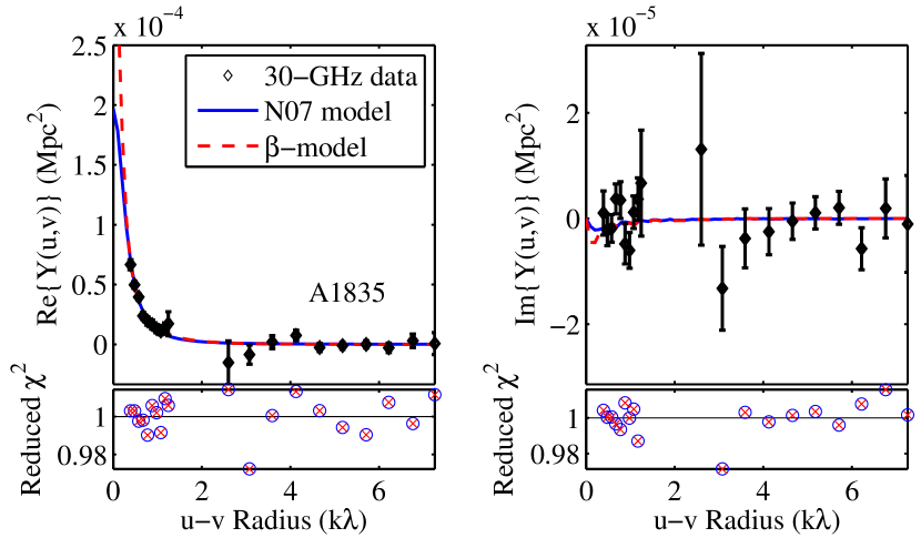
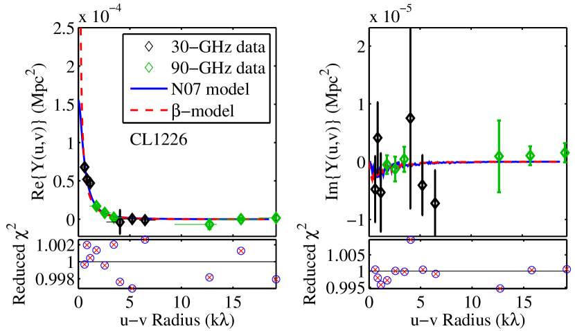
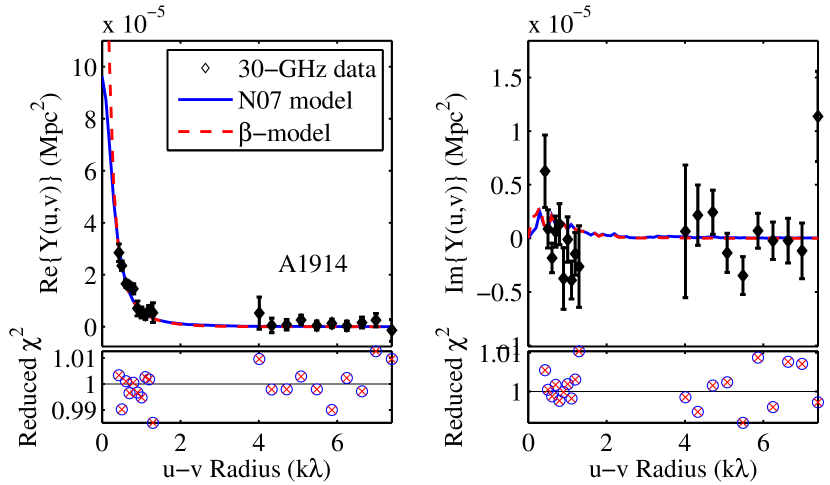
Figures 8–10 show representative, high-significance fits of the N07 and isothermal $\beta$-model to each cluster’s radially-averaged SZE visibility data (i.e. binned according to u,v distance). This quantity is then rescaled by $d_{A}^{2}/[g(x)I_{0}]$ to obtain the radially-averaged $Y(u,v)$ intrinsic to the cluster. This rescaling removes both the redshift and frequency dependence from the cluster visibility data, after having first subtracted all point source models (as modeled simultaneously with cluster in the MCMC fitting code) from the visibility data in u,v-space.

Note that for Figure 9, I combine both 30 and 90-GHz data to increase both the dynamic range and u,v-coverage on the high-redshift cluster CL1226. The u,v-coverage provided by the 30-GHz observation alone was insuffient to constrain the cluster’s profile. Figure 9 shows the 30-GHz data points at low u,v-radii agree to within their 1-$\sigma$ error bars, meaning the SZE signal from the cluster was not resolved by those baselines, nor does the 30-GHz data for CL1226 accurately determine where the signal falls to zero. The inclusion of 90-GHz data provides the necessary u,v-coverage and dynamic range to resolve the cluster profile. As detailed in §2, the 90-GHz instrument was designed to complement the u,v-coverage provided at 30-GHz (see Figures 10 & 11).

In Fig. 10, it can be seen that the average imaginary component of the radially-averaged $Y(u,v)$ of A1914 is slightly larger than that seen for the other two clusters (Figures 8 & 9). As mentioned in the caption, I attribute this to the disturbed, asymmetric nature of A1914, which is also apparent in the SZE image (see Fig. 7).

5 X-ray Surface Brightness Fits

The X-ray data reduction used in the joint SZE+X-ray analysis follows that from Bonamente et al. (2004, 2006), and is discussed in detail in Appendix 7. Each image was fit, excluding the inner 100 kpc from the X-ray imaging likelihood calculation (see §4), out to $\sim r_{500}$, using the Markov Chain Monte Carlo technique, described in §4, which jointly fits the X-ray and SZE data. Table 3 lists the precise fitting regions for each X-ray observation.

Figure 11: X-ray surface brightness profile fits to the clusters. The vertical dashed line denotes the 100 kpc core cut. The blue, solid line is the surface brightness computed using a high-likelihood fit of the N07+SVM profiles (analogous to the SZE fits plotted in Figures 8–10), while red, dot-dashed line is the surface brightness fit of a $\beta$-model. Both model lines include the X-ray background that was fit simultaneously with the cluster model (i.e. the plotted lines are the superpositions of each set of the background and cluster models, which were fit simultaneously to the X-ray imaging data). The black squares are the annularly-binned X-ray data, where the widths of the bins are denoted by horizontal bars. The vertical error bars are the 1-$\sigma$ errors on the binned measurements. Arrows indicate $r_{2500}$ and $r_{500}$ derived from the N07+SVM profiles (see §7).

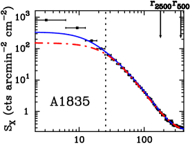
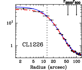
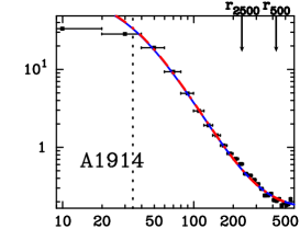
The surface brightness (Eq. 8) was modeled separately with both the isothermal $\beta$-model, using the spectroscopically-determined, global $T_{X}$ (measured within $r\in[0.15,1.0]\,r_{500}$), and the SVM, with temperature derived using the ideal gas law from the N07 pressure profile fit to the SZE data (as discussed in §5). Since the SVM was developed explicitly to be jointly fit with some form of the generalized NFW pressure profile, requiring both SZE and X-ray data, the X-ray surface brightness fit for the SVM contains information determined by the N07 pressure profile, which is primarily determined by SZE data. However, since X-ray surface brightness is a much stronger function of density than of temperature (Eq. 8), the SVM primarily determines the shape of the surface brightness fit.

Fig. 11 shows representative, high-likelihood (low $\chi^{2}$) fits to the surface brightness of each cluster, for both the SVM and isothermal $\beta$-model. For plotting purposes, the X-ray data are radially-averaged around the cluster centroid, which is determined by fitting the two-dimensional X-ray imaging data with the spherically-symmetric SVM and isothermal $\beta$-model profiles.

6 Fit Cluster Gas Profiles

The profiles parameterized in the models, which I apply in fitting the SZE visibilities and X-ray surface brightness data, are $P_{e}(r)$, $n_{e}(r)$, and $T_{e}(r)$. In this section, I discuss the recovered model fits of the parameters, and compare them with those fit in the detailed, independent X-ray analysis (§3). For the N07+SVM fits presented here, metallicity is fixed to the best-fit value determined from X-ray spectroscopic data.

Figure 12: $P_{e}(r)$ for each set of models fit to each cluster. The pressure from the jointly-fit N07+SVM is plotted in blue with vertical hatching. Pressure constrained by the SZE fit of the isothermal $\beta$-model is plotted using red, dot-dashed lines; note that the isothermal $\beta$-model’s shape is constrained by X-ray imaging data, and the only unique parameter to the SZE data in this fit is the central decrement (SZE normalization, see §1). Pressure derived from the density and temperature fits of the V06 profiles in the independent X-ray analysis is shown in black with grey shaded regions. See text in §6 for details. The vertical, black dashed line shows $r_{2500}$ derived from the N07+SVM fits, while the magenta dashed line is for $r_{500}$ (see Tables 4 and 5).

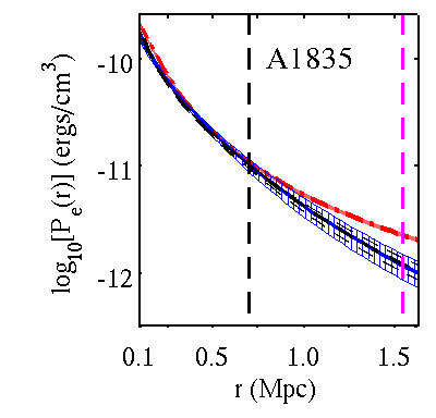
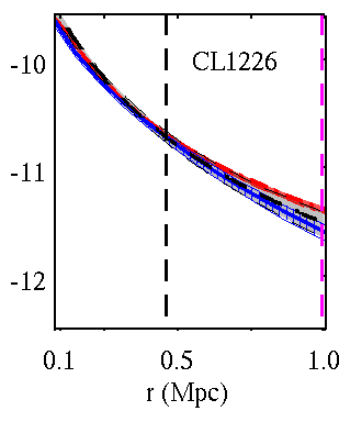
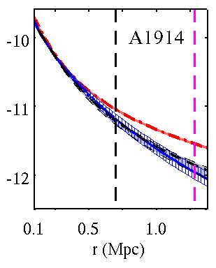
Figures 12–14 show the three-dimensional ICM radial profiles fit in the joint analysis of the SZA visibility + Chandra imaging data for A1835, CL1226, and A1914 (from left to right). In each figure, I compare the results, shown with their respective 68% confidence intervals, of each of the models and fitting procedures tested. The resulting constraints on $P_{e}(r)$, $n_{e}(r)$, and $T_{e}(r)$, using the MCMC routine to determine the probability density of each of the fits, are as follows:

• Pressure: Fig. 12 shows the pressure profile fit to the SZE data (blue for the N07 pressure profile fit jointly with the SVM profile to describe X-ray imaging), red for the isothermal $\beta$-model), and compares it with pressure derived from the V06 density and temperature profiles, which is constrained by the independent X-ray analysis (black), which utilizes X-ray spectroscopic information not used in the N07+SVM fitting. For all three clusters, the N07 pressure profile fits agree within their 68% confidence intervals with those predicted by the independent X-ray analysis.

  The pressure predicted by the isothermal $\beta$-model is in good agreement with the other model fits at $r\lesssim r_{2500}$, but is systematically higher in the cluster outskirts ($\gtrsim r_{2500}$). This is likely to be due to the fact that cluster temperature declines with radius (see Fig. 14), since the density estimates agree within $r\lesssim r_{500}$ (discussed in next subsection; see Fig. 13). Since the isothermal temperature $T_{X}$ is emission-weighted, the temperature is biased to favor the inner regions of a cluster (even when the core is excluded), where the density (and therefore the emission) is higher. The isothermal $\beta$-model predicts a large SZE signal in Fourier modes that are longer (lower u,v–radii) than the SZA interferometer can probe (see Figures 8–10). In contrast, the extra degree of freedom in the N07 model allows it to capture the true shape of the cluster’s pressure profile, since it fits pressure directly without relying on X-ray imaging to constrain the pressure profile’s shape. The X-ray imaging data are of much higher significance than the SZE visibility data, so they determine the shape of the isothermal $\beta$-model. In contrast, the parameters of the N07 model are only linked to the X-ray fit through the temperature derived from the N07+SVM profiles (see §5).

  

  

  

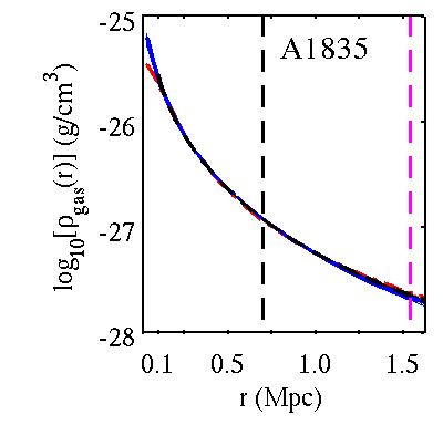
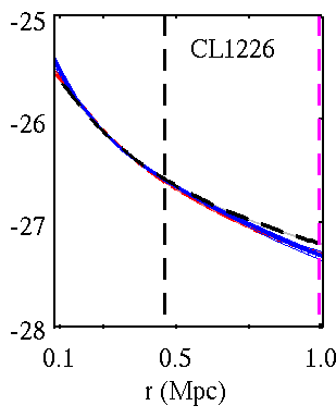
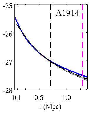
  Figure 13: $\rho_{\text{gas}}(r)$ for each set of models fit to each cluster. Colors and line styles are the same as in Fig 12. See text in §6 for details. Note that the vertical, black and magenta dashed lines show $r_{2500}$ and $r_{500}$, respectively, derived from the N07+SVM fits.

• Density: Fig. 13 shows the density fits to the X-ray imaging data from each cluster (where the SVM and isothermal $\beta$-model were jointly fit with the SZE data). Since the X-ray imaging data provide high significance measurements of $S_{X}$ (see Fig. 11), and since they are most sensitive to density (see Eq. 8), the X-ray data dominate the fit density. Since all three clusters have excellent X-ray data, density is tightly constrained for all three types of model fits. The additional flexibility in the SVM and V06 density profiles, which were built to fit departures from the $\beta$-model density profile in the cluster outskirts, were not necessary for any of these clusters.

  For all three clusters, the fits of the SVM density generally agree to within 1-2% of the full V06 density profile over the radial range $r\in[100~{}{\rm kpc},r_{2500}]$. Differences in the fit densities arise at larger radii, due to the differing X-ray background fitting procedures.

  The strong agreement between the densities derived from the SVM and the isothermal $\beta$-model at large radii is due to the fact that they use the same X-ray data and X-ray background levels, and none of the clusters had density profiles that diverged significantly from a $\beta$-model for the fitting regions considered here ($r\in[100~{}{\rm kpc},r_{500}]$). Note that the density fit from the isothermal $\beta$-model is overlaid in the plots by the SVM density fit (due to the strong agreement). This supports the argument the SZE data do not influence the shape parameters of the isothermal $\beta$-model ($r_{c}$ and $\beta$, Eq. 1).

  

  

  

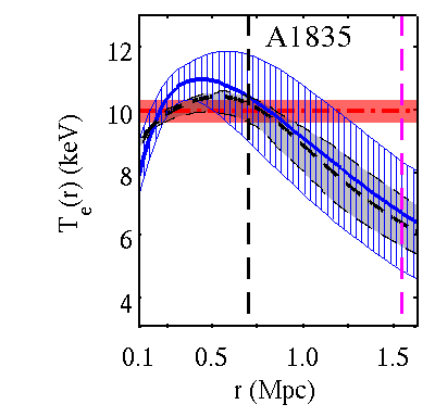
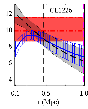
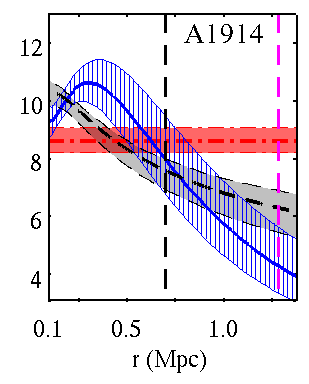
  Figure 14: $T_{e}(r)$ for each set of models fit to each cluster. Colors and line styles are the same as in Fig 12. Note that the isothermal $\beta$-model’s constant $T_{e}(r)=T_{X}$, constrained by the X-ray data, is plotted using red, dot-dashed lines and dark red shading. See text in §6 for details. Note that the vertical, black and magenta dashed lines show $r_{2500}$ and $r_{500}$, respectively, derived from the N07+SVM fits.

• Temperature: By not relying on X-ray spectroscopic temperature information when fitting the N07+SVM profiles to the SZE+X-ray data, $T_{e}(r)$ can be derived. This derived temperature profile provides a means by which we can diagnose how well the X-ray+SZE derived and X-ray spectroscopic temperatures independently agree. As shown in Fig. 14, the N07+SVM derived temperature profiles broadly agree with the V06 temperature profile fit to the X-ray spectroscopic data. For the relaxed cluster A1835, the median derived N07+SVM temperature profile is well within 1-$\sigma$ of the fit V06 $T_{e}(r)$ for nearly all radii outside the 100 kpc core. For CL1226, which is likely spherically-symmetric but has not had enough time to form a cool core (as argued in M07), the temperature agrees within 1-$\sigma$ at $r\in[r_{2500},r_{500}]$, but does not agree in the core.

  For the disturbed cluster A1914, the N07+SVM derived $T_{e}(r)$ agrees with Maughan’s fit $T_{e}(r)$ over a larger range than the isothermal $T_{X}$ does, but fails to capture the overall slope of $T_{e}(r)$. Since the N07 pressure profile was derived using relaxed clusters, it may not be surprising that the derived $T_{e}(r)$ could be biased; however, note that $P_{e}(r)$ does agree for the N07 and Maughan derived pressure (see Fig. 12), so the bias in the derived $T_{e}(r)$ could arise from the assumption of spherical symmetry being applied to the density profile (which in the X-ray image is clearly clumpy; see Fig. 3).

  The assumption of isothermality shows good agreement (typically within 1-$\sigma$) within $r<r_{2500}$ with Maughan’s fit of the V06 temperature profile. As expected, the isothermal $T_{X}$ does not agree with the more sophisticated analysis in the cluster outskirts ($r>r_{2500}$). This implies that isothermality is a relatively poor assumption at large radii, as the temperature universally declines at large radii in fits that have more degrees of freedom.

  The radial electron temperature profiles $T_{e}(r)$ derived from the N07+SVM joint-fit model (§5) reproduce the spectroscopically-determined $T_{e}(r)$ from deep Chandra observations of clusters quite well. This approach provides a unique and potentially powerful probe of $T_{e}(r)$ for high-redshift clusters, for which X-ray spectroscopic temperatures are difficult and often expensive to obtain.

7 Derived Cluster Properties

In Tables 4 and 5, I report the global properties of individual clusters derived from the N07+SVM model fits to the SZE+X-ray data. I calculate all quantities (following the methods outlined in §5 & 6) at overdensity radii $r_{2500}$ and $r_{500}$, and compare them to results from both the jointfit isothermal $\beta$-model analysis and to the Maughan X-ray-only analysis.

At both $r_{2500}$ and $r_{500}$, the measurements of $Y_{\mbox{\scriptsize los}}$ derived from the joint N07+SVM and the X-ray-only analysis are consistent at the 1-$\sigma$ level, for all three clusters. The isothermal $\beta$-model analysis, however, overestimates $Y_{\mbox{\scriptsize los}}$ by $\sim$ 20%–40% at $r_{2500}$, and by $\sim$ 30%–115% at $r_{500}$. This is due to the large contribution to $Y_{\mbox{\scriptsize los}}$ (at every projected radius) from the cluster outskirts, where the $\beta$-model significantly overestimates the pressure.

In contrast, the determinations of $Y_{\mbox{\scriptsize vol}}$ at $r_{2500}$ are generally consistent among the three analyses, except in the case of CL1226, due to the lower fit pressure. The excellent agreement at this radius between $Y_{\mbox{\scriptsize vol}}$ derived using fits of either the isothermal $\beta$-model or the N07 profile arises directly from the constraints on SZE flux provided by $Y(u,v)$ (see §4). At $r_{500}$, however, the median $Y_{\mbox{\scriptsize vol}}$ values from the isothermal $\beta$-model are $\sim$20%–60% higher than either the N07+SVM or M08 results, due to the fact that isothermality is a poor description of the cluster outskirts. With more data points probing cluster scales $\sim r_{2500}$, the good agreement between the isothermal $\beta$-model’s determination of $Y_{\mbox{\scriptsize vol}}$ and that from the N07+SVM fit is expected at $r_{2500}$. However, with the X-ray data determining the shape parameters of the $\beta$-model (in particular, the value of $\beta$ that can describe density is too shallow to describe pressure in the cluster outskirts), the over-constrained isothermal $\beta$-model fails to capture accurately $\mbox{$Y_{\mbox{\scriptsize vol}}$}(r_{500})$.

Cluster $\theta_{2500}$ $r_{2500}$ $Y_{\rm los}$ $Y_{\rm vol}$ $M_{\rm gas}$ $M_{\rm tot}$ $f_{\rm gas}$ Model fit () (Mpc) ($10^{-5}{\rm Mpc}^{2}$) ($10^{-5}{\rm Mpc}^{2}$) ($10^{13}{\rm M_{\odot}}$) ($10^{14}{\rm M_{\odot}}$) Abell 1835 N07+SVM 178${}^{+6.0}_{-5.7}$ 0.70${}^{+0.02}_{-0.02}$ 12.40${}^{+1.58}_{-1.28}$ 8.85${}^{+0.89}_{-0.79}$ 5.98${}^{+0.27}_{-0.26}$ 6.18${}^{+0.65}_{-0.57}$ 0.097${}^{+0.005}_{-0.005}$ Maughan (this work) 169${}^{+5.5}_{-8.0}$ 0.66${}^{+0.02}_{-0.03}$ 11.58${}^{+0.61}_{-0.67}$ 7.88${}^{+0.49}_{-0.72}$ 5.77${}^{+0.25}_{-0.35}$ 5.30${}^{+0.53}_{-0.72}$ 0.109${}^{+0.009}_{-0.006}$ isothermal $\beta$-model 159${}^{+3.0}_{-2.9}$ 0.62${}^{+0.01}_{-0.01}$ 13.85${}^{+0.72}_{-0.67}$ 7.94${}^{+0.43}_{-0.40}$ 4.96${}^{+0.13}_{-0.12}$ 4.38${}^{+0.25}_{-0.24}$ 0.113${}^{+0.004}_{-0.004}$ CL J1226+3332.9 N07+SVM 53.0${}^{+1.9}_{-2.0}$ 0.41${}^{+0.01}_{-0.02}$  5.45${}^{+0.53}_{-0.50}$ 3.55${}^{+0.37}_{-0.37}$ 2.92${}^{+0.14}_{-0.15}$ 2.71${}^{+0.30}_{-0.30}$ 0.108${}^{+0.008}_{-0.007}$ Maughan et al. (2007) 57.3${}^{+1.6}_{-1.5}$ 0.45${}^{+0.01}_{-0.01}$  7.57${}^{+0.33}_{-0.34}$ 5.04${}^{+0.31}_{-0.28}$ 3.25${}^{+0.14}_{-0.13}$ 3.41${}^{+0.30}_{-0.26}$ 0.095${}^{+0.004}_{-0.004}$ isothermal $\beta$-model 54.7${}^{+4.7}_{-4.4}$ 0.43${}^{+0.04}_{-0.03}$  7.37${}^{+1.15}_{-1.02}$ 4.25${}^{+0.73}_{-0.64}$ 2.97${}^{+0.34}_{-0.30}$ 2.98${}^{+0.83}_{-0.66}$ 0.100${}^{+0.016}_{-0.013}$ Abell 1914 N07+SVM 233${}^{+12.8}_{-10.4}$ 0.68${}^{+0.04}_{-0.03}$  8.71${}^{+1.52}_{-1.09}$ 6.66${}^{+1.03}_{-0.76}$ 4.83${}^{+0.33}_{-0.27}$ 5.28${}^{+0.91}_{-0.67}$ 0.092${}^{+0.008}_{-0.008}$ Maughan et al. (2008) 218${}^{+7.1~{}}_{-5.7~{}}$ 0.63${}^{+0.02}_{-0.02}$  7.87${}^{+0.56}_{-0.55}$ 5.69${}^{+0.37}_{-0.38}$ 4.64${}^{+0.17}_{-0.16}$ 4.31${}^{+0.43}_{-0.33}$ 0.107${}^{+0.005}_{-0.006}$ isothermal $\beta$-model 204${}^{+5.7~{}}_{-5.1~{}}$ 0.59${}^{+0.02}_{-0.01}$ 11.28${}^{+0.59}_{-0.56}$ 6.24${}^{+0.34}_{-0.32}$ 4.04${}^{+0.15}_{-0.14}$ 3.52${}^{+0.30}_{-0.26}$ 0.115${}^{+0.005}_{-0.005}$

Table 4: $Y_{\rm los}$, $Y_{\rm vol}$, $M_{\rm gas}$, $M_{\rm tot}$, and $f_{\rm gas}$ for each model, computed within each model’s estimate of $r_{2500}$.

Cluster $\theta_{500}$ $r_{500}$ $Y_{\rm los}$ $Y_{\rm vol}$ $M_{\rm gas}$ $M_{\rm tot}$ $f_{\rm gas}$ Model fit () (Mpc) ($10^{-5}{\rm Mpc}^{2}$) ($10^{-5}{\rm Mpc}^{2}$) ($10^{13}{\rm M_{\odot}}$) ($10^{14}{\rm M_{\odot}}$) Abell 1835 N07+SVM 365${}^{+32}_{-22}$ 1.42${}^{+0.13}_{-0.09}$ 20.87${}^{+4.66}_{-3.00}$ 17.79${}^{+3.72}_{-2.45}$ 13.66${}^{+1.29}_{-0.90}$ 10.68${}^{+3.11}_{-1.85}$ 0.128${}^{+0.017}_{-0.020}$ Maughan (this work) 363${}^{+17}_{-12}$ 1.42${}^{+0.07}_{-0.05}$ 21.37${}^{+2.45}_{-1.58}$ 17.41${}^{+1.61}_{-0.99}$ 13.94${}^{+0.64}_{-0.52}$ 10.68${}^{+1.54}_{-1.01}$ 0.133${}^{+0.009}_{-0.012}$ isothermal $\beta$-model 361${}^{+7~{}}_{-6~{}}$ 1.41${}^{+0.03}_{-0.03}$ 34.53${}^{+1.78}_{-1.68}$ 21.29${}^{+1.09}_{-1.02}$ 13.29${}^{+0.27}_{-0.27}$ 10.30${}^{+0.58}_{-0.54}$ 0.129${}^{+0.005}_{-0.005}$ CL J1226+3332.9 N07+SVM 125${}^{+12}_{-9}$ 0.97${}^{+0.09}_{-0.07}$ 11.6${}^{+1.9}_{-1.6}$  9.53${}^{+1.50}_{-1.25}$ 8.44${}^{+0.64}_{-0.57}$  7.17${}^{+2.22}_{-1.48}$ 0.118${}^{+0.021}_{-0.022}$ Maughan et al. (2007) 115${}^{+3~{}}_{-3~{}}$ 0.89${}^{+0.02}_{-0.02}$ 13.9${}^{+1.3}_{-1.1}$ 10.59${}^{+0.69}_{-0.68}$ 8.30${}^{+0.32}_{-0.36}$  5.49${}^{+0.46}_{-0.47}$ 0.151${}^{+0.008}_{-0.008}$ isothermal $\beta$-model 127${}^{+10}_{-10}$ 0.99${}^{+0.08}_{-0.08}$ 18.3${}^{+2.7}_{-2.3}$ 11.91${}^{+1.71}_{-1.51}$ 8.32${}^{+0.68}_{-0.60}$  7.49${}^{+1.93}_{-1.60}$ 0.111${}^{+0.020}_{-0.016}$ Abell 1914 N07+SVM 425${}^{+37}_{-27}$ 1.24${}^{+0.11}_{-0.08}$ 12.69${}^{+2.76}_{-1.87}$ 11.01${}^{+2.32}_{-1.58}$ 10.11${}^{+0.94}_{-0.67}$  6.38${}^{+1.83}_{-1.13}$ 0.159${}^{+0.021}_{-0.024}$ Maughan et al. (2008) 448${}^{+24}_{-21}$ 1.29${}^{+0.07}_{-0.06}$ 13.47${}^{+1.68}_{-1.77}$ 10.78${}^{+1.03}_{-1.09}$ 10.24${}^{+0.45}_{-0.57}$  7.49${}^{+1.29}_{-1.00}$ 0.138${}^{+0.015}_{-0.018}$ isothermal $\beta$-model 461${}^{+13}_{-11}$ 1.34${}^{+0.04}_{-0.03}$ 29.08${}^{+1.52}_{-1.44}$ 17.07${}^{+0.87}_{-0.84}$ 11.05${}^{+0.36}_{-0.33}$  8.14${}^{+0.69}_{-0.59}$ 0.136${}^{+0.007}_{-0.007}$

Table 5: $Y_{\rm los}$, $Y_{\rm vol}$, $M_{\rm gas}$, $M_{\rm tot}$, and $f_{\rm gas}$ for each model, computed within each model’s estimate of $r_{500}$.

Figure 15: $Y_{\mbox{\scriptsize los}}$ computed within $6^{\prime}$ ($\sim 1.4~{}\rm Mpc$, which is $\approx r_{500}$ for this cluster) for fits to SZA observation of A1835. The bold, black contours contain 68% and 95% of the accepted iterations to the jointly-fit Chandra + SZA data, while the thinner, blue contours are those for fits to SZA data alone. Note that the vertical, black and magenta dashed lines show $r_{2500}$ and $r_{500}$, respectively, derived from the N07+SVM fits.

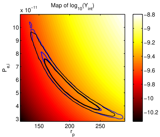
The N07 pressure profile (Eq. 17) – fit to SZE data alone or fit jointly to SZE+X-ray data – has just two free parameters to describe the SZE data: $P_{e,i}$ and $r_{p}$. In the joint fit N07+SVM, these parameters are only linked to the X-ray imaging data through the derived temperature (see discussion in §5). Figure 15 shows the degeneracy between $P_{e,i}$ and $r_{p}$ when fitting the SZA observations of A1835, comparing the SZE-only and the joint SZE+X-ray fits of the N07 profile. This degeneracy is similar to that between $r_{c}$ and $\beta$, when fitting the $\beta$-model to SZE data alone (see Grego et al. 2001, for example). These two quantities are not individually constrained by our SZE observations, but they are tightly correlated. The preferred region in the $P_{e,i}-r_{p}$ plane encloses approximately constant $Y_{\mbox{\scriptsize los}}$. As a result, the 68% confidence region allows less than $\pm$25% variation in $Y_{\mbox{\scriptsize los}}$, despite the much larger variation individually in $P_{e,i}$ and $r_{p}$. Since $Y_{\mbox{\scriptsize los}}$ at large radii scales with the cluster SZE flux probed by an interferometer (e.g. $Y(u,v)$ discussed in §4), this parameter is most directly constrained when fitting models to the SZE data.

The gas mass estimates – computed by integrating the gas density fit with either the jointly-fit SVM or the isothermal $\beta$-model (as discussed in §3) – agree with the gas mass estimates derived from the Maughan X-ray fits (Tables 4 and 5). This agreement is not surprising, given that the gas mass is determined in all cases from density fits to the X-ray surface brightness data. It demonstrates, however, that the 100 kpc core makes a negligible contribution to the total gas mass even at $r_{2500}$, and that excluding the core from the joint analysis does not therefore introduce any significant bias in our estimate of $M_{\mbox{\scriptsize gas}}$. Incidentally, it also shows that the additional components in the SVM and the full V06 density models were not necessary to fit these clusters.

Tables 4 and 5 also present estimates of the total masses, computed using each model’s estimate of the overdensity radius ($r_{\Delta}$, Eq. 34) for each Monte Carlo realization of the fit parameters. For two of the clusters, I find that the error bars are significantly larger for $M_{\mbox{\scriptsize tot}}$ determined from the N07+SVM fits than for the isothermal $\beta$-model or M08 fits. This is a consequence of the fact that the $\beta$-model analysis, with fewer free parameters and the assumption of isothermality, typically places strong but poorly-motivated priors on the total mass, while the M08 fits make use of the spatially resolved temperature profile afforded by the deep X-ray observations. CL1226 is the exception, with both the N07+SVM and M07 constraints on $M_{\mbox{\scriptsize tot}}$ being tighter than those provided by the isothermal $\beta$-model; the N07+SVM fits rely on high-significance SZE constraints provided by combining 30+90 GHz SZA data, while the M07 constraints are narrowed by using both XMM-Newton and Chandra spectroscopy. I find that the N07+SVM and M08 total mass estimates broadly agree at both $r_{2500}$ and $r_{500}$, leading to good overall agreement between gas fractions computed using the N07+SVM profiles and those from the Maughan X-ray fits. As discussed in §5, I compute the gas mass fraction $f_{\mbox{\scriptsize gas}}$ in a way that takes advantage of the fact that MCMC explores the probability density distribution of model fits to the data. Both the Maughan V06 and N07+SVM estimates of $f_{\mbox{\scriptsize gas}}$ within $r_{2500}$ are all consistent with the constant fraction found in Allen et al. (2004, 2007). The isothermal $\beta$-model, on the other hand, is too constrained to agree with the non-isothermal fits at both $r_{2500}$ and $r_{500}$; its estimate of $M_{\mbox{\scriptsize tot}}$ is moreover sensitive to the annulus within which $T_{X}$ is determined. This trend can also be seen in Figure 19, which shows $M_{\mbox{\scriptsize tot}}$$(r)$ for each cluster.

Figure 16: $y(R)$ – Compton $y$ (integrated along the line of sight, Eq. 2) as a function of sky radius $R$. Colors and line styles are the same as in Fig 12. See text in §6 for details. Note that the vertical, black and magenta dashed lines show $r_{2500}$ and $r_{500}$, respectively, derived from the N07+SVM fits.

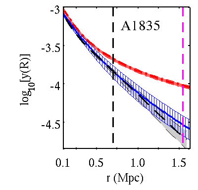
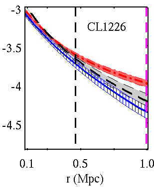
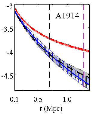
In addition to the data presented in Tables 4 and 5, which only show parameters computed at each model’s estimate of the overdensity radii $r_{2500}$ and $r_{500}$, I plot the derived cluster profiles and discuss them here:

• Compton $y$: Figure 16 shows $y(R)$ (integrated along the line of sight through the cluster, Eq. 2), for sky radius $R$, from the isothermal $\beta$-model and the N07 model, and compares it to $y(R)$ derived from Maughan’s fit density and temperature profiles. This quantity is simply the line-of-sight integral of electron pressure (see Eq. 2). It is worth noting that the excess pressure predicted by the $\beta$-model can translate to an over-prediction of $y(R)$ even at the cluster core. Because this excess is nearly constant over sky radius, it is not constrained by an interferometer, which is not sensitive to scales larger than a baseline probes (see discussion in §3). $y(R)$ from the N07 fits to A1835 and A1914 agrees well with that derived from the independent X-ray analysis, but disagrees to the extent that the N07 pressure drops off more rapidly for CL1226 than the X-ray-derived pressure. Simply put, the V06 density could be biased by assumptions about the X-ray background, leading to an overestimate of the density at large radii, which would contribute to the X-ray estimate of $y(R)$ (see discussion of the density fits in §6). While this may be disconcerting, the reader should note this is one of the drawbacks when using quantities integrated along an infinite sight line through the cluster; if the profile does not decline rapidly enough, the overestimate at large radii yields a non-negligible contribution.

  

  

  

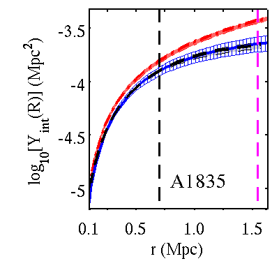
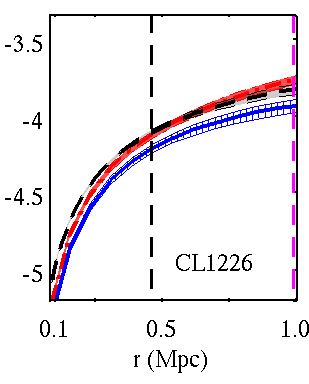
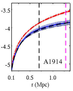
  Figure 17: $Y_{\mbox{\scriptsize los}}$ – Compton $y$ integrated over sky radius $R$. Colors and line styles are the same as in Fig 12. See text in §6 for details. Note that the vertical, black and magenta dashed lines show $r_{2500}$ and $r_{500}$, respectively, derived from the N07+SVM fits.

• $Y_{\mbox{\scriptsize los}}$ – the line-of-sight Integrated Compton $y$, integrated over an area of the sky: Figure 17 shows the SZE scaling quantity $Y_{\mbox{\scriptsize los}}$  integrated along the line of sight through the cluster and within a region of the sky (see §1, Eq. 36). Given the isothermal $\beta$-model’s $y(R)$, and the fact that the integral for $Y_{\mbox{\scriptsize los}}$ diverges for $\beta<1$, it is unsurprising that there is a large systematic difference, at large radii, between the models’ estimates. For A1835 and A1914, the estimates of $\mbox{$Y_{\mbox{\scriptsize los}}$}(R)$ from the SVM+N07 fits agree with those calculated from Maughan’s fits, which is expected given the agreement in $y(R)$.

  

  

  

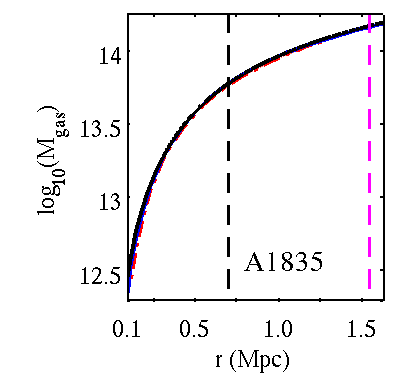
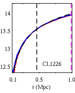
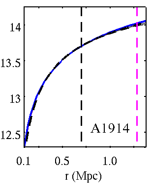
  Figure 18: $M_{\mbox{\scriptsize gas}}$ – the gas mass integrated within a spherical volume defined by cluster radius $r$. Colors and line styles are the same as in Fig 12. See text in §6 for details.

• $M_{\mbox{\scriptsize gas}}$– Gas Mass: Figure 18 shows the gas mass obtained by integrating the gas density within a spherical volume (using Eq. 29). Since the densities obtained using each method of fitting were similar (see Fig. 13), $M_{\mbox{\scriptsize gas}}$(r) obtained from each method is also similar. Note, however, that the independent X-ray analysis also modeled the cluster core, which contributes negligibly to the overall gas mass at large radii (such as $r_{2500}$ and $r_{500}$).

  

  

  

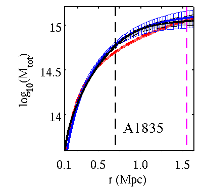
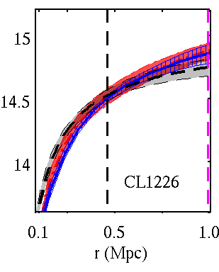
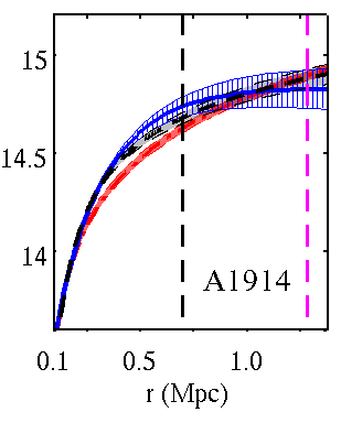
  Figure 19: $M_{\mbox{\scriptsize tot}}$ – the total mass estimated assuming hydrostatic equilibrium at cluster radius $r$. Colors and line styles are the same as in Fig 12. See text in §6 for details.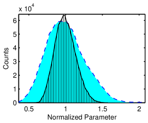

  

  Figure 20: 1-D histograms of the N07+SVM jointfit estimates, for A1835, of $M_{\mbox{\scriptsize tot}}$ and $Y_{\mbox{\scriptsize los}}$  normalized by their respective median values, $M_{\mbox{\scriptsize tot}}$is the cyan region with a dashed outline, and $Y_{\mbox{\scriptsize los}}$ is the vertically hatched region with a solid black outline. Both $M_{\mbox{\scriptsize tot}}$ and $Y_{\mbox{\scriptsize los}}$ are computed within a fixed radius of $\theta=360\arcsec$. The derived $Y_{\mbox{\scriptsize los}}$, which scales with integrated SZE flux, has a more tightly constrained and centrally peaked distribution than that of $M_{\mbox{\scriptsize tot}}$, as $M_{\mbox{\scriptsize tot}}$ is sensitive to the change in slope of the pressure profile (see Eqs. 16 & 32). Since the N07 model was developed primarily to recover $Y_{\mbox{\scriptsize int}}$ from SZE observations, it is useful to note how well this model performs in this capacity.

• $M_{\mbox{\scriptsize tot}}$– Total Mass: Figure 19 shows the total mass profile estimated by applying hydrostatic equilibrium to each model (Eq. 32). The total mass from the N07+SVM agrees with that from the independent X-ray analysis for most cluster radii, for all three clusters. In contrast, the isothermal $\beta$-model disagrees for A1835 and A1914 over a large range. Due to the steepness of the derived N07+SVM temperature profile of A1914 (see Fig. 14), its estimate of $M_{\mbox{\scriptsize tot}}$ flattens before $r_{500}$.

  Since the density fits are all well-constrained (see Fig. 13), the error bars from the isothermal $\beta$-model and the V06 fits performed by Ben Maughan arise almost entirely from the temperature constraints (including constraints on the derivative of temperature), while the error bars on $M_{\mbox{\scriptsize tot}}$ from the N07+SVM fits arise from those on the pressure profile and its derivative. Fig. 20 shows a comparison of the ability of the N07+SVM, when fit to X-ray imaging and SZE data, to constrain $M_{\mbox{\scriptsize tot}}$ and $Y_{\mbox{\scriptsize los}}$. The sparsely sampled u,v-data provide poorer constraints on $dP/dr$ than they do on $Y_{\mbox{\scriptsize los}}$, which scales with SZE flux. The relatively poor constraints on $dP/dr$ translate directly to error bars on $M_{\mbox{\scriptsize tot}}$.

  Unlike the N07+SVM, the isothermal $\beta$-model lacks the flexibility (by definition) to model a gas temperature profile that varies over the cluster’s radius. In Fig. 19, one can see that the total mass estimate from the isothermal $\beta$-mode never agrees with the independent, detailed X-ray-only analysis at both $r_{2500}$ and $r_{500}$. Where the isothermal $\beta$-model does agree depends mainly on the region within which $T_{X}$ was measured. Since the HSE estimate of $M_{\mbox{\scriptsize tot}}$ depends on the slope of the pressure profile (as discussed in §32), the fact that the isothermal $\beta$-model assumes a constant temperature ($dT/dr=0$), but recovers density well (e.g. Fig. 13), indicates the isothermal $\beta$-model will provide a systematically-biased estimate of $M_{\mbox{\scriptsize tot}}$ at some radii.

  

  

  

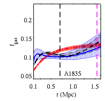
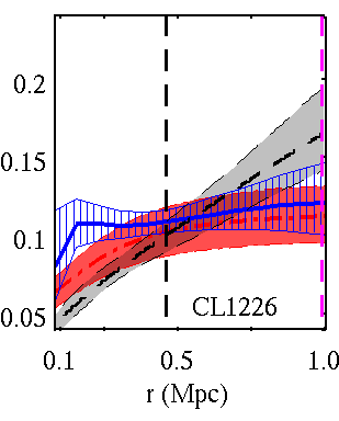
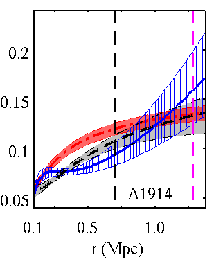
  Figure 21: $f_{\mbox{\scriptsize gas}}$ – the gas mass fraction, computed as $\mbox{$M_{\mbox{\scriptsize gas}}$}/\mbox{$M_{\mbox{\scriptsize tot}}$}$ at cluster radius $r$ for each accepted iteration in the Markov chain. Colors and line styles are the same as in Fig 12. See text in §6 for details.

• $f_{\mbox{\scriptsize gas}}$ – Hot Gas Fraction: Figure 21 shows the gas fraction, computed using each accepted MCMC iteration’s prediction for $M_{\mbox{\scriptsize gas}}$ and $M_{\mbox{\scriptsize tot}}$(as discussed in §5). The N07+SVM estimates of $f_{\mbox{\scriptsize gas}}$ at intermediate radii ($r\sim r_{2500}$) are consistent with previous, X-ray-only results (such as Allen et al. 2004, 2007). The flatness of the $M_{\mbox{\scriptsize tot}}$ profile derived from N07+SVM fits to A1914 leads to the prediction that $f_{\mbox{\scriptsize gas}}$${}_{,500}>\Omega_{b}/\Omega_{M}\approx 0.165$ (Hinshaw et al. 2008, assuming $h=0.7$), which seems unlikely. This suggests that the N07+SVM estimate of $M_{\mbox{\scriptsize tot}}$ for A1914 is too low at $r\sim r_{500}$, due to the steeply declining temperature profile discussed above.

8 Conclusions

I have applied a new model for the ICM pressure profile – motivated both by theory and detailed cluster observations – to fit the SZE signal from three galaxy clusters. I have also developed and tested a complementary density model – a simple extension to the $\beta$-model – that can be used jointly with this new SZE model to fit X-ray observations. I show the new pressure profile accurately captures the bulk properties of relaxed clusters outside the core, and out to $r_{500}$.

I also argue that this new model should supplant the isothermal $\beta$-model when attempting to use SZE data – interferometric or otherwise – to determine cluster SZE scaling relations. The additional degree of freedom, versus the isothermal $\beta$-model, in the N07 pressure profile allows it to more accurately describe a cluster that has been only sparsely sampled in u,v-space.

Finally, the derived temperature from the N07+SVM could prove to be a useful tool, either in independently confirming X-ray spectroscopic temperature measurements, or in measuring the temperatures of high-redshift clusters for which sufficiently deep X-ray exposures are unavailable, and are difficult to obtain. I present in Chapter 6 a way in which X-ray spectroscopic data can be used to provide additional constrains in the context of the N07+SVM profile.

Chapter 6 Extensions to the models

Throughout the cluster analysis presented in Chapter 5, I tested the new pressure and density models by discarding all X-ray spectroscopic temperature information from the joint SZE+X-ray fit, and using this information as an independent test. I used the SZE constraints on pressure to derive temperature, assuming the ideal gas law and a fixed $\Lambda$CDM cosmology with $\Omega_{\rm M}=0.3$, $\Omega_{\Lambda}=0.7$, $\Omega_{\rm k}=0$. In this section, I consider what additional tests can be performed by including spectroscopic temperature information.

For these proposed tests, we will choose a sample of relaxed clusters comprising many of the $\delta>-10^{\circ}$ clusters with publicly-available Chandra observations. By selecting apparently relaxed clusters, the impact of assuming spherical symmetry can be reduced.

1 Using X-ray Spectroscopic Data

Medium exposure observations of high redshift clusters typically provide too few photons to constrain their temperature profiles in detail. The most robustly-determined spectroscopic temperature for any cluster is a single, global $T_{X}$. Measure $T_{X}$ within a core cut annulus. This choice attempts simply to probe the more self-similar portions of a cluster, avoiding the systematic discrepancies between “cool-core” and “non-cool-core” clusters (see, for example, Kravtsov et al. (2006); Maughan (2007), where a core cut was used to make $Y_{X}$ and $L_{X}$ more robust proxies for $M_{\mbox{\scriptsize tot}}$).

The observable, emission-weighted spectroscopic temperature $T_{X}$ can be predicted if a cluster’s density and temperature distributions are somehow known (e.g. for a simulated cluster, or when using the N07+SVM profile without including spectroscopic information). Mazzotta et al. (2004) did precisely this, and verified this method is reliable for temperatures $T\gtrsim 3.5~{}\rm keV$. Vikhlinin (2006) provides a simple, integral form for the “spectroscopic-like” temperature $T_{\rm sl}$, which for spherically-symmetric profiles reduces to

$$T_{\rm sl}=\frac{\int_{r_{\rm min}}^{r_{\rm max}}n^{2}(r)\,T(r)^{1-\alpha}\,r^{2}\,dr}{\int_{r_{\rm min}}^{r_{\rm max}}n^{2}(r)\,T(r)^{-\alpha}\,r^{2}\,dr},$$ (1)

where the temperature weighting factor $\alpha=0.75$.

Using the ideal gas law, and assuming the electron temperature is equal to the overall ICM temperature ($T_{e}(r)=T(r)$), we can derive $T_{\rm sl}$ from fits of the N07+SVM profiles to X-ray and SZE imaging alone. Eq. 1 becomes

$$T_{\rm sl}=k_{B}^{-1}\frac{\int_{r_{\rm min}}^{r_{\rm max}}n^{1+\alpha}(r)\,P(r)^{1-\alpha}\,r^{2}\,dr}{\int_{r_{\rm min}}^{r_{\rm max}}n^{2+\alpha}(r)\,P(r)^{-\alpha}\,r^{2}\,dr}.$$ (2)

By ensuring $T_{\rm sl}$ is computed over the same volume within which $T_{X}$ was measured, one can include the likelihood that $T_{X}=T_{\rm sl}$ in the MCMC fitting process (described in §4). This allows for the tests proposed in the following sections, which rely on the combination of SZE data with X-ray imaging and spectroscopic data.

2 Refining Constraints on $M_{\mbox{\scriptsize tot}}$ and $f_{\mbox{\scriptsize gas}}$

While the ICM gas density is well-constrained by X-ray imaging, large uncertainties in cluster pressure and temperature remain when using either X-ray spectroscopically-measured or X-ray+SZE-derived temperature alone (see §6). These uncertainties dominate the uncertainty in $M_{\mbox{\scriptsize tot}}$ estimates (assuming systematics in the HSE mass determination can be accounted for). However, one can use the combined data to constrain more tightly the observable properties of a cluster, using the direct SZE pressure measurements to complement the X-ray-derived pressure. The combination of high-significance X-ray and SZE data on relaxed, spherically-symmetric clusters will allow for detailed astrophysical measurements of these systems.

Figure 1: Constraints on $\mbox{$M_{\mbox{\scriptsize tot}}$}(r)$ and $\mbox{$f_{\mbox{\scriptsize gas}}$}(r)$ using the N07+SVM combined with the spectroscopically-measured temperature, using $T_{X}=T_{\rm sl}$, to fit A1835. The spectroscopically-measured $T_{X}$ used here is the same as that used in the isothermal $\beta$-model analysis presented in Chapter 5. The N07+SVM results that include X-ray spectroscopy are plotted using red, dot-dashed lines and red shading. The N07+SVM results without spectroscopic constraints (i.e. the resulted detailed in Chapter 5) are plotted in blue with vertical blue hatching. Results derived from the density and temperature fits of the V06 profiles, from the independent X-ray analysis, are shown in black with grey, shaded regions. Both panels show that including spectroscopic information in fits of N07+SVM profile tightens constraints and improves the already remarkable agreement between it and the independent X-ray analysis.

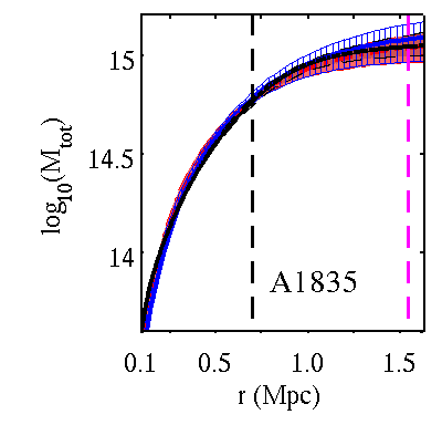
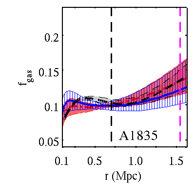
For these studies of cluster astrophysics, we continue to assume a fixed $d_{A}$ for each cluster. A test of how well this performs is presented in Figure 1.

3 Sensitivity to Angular Diameter Distance ($d_{A}$)

Rather than constraining $M_{\mbox{\scriptsize tot}}$ more precisely, we can relax the assumption of cosmology by including spectroscopic information in the joint fit. We consider here the cosmological sensitivity of our fits to the data.

The Compton $y$ parameter (Eq. 3), which scales as electron pressure integrated along sight line $\ell$, has an inverse linear dependence on $d_{A}$, since $d\ell=d_{A}\,d\theta$:

$$y=\frac{\mbox{$\sigma_{\mbox{\tiny T}}$}}{m_{e}c^{2}}\int\!\!P_{e}\,d\ell~{}~{}~{}\Rightarrow~{}~{}~{}P_{e}\propto d_{A}^{-1}.$$ (3)

Because X-ray imaging is sensitive to the surface brightness $S_{X}$ (Eq. 8), X-ray-constrained density is dependent on $d_{A}^{-1/2}$:

$$S_{X}=\frac{1}{4\pi(1+z)^{4}}\!\int\!\!n_{e}^{2}\mbox{$\Lambda_{ee}$}(T_{e},Z)\,d\ell~{}~{}~{}\Rightarrow~{}~{}~{}n_{e}\propto{d_{A}}^{-1/2}.$$ (4)

Combining these dependencies, we see

$$T_{\rm sl}\propto P_{e}/n_{e}\propto d_{A}^{-1/2}.$$ (5)

The spectroscopically-measured temperature $T_{X}$ does not have any dependence on $d_{A}$, so setting $T_{X}=T_{\rm sl}$ results in a ${d_{A}}^{-1/2}$ sensitivity to cosmology. This is the same cosmological sensitivity exploited in previous, joint X-ray+SZE $d_{A}$ determinations such as Bonamente et al. (2004), but relies on a more sophicated pair of models for the cluster gas.

Cluster $z$ $d_{A}$ $T_{X}$ $d_{A}$ $T_{\rm sl}$ (Mpc) (keV) (Mpc) (keV) A1835 0.25  806.5 $9.95^{+0.36}_{-0.37}$ $~{}867^{+140}_{-152}$ $9.99^{+0.57}_{-0.54}$ CL1226 0.89 1601.8 $9.30^{+1.33}_{-1.25}$ $1407^{+444}_{-321}$ $9.44^{+1.36}_{-1.08}$

Table 1: Clusters chosen for testing the ability of the upgraded N07+SVM profile to constrain cosmology.

The inverse square root cosmological sensitivity of a joint SZE+X-ray fit to a cluster implies that, for example, a single cluster observation with $\pm 10\%$ uncertainty in the measurements of $T_{\rm sl}$ and $T_{X}$ (the measurements of which should be independent) can constrain $d_{A}$ to within $\pm 37.6\%$. Here, I have added the errors on $T_{X}$ and $T_{\rm sl}$ in quadrature, since constraints provided by X-ray spectroscopic and the temperature derived from X-ray+SZE imaging should be independent. A determination of the angular diameter distance benefits from a large sample of clusters (e.g. Molnar et al. 2002; Bonamente et al. 2006), and we can expect a sample of $\sim 40$ relaxed clusters to yield $\sim 5\%$ statistical uncertainty on $d_{A}$ (where I have ignored systematics due to cluster asphericity and systematic effects in X-ray temperature measurements; see for example Ameglio et al. (2006)).

I tested this method on the relaxed clusters A1835 and CL1226, using the global $T_{X}$, measured within $r\in[0.15,1.0]\,r_{500}$, from Chapter 5. The results of this test are consistent with $\Lambda$CDMand are shown in Table 1.

It has been suggested (Alexey Vikhlinin, private communication) that a comparison between the X-ray proxy $Y_{X}\equiv\mbox{$M_{\mbox{\scriptsize gas}}$}T_{X}$ and the SZE quantity $Y_{\mbox{\scriptsize vol}}$ could be used to constrain $d_{A}$ more robustly than previous X-ray+SZE attempts, since both $Y_{X}$ and $Y_{\mbox{\scriptsize vol}}$ are integrated quantities that can be robustly determined. However, since the N07+SVM profiles share a density profile, simple inspection of Eq. 1 reveals that setting $T_{X}=T_{\rm sl}$ is in fact the correct implementation of comparison between $Y_{X}$ and $Y_{\mbox{\scriptsize vol}}$. The X-ray spectroscopic $T_{X}$ and the derived $T_{\rm sl}$ contain the same weighting by density, while $Y_{X}$ and $Y_{\mbox{\scriptsize vol}}$are not in general equivalent. Since $Y_{\mbox{\scriptsize vol}}$ is the integral of pressure, it scales as $\mbox{$M_{\mbox{\scriptsize gas}}$}T_{\rm mw}$, where $T_{\rm mw}$ is the mass-weighted temperature. In general, the emission-weighted temperature $T_{X}$ is not equivalent to the mass-weighted temperature, as $T_{X}$ favors denser regions more heavily than $T_{\rm mw}$ does, and clusters are not isothermal.

Recently, Allen et al. (2007) used X-ray observations of clusters to constrain $d_{A}$ by assuming the gas fraction $\mbox{$f_{\mbox{\scriptsize gas}}$}(r_{2500})$ is constant with redshift. They find $\mbox{$f_{\mbox{\scriptsize gas}}$}=\mbox{$M_{\mbox{\scriptsize gas}}$}/\mbox{$M_{\mbox{\scriptsize tot}}$}\propto d_{A}^{3/2}$, which is far more sensitive to $d_{A}$ than the line-of-sight SZE+X-ray joint fit when no assumptions are made about the evolution of $f_{\mbox{\scriptsize gas}}$.

For SZE+X-ray joint fits without spectroscopy, $M_{\mbox{\scriptsize gas}}$ has same dependence as it does when constrained by X-ray data alone, which is

$$M_{\rm gas}\propto n_{e}V\propto d_{A}^{5/2}.$$ (6)

Volume is proportional to the cube of angular diameter distance ($V\propto d_{A}^{3}$), and density is proportional to the inverse square-root of $d_{A}$ ($n_{e}\propto{d_{A}}^{-1/2}$, as implied by Eq. 4). For the $M_{\mbox{\scriptsize tot}}$ cosmological dependence, we have a slightly different cosmological dependence than that from X-ray alone:

$$M_{\rm tot}(r)=-\frac{r^{2}}{G\rho_{\rm gas}(r)}\left(\frac{dP_{\rm gas}}{dr}\right)\propto\frac{d_{A}^{2}}{d_{A}^{-1/2}}d_{A}^{-1}=d_{A}^{3/2},$$ (7)

using $r=\theta\,d_{A}$ and Eqs. 3 & 4. Since the SZE-determined pressure exhibits a different dependence on cosmology than the X-ray-determined pressure, we arrive at

$$f_{\rm gas}\propto d_{A}.$$ (8)

We conclude that an SZE+X-ray determination of $d_{A}$ using an assumed evolution of $f_{\mbox{\scriptsize gas}}$ would provide precisely the same sensitivity as Allen et al. (2007) exploit, since we recover an additional $d_{A}^{1/2}$ dependence through Eq. 5. However, the additional, independent constraints afforded by the inclusion of SZE data could provide a more precise determination than possible with X-ray data alone.

4 Final Words

In this thesis, I have presented an exciting new tool for observing the Sunyaev-Zel’dovich effect from galaxy clusters. I have shown how data from this – or any interferometric SZE instrument – can be combined with X-ray imaging to place reasonable constraints on galaxy clusters, including at high redshift where the SZE can contribute most significantly to the understanding of large scale structure. Finally, I have shown how the new models can be combined with X-ray spectroscopy to improve constraints and perform key measurements of the expansion of the Universe.

Part 3 Appendix

Chapter 7 Chandra X-ray Data Analysis

The X-ray data used in this analysis were obtained with the Chandra ACIS-I detector, which provides spatially resolved X-ray spectroscopy and imaging with an angular resolution of $0.492\arcsec$ and with energy resolution of $\sim$ 100-200 eV. Data analysis was performed with the CIAO software (version 3.2) and the CALDB calibration information (version 3.1) provided by the Chandra calibration team.

Both images and spectra of the low-redshift clusters were limited to the 0.7–7.0 keV energy band in order to exclude the low-energy and high-energy data that are more strongly affected by background and by calibration uncertainties. For the high-redshift cluster, CL1226 ($z=0.89$), the image was limited to the 0.7–2.0 keV band, where Chandra’s efficiency peaks (see Fig. 12). This range of energies was chosen because, with a spectroscopic temperature of $\sim$9.8 keV, only $\sim 50\%$ of the redshifted cluster emission is measured at photon energies $\gtrsim 2$ keV; However, the X-ray background in a 0.7–7.0 keV image is $\sim 4$ times higher than that in a 0.7–2.0 keV image. Combining this with the fact that the ACIS-I efficiency peaks below 2 keV (see Fig. 12), the highest $S/N$ is obtained in the detector energy range 0.7–2.0 keV.

The X-ray images were binned in 1.968$\arcsec$ pixels; this sets the limiting angular resolution of our X-ray data, as the Chandra point spread function in the center of the X-ray image is smaller than our adopted pixel size. The X-ray background was measured for each cluster exposure, using peripheral regions of the adjacent detector ACIS-I chips that are source free. Additional details of the Chandra X-ray data analysis are presented in Bonamente et al. (2004, 2006).

References

- Afshordi et al. (2007) Afshordi, N., Lin, Y.-T., Nagai, D., & Sanderson, A. J. R. 2007, MNRAS, 378, 293
- Albrecht et al. (2006) Albrecht, A., Bernstein, G., Cahn, R., Freedman, W. L., Hewitt, J., Hu, W., Huth, J., Kamionkowski, M., Kolb, E. W., Knox, L., Mather, J. C., Staggs, S., & Suntzeff, N. B. 2006, ArXiv Astrophysics e-prints
- Allen et al. (2007) Allen, S. W., Rapetti, D. A., Schmidt, R. W., Ebeling, H., Morris, G., & Fabian, A. C. 2007, ArXiv e-prints, 706
- Allen et al. (2004) Allen, S. W., Schmidt, R. W., Ebeling, H., Fabian, A. C., & van Speybroeck, L. 2004, MNRAS, 353, 457
- Ameglio et al. (2006) Ameglio, S., Borgani, S., Diaferio, A., & Dolag, K. 2006, MNRAS, 369, 1459
- Anders & Grevesse (1989) Anders, E. & Grevesse, N. 1989, Geochim. Cosmochim. Acta, 53, 197
- Arnaud (1996) Arnaud, K. A. 1996, in Astronomical Data Analysis Software and Systems V, ed. G. H. Jacoby & J. Barnes, 17
- Best et al. (1995) Best, N. G., Cowles, M. K., & Vines, S. K. 1995, CODA Manual Version 0.30 (MRC Biostatic Unit, Cambridge, UK)
- Bonamente et al. (2008) Bonamente, M., Joy, M., LaRoque, S. J., Carlstrom, J. E., Nagai, D., & Marrone, D. P. 2008, ApJ, 675, 106
- Bonamente et al. (2004) Bonamente, M., Joy, M. K., Carlstrom, J. E., Reese, E. D., & LaRoque, S. J. 2004, ApJ, 614, 56
- Bonamente et al. (2006) Bonamente, M., Joy, M. K., LaRoque, S. J., Carlstrom, J. E., Reese, E. D., & Dawson, K. S. 2006, ApJ, 647, 25
- Bracewell (2000) Bracewell, R. N. 2000, The Fourier Transform and its Applications (The Fourier Transform and its Applications / Ronald N. Bracewell. Boston : McGraw Hill, c2000. (McGraw-Hill series in electrical and computer engineering. Circuits and systems))
- Carlstrom et al. (1998) Carlstrom, J. E., Grego, L., Holzapfel, W. L., & Joy, M. 1998, Eighteenth Texas Symposium on Relativistic Astrophysics and Cosmology, ed A. Olinto, J. Frieman, and D. Schramm, World Scientific, 261
- Carlstrom et al. (2002) Carlstrom, J. E., Holder, G. P., & Reese, E. D. 2002, ARA&A, 40, 643
- Carlstrom et al. (2000) Carlstrom, J. E., Joy, M. K., Grego, L., Holder, G. P., Holzapfel, W. L., Mohr, J. J., Patel, S., & Reese, E. D. 2000, Physica Scripta Volume T, 85, 148
- Cavaliere & Fusco-Femiano (1976) Cavaliere, A. & Fusco-Femiano, R. 1976, A&A, 49, 137
- Cavaliere & Fusco-Femiano (1978) —. 1978, A&A, 70, 677
- Condon et al. (1998) Condon, J. J., Cotton, W. D., Greisen, E. W., Yin, Q. F., Perley, R. A., Taylor, G. B., & Broderick, J. J. 1998, AJ, 115, 1693
- da Silva et al. (2004) da Silva, A. C., Kay, S. T., Liddle, A. R., & Thomas, P. A. 2004, MNRAS, 348, 1401
- David et al. (1995) David, L. P., Jones, C., & Forman, W. 1995, ApJ, 445, 578
- Ebeling et al. (2001) Ebeling, H., Edge, A. C., & Henry, J. P. 2001, ApJ, 553, 668
- Ettori (2001) Ettori, S. 2001, in Astronomical Society of the Pacific Conference Series, Vol. 245, Astrophysical Ages and Times Scales, ed. T. von Hippel, C. Simpson, & N. Manset, 500–+
- Gilks et al. (1996) Gilks, W. R., Richardson, S., & Spiegelhalter, D. J. 1996, Markov Chain Monte Carlo in Practice (Chapman and Hall)
- Grego (1999) Grego, L. 1999, PhD thesis, California Institute of Technology
- Grego et al. (2000) Grego, L., Carlstrom, J. E., Joy, M. K., Reese, E. D., Holder, G. P., Patel, S., Cooray, A. R., & Holzapfel, W. L. 2000, ApJ, 539, 39
- Grego et al. (2001) Grego, L., Carlstrom, J. E., Reese, E. D., Holder, G. P., Holzapfel, W. L., Joy, M. K., Mohr, J. J., & Patel, S. 2001, ApJ, 552, 2
- Haiman et al. (2001) Haiman, Z., Mohr, J. J., & Holder, G. P. 2001, ApJ, 553, 545
- Hawkins et al. (2004) Hawkins, D. W., Woody, D. P., Wiitala, B., Fredsti, J., & Rauch, K. P. 2004, in Presented at the Society of Photo-Optical Instrumentation Engineers (SPIE) Conference, Vol. 5498, Millimeter and Submillimeter Detectors for Astronomy II. Edited by Jonas Zmuidzinas, Wayne S. Holland and Stafford Withington Proceedings of the SPIE, Volume 5498, pp. 567-578 (2004)., ed. C. M. Bradford, P. A. R. Ade, J. E. Aguirre, J. J. Bock, M. Dragovan, L. Duband, L. Earle, J. Glenn, H. Matsuhara, B. J. Naylor, H. T. Nguyen, M. Yun, & J. Zmuidzinas, 567–578
- Hinshaw et al. (2008) Hinshaw, G., Weiland, J. L., Hill, R. S., Odegard, N., Larson, D., Bennett, C. L., Dunkley, J., Gold, B., Greason, M. R., Jarosik, N., Komatsu, E., Nolta, M. R., Page, L., Spergel, D. N., Wollack, E., Halpern, M., Kogut, A., Limon, M., Meyer, S. S., Tucker, G. S., & Wright, E. L. 2008, ArXiv e-prints, 803
- Holder et al. (2000) Holder, G. P., Mohr, J. J., Carlstrom, J. E., Evrard, A. E., & Leitch, E. M. 2000, ApJ, 544, 629
- Itoh et al. (1998) Itoh, N., Kohyama, Y., & Nozawa, S. 1998, ApJ, 502, 7
- Jing & Suto (2000) Jing, Y. P. & Suto, Y. 2000, ApJ, 529, L69
- Joy et al. (2001) Joy, M., LaRoque, S., Grego, L., Carlstrom, J. E., Dawson, K., Ebeling, H., Holzapfel, W. L., Nagai, D., & Reese, E. D. 2001, ApJ, 551, L1
- Kaastra & Mewe (1993) Kaastra, J. S. & Mewe, R. 1993, A&AS, 97, 443
- Kravtsov et al. (2005) Kravtsov, A. V., Nagai, D., & Vikhlinin, A. A. 2005, ApJ, 625, 588
- Kravtsov et al. (2006) Kravtsov, A. V., Vikhlinin, A., & Nagai, D. 2006, ApJ, 650, 128
- LaRoque et al. (2006) LaRoque, S. J., Bonamente, M., Carlstrom, J. E., Joy, M. K., Nagai, D., Reese, E. D., & Dawson, K. S. 2006, ApJ, 652, 917
- LaRoque et al. (2003) LaRoque, S. J., Joy, M., Carlstrom, J. E., Ebeling, H., Bonamente, M., Dawson, K. S., Edge, A., Holzapfel, W. L., Miller, A. D., Nagai, D., Patel, S. K., & Reese, E. D. 2003, ApJ, 583, 559
- Leitch et al. (2005) Leitch, E. M., Carlstrom, J. E., Davidson, G., Dragovan, M., Halverson, N. W., Holzapfel, W. L., Laroque, S., Kovac, J., Pryke, C., Schartman, E., & Yamasaki, M. J. 2005, in IAU Symposium, Vol. 201, New Cosmological Data and the Values of the Fundamental Parameters, ed. A. N. Lasenby & A. Wilkinson, 33–+
- Liedahl et al. (1995) Liedahl, D. A., Osterheld, A. L., & Goldstein, W. H. 1995, ApJ, 438, L115
- Loken et al. (2002) Loken, C., Norman, M. L., Nelson, E., Burns, J., Bryan, G. L., & Motl, P. 2002, ApJ, 579, 571
- Longair (1998) Longair, M. S., ed. 1998, Galaxy formation
- Markevitch et al. (1998) Markevitch, M., Forman, W. R., Sarazin, C. L., & Vikhlinin, A. 1998, ApJ, 503, 77
- Maughan (2007) Maughan, B. J. 2007, ArXiv Astrophysics e-prints
- Maughan et al. (2008) Maughan, B. J., Jones, C., Forman, W., & Van Speybroeck, L. 2008, ApJS, 174, 117
- Maughan et al. (2007) Maughan, B. J., Jones, C., Jones, L. R., & Van Speybroeck, L. 2007, ApJ, 659, 1125
- Mazzotta et al. (2004) Mazzotta, P., Rasia, E., Moscardini, L., & Tormen, G. 2004, MNRAS, 354, 10
- Mewe et al. (1985) Mewe, R., Gronenschild, E. H. B. M., & van den Oord, G. H. J. 1985, A&AS, 62, 197
- Molnar et al. (2002) Molnar, S. M., Birkinshaw, M., & Mushotzky, R. F. 2002, ApJ, 570, 1
- Moore et al. (1999) Moore, B., Quinn, T., Governato, F., Stadel, J., & Lake, G. 1999, MNRAS, 310, 1147
- Mroczkowski et al. (2008) Mroczkowski, T., Bonamente, M., Carlstrom, J. E., Culverhouse, T. L., Greer, C., Hawkins, D., Hennessy, R., Joy, M., Lamb, J. W., Leitch, E. M., Loh, M., Maughan, B., Marrone, D. P., Miller, A., Nagai, D., Muchovej, S., Pryke, C., Sharp, M., & Woody, D. 2008, ArXiv e-prints
- Muchovej (2008) Muchovej, S. 2008, PhD thesis, Columbia University
- Muchovej et al. (2007) Muchovej, S., Mroczkowski, T., Carlstrom, J. E., Cartwright, J., Greer, C., Hennessy, R., Loh, M., Pryke, C., Reddall, B., Runyan, M., Sharp, M., Hawkins, D., Lamb, J. W., Woody, D., Joy, M., Leitch, E. M., & Miller, A. D. 2007, ApJ, 663, 708
- Mushotzky & Scharf (1997) Mushotzky, R. F. & Scharf, C. A. 1997, ApJ, 482, L13+
- Nagai (2006) Nagai, D. 2006, ApJ, 650, 538
- Nagai et al. (2007a) Nagai, D., Kravtsov, A. V., & Vikhlinin, A. 2007a, ApJ, 668, 1
- Nagai et al. (2007b) Nagai, D., Vikhlinin, A., & Kravtsov, A. V. 2007b, ApJ, 655, 98
- Navarro et al. (1997) Navarro, J. F., Frenk, C. S., & White, S. D. M. 1997, ApJ, 490, 493
- Neumann (2006) Neumann, D. M. 2006, in EAS Publications Series, Vol. 20, EAS Publications Series, ed. G. A. Mamon, F. Combes, C. Deffayet, & B. Fort, 179–182
- NIST (2008) NIST. 2008, Cryogenic Technologies Group – Cryogenics Material Properties, http://www.cryogenics.nist.gov/MPropsMAY/material%20properties.htm
- Oppenheim et al. (1999) Oppenheim, A. V., Schafer, R. W., & Buck, J. R. 1999, Discrete-time signal processing (2nd ed.) (Upper Saddle River, NJ, USA: Prentice-Hall, Inc.)
- Patel et al. (2000) Patel, S. K., Joy, M., Carlstrom, J. E., Holder, G. P., Reese, E. D., Gomez, P. L., Hughes, J. P., Grego, L., & Holzapfel, W. L. 2000, ApJ, 541, 37
- Peterson et al. (2001) Peterson, J. R., Paerels, F. B. S., Kaastra, J. S., Arnaud, M., Reiprich, T. H., Fabian, A. C., Mushotzky, R. F., Jernigan, J. G., & Sakelliou, I. 2001, A&A, 365, L104
- Pfrommer et al. (2007) Pfrommer, C., Enßlin, T. A., Springel, V., Jubelgas, M., & Dolag, K. 2007, MNRAS, 378, 385
- Piffaretti et al. (2005) Piffaretti, R., Jetzer, P., Kaastra, J. S., & Tamura, T. 2005, A&A, 433, 101
- Plummer et al. (2006) Plummer, M., Best, N. G., Cowles, M. K., & Vines, S. K. 2006, R News, 6, 7
- Pratt & Arnaud (2002) Pratt, G. W. & Arnaud, M. 2002, A&A, 394, 375
- Pratt et al. (2007) Pratt, G. W., Böhringer, H., Croston, J. H., Arnaud, M., Borgani, S., Finoguenov, A., & Temple, R. F. 2007, A&A, 461, 71
- Raftery & Lewis (1992) Raftery, A. L. & Lewis, S. 1992, in Bayesian Statistics IV, ed. J. M. Bernardo & M. H. DeGroot (Oxford University Press), 763
- Rapetti & Allen (2007) Rapetti, D. & Allen, S. W. 2007, ArXiv e-prints, 710
- Raymond & Smith (1977) Raymond, J. C. & Smith, B. W. 1977, ApJS, 35, 419
- Reese et al. (2002) Reese, E. D., Carlstrom, J. E., Joy, M., Mohr, J. J., Grego, L., & Holzapfel, W. L. 2002, ApJ, 581, 53
- Reese et al. (2000) Reese, E. D., Mohr, J. J., Carlstrom, J. E., Joy, M., Grego, L., Holder, G. P., Holzapfel, W. L., Hughes, J. P., Patel, S. K., & Donahue, M. 2000, ApJ, 533, 38
- Riess et al. (1998) Riess, A. G., Filippenko, A. V., Challis, P., Clocchiatti, A., Diercks, A., Garnavich, P. M., Gilliland, R. L., Hogan, C. J., Jha, S., Kirshner, R. P., Leibundgut, B., Phillips, M. M., Reiss, D., Schmidt, B. P., Schommer, R. A., Smith, R. C., Spyromilio, J., Stubbs, C., Suntzeff, N. B., & Tonry, J. 1998, AJ, 116, 1009
- Rohlfs & Wilson (1996) Rohlfs, K. & Wilson, T. L. 1996, Tools of Radio Astronomy, 2nd edn. (Berlin: Springer)
- Sarazin (1988) Sarazin, C. L. 1988, X-ray Emission From Clusters of Galaxies (Cambridge University Press)
- Scott & Pound (2006) Scott, S. L. & Pound, M. W. 2006, in Astronomical Society of the Pacific Conference Series, Vol. 351, Astronomical Data Analysis Software and Systems XV, ed. C. Gabriel, C. Arviset, D. Ponz, & S. Enrique, 670–+
- Shepherd (1997) Shepherd, M. C. 1997, in Astronomical Society of the Pacific Conference Series, Vol. 125, Astronomical Data Analysis Software and Systems VI, ed. G. Hunt & H. Payne, 77–+
- Smith et al. (2001) Smith, R. K., Brickhouse, N. S., Liedahl, D. A., & Raymond, J. C. 2001, ApJ, 556, L91
- Spergel et al. (2003) Spergel, D. N., Verde, L., Peiris, H. V., Komatsu, E., Nolta, M. R., Bennett, C. L., Halpern, M., Hinshaw, G., Jarosik, N., Kogut, A., Limon, M., Meyer, S. S., Page, L., Tucker, G. S., Weiland, J. L., Wollack, E., & Wright, E. L. 2003, ApJS, 148, 175
- Struble & Rood (1999) Struble, M. F. & Rood, H. J. 1999, ApJS, 125, 35
- Thompson et al. (2001) Thompson, A. R., Moran, J. M., & Swenson, G. W. 2001, Interferometry and Synthesis in Radio Astronomy (Wiley-Interscience, 2nd ed.)
- van Speybroeck (1999) van Speybroeck, L. 1999, American Astronomical Society Meeting, 31, 917
- Vikhlinin (2006) Vikhlinin, A. 2006, ApJ, 640, 710
- Vikhlinin et al. (2008) Vikhlinin, A., Burenin, R. A., Ebeling, H., Forman, W. R., Hornstrup, A., Jones, C., Kravtsov, A. V., Murray, S. S., Nagai, D., Quintana, H., & Voevodkin, A. 2008, ArXiv e-prints, 805
- Vikhlinin et al. (2006) Vikhlinin, A., Kravtsov, A., Forman, W., Jones, C., Markevitch, M., Murray, S. S., & Van Speybroeck, L. 2006, ApJ, 640, 691
- Vikhlinin et al. (2005) Vikhlinin, A., Markevitch, M., Murray, S. S., Jones, C., Forman, W., & Van Speybroeck, L. 2005, ApJ, 628, 655
- White et al. (1997) White, R. L., Becker, R. H., Helfand, D. J., & Gregg, M. D. 1997, ApJ, 475, 479
- White et al. (1993) White, S. D. M., Navarro, J. F., Evrard, A. E., & Frenk, C. S. 1993, Nature, 366, 429
- Woodcraft (2005) Woodcraft, A. L. 2005, Cryogenics, 45, 626
- Woody et al. (2004) Woody, D. P., Beasley, A. J., Bolatto, A. D., Carlstrom, J. E., Harris, A., Hawkins, D. W., Lamb, J., Looney, L., Mundy, L. G., Plambeck, R. L., Scott, S., & Wright, M. 2004, in Presented at the Society of Photo-Optical Instrumentation Engineers (SPIE) Conference, Vol. 5498, Millimeter and Submillimeter Detectors for Astronomy II. Edited by Jonas Zmuidzinas, Wayne S. Holland and Stafford Withington Proceedings of the SPIE, Volume 5498, pp. 30-41 (2004)., ed. C. M. Bradford, P. A. R. Ade, J. E. Aguirre, J. J. Bock, M. Dragovan, L. Duband, L. Earle, J. Glenn, H. Matsuhara, B. J. Naylor, H. T. Nguyen, M. Yun, & J. Zmuidzinas, 30–41