A Computational and Theoretical Investigation of the Accuracy of Quasicontinuum Methods

Abstract.

We give computational results to study the accuracy of several quasicontinuum methods for two benchmark problems — the stability of a Lomer dislocation pair under shear and the stability of a lattice to plastic slip under tensile loading. We find that our theoretical analysis of the accuracy near instabilities for one-dimensional model problems can successfully explain most of the computational results for these multi-dimensional benchmark problems. However, we also observe some clear discrepancies, which suggest the need for additional theoretical analysis and benchmark problems to more thoroughly understand the accuracy of quasicontinuum methods.

1. Introduction

Multiphysics model coupling has captured the excitement of the engineering research community for its potential to make possible the numerical simulation of heretofore computationally inaccessible multiscale problems. The capability to assess the accuracy of these multiphysics methods is crucial to both the verification of existing methods and the development of improved methods.

During the past several years, a theoretical basis has been developed for estimating the error of atomistic-to-continuum coupling methods  [27, 21, 22, 23, 2, 34, 36, 10, 11, 32, 25, 26, 35, 16, 19, 24, 3, 29, 13, 12, 9, 8]. However, the accurate computation of lattice instabilities such as dislocation formation and movement, crack propagation, and plastic slip are primary goals of atomistic-to-continuum coupling methods; and a theoretical analysis of the accuracy of atomistic-to-coupling methods up to the onset of lattice instability of the atomistic energy has thus far only been achieved for one-dimensional model problems [14, 12, 34, 11, 5, 35]. This theoretical analysis and corresponding numerical experiments have given a precise understanding of the varying accuracy of these methods for simple model problems, but it is not known to what degree these errors are significant for the multi-dimensional problems of scientific and technological interest.

We have developed a benchmark test code to study the atomistic-to-continuum coupling error for a face-centered cubic (FCC) crystal. Following the benchmark investigation of Miller and Tadmor [31], the displacement $U\left(x_{1},\,x_{2},\,x_{3}\right)$ of the atoms from their reference lattice positions is constrained by the atomistic analogue of continuum “plane strain” symmetry:

$$U=\left(U_{1},\,U_{2},\,0\right)\quad\text{and}\quad U\left(x_{1},\,x_{2},\,x_{3}\right)=u\left(x_{1},\,x_{2}\right)$$

where the crystal coordinates are given in terms of the basis vectors defined using Miller indices[1] by $e_{1}=$[1 1 0], $e_{2}=$[0 0 1], and $e_{3}=$[1 -1 0]. We note that the computation of the atomistic energy and forces for an atomistic displacement with plane strain symmetry requires the summation of the interaction of each atom with neighboring atoms in three-dimensional space.

We have recomputed the benchmark study of Miller and Tadmor [31] for the Lomer dislocation dipole to more clearly separate the errors due to continuum modeling error, atomistic-to-continuum coupling error, and solution error. We allow a more general atomistic domain that is fully surrounded by a continuum region. We have also investigated plastic slip for tensile loading. Further investigation is underway to study the coarsening error in the continuum region and the far-field boundary condition error.

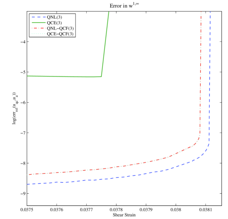
We have found that the patch-test consistent quasi-nonlocal (QNL) method  [40] gave a more accurate critical shear strain than the popular “ghost force correction” quasicontinuum coupling method  [30, 38] tested in [31] (see Table 1 and Figure 7). This result confirms our earlier theoretical analysis of the dependence of the critical shear strain error on the accuracy of the atomistic-to-continuum coupling [14].

The motivation for the ghost force correction method (equation (2.12) below) was to correct the large coupling errors of the original quasicontinuum method (QCE)  [41] by applying a “dead load” correction  [30, 38, 31]. We have recast the ghost force correction method in a numerical analysis setting as an iterative method to solve the equilibrium equations for the force-based quasicontinuum (QCF) method  [8, 9], and we have proven for a one-dimensional model problem that the ghost force correction (QCE-QCF) method is inaccurate near lattice instabilities because it uses the patch-test inconsistent QCE method as a preconditioner for the QCF equilibrium equations [15]. The benchmark tests we present here confirm that the QCE-QCF method is not as accurate as the QNL method near lattice instabilities.

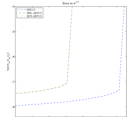
By contrast, we found that the $w^{1,\infty}$ error was smaller for the QNL method than for the QCE-QCF method far from lattice instabilities (see Figures 7-9), which is contrary to expectations based on our analyses of a 1D model in [13, 15, 34, 11], where we have shown that the QCF method (the limit of the QCE-QCF iteration) is a more accurate approximation than the QNL method.

Another result of our numerical experiments that contradicts our 1D analysis [15] is that near a slip instability the QCE-QCF method has comparable accuracy to the QNL-QCF method, which uses the QNL energy as a preconditioner. To explain this, we note that our 1D analysis in [15] can be considered a good model for cleavage fracture, but not for the slip instabilities studied in the present paper. We are currently attempting to develop a 2D benchmark test for cleavage fracture to demonstrate that the QCE-QCF method may be less accurate than the QNL-QCF method near some types of lattice instabilities.

2. The atomistic and quasicontinuum models

2.1. A model for plane strain in the face centered cubic lattice

Let ${\mathcal{L}}$ be a face centered cubic (fcc) lattice [1] with cube side length $a$ and nearest-neighbor distance $a/\sqrt{2}$ . Our plane strain model is most easily derived by viewing the fcc lattice ${\mathcal{L}}$ as being generated by the primitive lattice vectors

$$a_{1}=\frac{a}{2}(0,\,1,\,1),\quad a_{2}=\frac{a}{2}(1,\,0,\,1),\quad\text{and}\quad a_{3}=\frac{a}{2}(1,\,1,\,0).$$ (2.1)

The cubic supercells are then generated by the cubic lattice vectors

$$\begin{gathered}A_{1}=a(1,\,0,\,0)=-a_{1}+a_{2}+a_{3},\quad A_{2}=a(0,\,1,\,0)=a_{1}-a_{2}+a_{3},\\ A_{3}=a(0,\,0,\,1)=a_{1}+a_{2}-a_{3}.\end{gathered}$$ (2.2)

We let ${P}$ be the orthogonal projection of ${\mathcal{L}}$ onto the plane with normal given by $a_{1}-a_{2}=\frac{a}{2}(-1,\,1,\,0)$ (or the ${\hkl(1-10)}$ plane using Miller indices since we have that $A_{1}-A_{2}=-2(a_{1}-a_{2})$), and let ${Q}=I-{P}$ be the projection onto the line parallel to $a_{1}-a_{2}=\frac{a}{2}(-1,\,1,\,0)$ (or the ${\hkl[1-10]}$ direction using Miller indices [1]). We observe that the projection of ${\mathcal{L}}$ onto the plane normal to $a_{1}-a_{2}=\frac{a}{2}(-1,\,1,\,0)$ (or the ${\hkl(1-10)}$ plane using Miller indices) is a triangular lattice ${\mathcal{T}}:={P}{\mathcal{L}}$. Each point in the triangular lattice ${\mathcal{T}}:={P}{\mathcal{L}}$ is thus the projection of a column of atoms with spacing $a/\sqrt{2}$ parallel to $a_{1}-a_{2}=\frac{a}{2}(-1,\,1,\,0)$ (or the ${\hkl[1-10]}$ direction using Miller indices) as depicted in Figure 1.

Figure 1. Illustration of the FCC lattice and the projection onto the ${\hkl(1-10)}$ plane. The grey shaded region represents the ${\hkl(1-10)}$ plane, the asterisks are the points in the triangular lattice ${\mathcal{T}}$, and the disks are the atoms in the FCC lattice $\mathcal{L}$. The vertical lines emanating from the points in ${\mathcal{T}}$ represent the columns of atoms in the FCC lattice which project onto points of ${\mathcal{T}}$. The reader should imagine that there is a vertical column of atoms emanating from each point of ${\mathcal{T}}$.

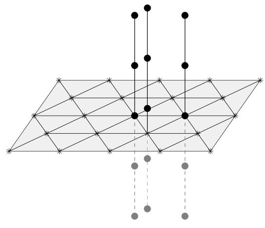
Now let ${\omega}$ be a finite subset of the triangular lattice ${\mathcal{T}}$, and let ${\Omega}$ be the right cylinder over ${\omega}$ in the fcc lattice ${\mathcal{L}}$. We will call a displacement $U:{\Omega}\rightarrow\mathbb{R}^{3}$ periodic if

$$U(X)=U\bigg{(}X+n(a_{1}-a_{2})\bigg{)}\quad\text{ for all }X\in{\Omega}\text{ and all }n\in{\mathbb{Z}}.$$

We note that the scale of the periodicity is $|a_{1}-a_{2}|=a/\sqrt{2}.$ Any periodic displacement $U$ reduces to a displacement ${u}:{\omega}\rightarrow\mathbb{R}^{3}$ defined by

$${u}(x):=U(X)\quad\text{ for any }X\in{\Omega}\text{ with }{P}X=x.$$

We let ${\mathcal{U}}$ denote the space of displacements of ${\omega}$.

We will now derive an energy per period $\mathcal{E}^{a}:{\mathcal{U}}\rightarrow\mathbb{R}$ and a corresponding force field on ${\omega}.$ Let ${\phi}$ be a pair potential. For example, we use the Morse potential in our numerical experiments below. We will adopt a fourth-nearest neighbor pair-interaction model. For this choice of the interaction model the quasi-nonlocal coupling method [40] can be applied. We note that, throughout, we understand $n$-th nearest neighbours in terms of Euclidean distance in the reference configuration in $\mathbb{R}^{3}$ (i.e., in the 3D FCC lattice) [40].

Let ${\mathcal{M}}$ denote the ${\mathcal{L}}$-interaction range, by which we mean the set of all vectors pointing from an atom in ${\mathcal{L}}$ to one of its first, second, third, or fourth nearest-neighbors. Representative first, second, third, or fourth nearest-neighbor vectors are given in terms of the primitive lattice vectors (2.1) and cubic lattice vectors (2.2) by

$$a_{1}=\left(0,\,\frac{a}{2},\,\frac{a}{2}\right),\quad A_{1}=\left(a,\,0,\,0\right),\quad a_{2}+a_{3}=\left(a,\,\frac{a}{2},\,\frac{a}{2}\right),\quad 2a_{1}=\left(0,\,a,\,a\right),$$ (2.3)

with the full set of first, second, third, or fourth nearest-neighbor vectors given by symmetry.

For $X\in{\Omega},$ we let

$${\mathcal{M}}_{X}:=\{B\in{\mathcal{M}}:X+B\in{\Omega}\}.$$

We will often call directions $B\in{\mathcal{M}}_{X}$ bonds. We note that ${\mathcal{M}}\neq{\mathcal{M}}_{X}$ when $X$ lies in a shallow layer along the boundary of ${\Omega}.$ We also note that we have ${\mathcal{M}}_{X_{1}}={\mathcal{M}}_{X_{2}}$ if $PX_{1}=PX_{2}=x,$ hence we can unambiguously use the notation ${\mathcal{M}}_{x}:={\mathcal{M}}_{X}$ where $PX=x$ for $x\in{\omega}.$

For any $B\in{\mathcal{M}}$ and any displacement $U(X),$ we define the difference operator $D_{B}$ by

$$D_{B}U(X):=U(X+B)-U(X),$$

whenever $X,\ X+B\in{\Omega}$. We define the set of projections $b=PB$ of the bonds in ${\mathcal{M}}$ and ${\mathcal{M}}_{X}$ onto the plane ${\hkl(1-10)}$ by

$${\mathcal{R}}:=P{\mathcal{M}}\qquad\text{and}\qquad{\mathcal{R}}_{x}:=P{\mathcal{M}}_{X}.$$

For periodic displacements $U(X),$ we define

$$D_{b}u(x):=u(x+b)-u(x)=U(X+B)-U(X)=D_{B}U(X)$$

where $u(x)=U(X)$ for $x=PX$ and $b=PB.$ It will also be convenient to use the notation

$$D_{B}u(x):=D_{b}u(x)=D_{B}U(X)\quad\text{for }PB=b.$$

The energy per period $\mathcal{E}^{a}:{\mathcal{U}}\rightarrow\mathbb{R}$ is given by

$$\mathcal{E}^{a}(u):={\textstyle\frac{1}{2}}\sum_{x\in{\omega}}\sum_{B\in{\mathcal{M}}_{x}}{\phi}(|B+D_{B}u(x)|)$$

where we note that the difference in the deformed positions of atoms at $X+B$ and $X$ is $B+D_{B}u(x).$ The corresponding force at $x\in{\omega}$ is then given by

$${\mathcal{F}}^{a}(u)(x):=-\frac{\partial}{\partial u(x)}\mathcal{E}^{a}(u)(x)=-\frac{\partial}{\partial u(x)}\sum_{B\in{\mathcal{M}}_{x}}{\phi}(|B+D_{B}u(x)|),$$ (2.4)

where $\frac{\partial}{\partial u(x)}$ above denotes the partial derivative with respect to the displacement $u(x)$ of the atom with projected reference position $x\in{\omega}.$ We define the first variation (or, gradient) of $\mathcal{E}^{a}(u)$ by $\delta\mathcal{E}^{a}(u),$ which is given for each $x\in{\omega}$ by

$$\delta\mathcal{E}^{a}(u)(x):=\frac{\partial}{\partial u(x)}\mathcal{E}^{a}(u)(x).$$ (2.5)

We can then express (2.4) in operator notation by

$${\mathcal{F}}^{a}(u)=-\delta\mathcal{E}^{a}(u).$$

We will now formulate a boundary value problem for the energy $\mathcal{E}^{a}$. We let $\Gamma\subset{\omega}$ denote the part of the “boundary” where the displacements are constrained. In the numerical experiments described below, $\Gamma$ will be a shallow layer of atoms along all or some of the boundary of ${\omega}$. Let the space of admissible displacements that are equal to ${u}_{0}\in{\mathcal{U}}$ on the boundary $\Gamma$ be denoted by

$${\rm Adm}({u}_{0}):=\{{u}\in{\mathcal{U}}:{u}(x)={u}_{0}(x)\text{ for all }x\in\Gamma\}.$$

We will study the minimization problem (or more precisely, the local minimization problem):

$$\text{Find }{u}\in\operatorname*{arg\ local\ min}_{v\in{\rm Adm}({u}_{0})}\mathcal{E}^{a}(v).$$ (2.6)

The Euler–Lagrange equation corresponding to problem (2.6) is

$$-\delta\mathcal{E}^{a}({u})(x) =0 \quad\text{ for all }x\in{\omega}\setminus\Gamma,$$

$${u}(x) ={u}_{0}(x) \quad\text{ for all }x\in\Gamma.$$

In our numerical experiments, we consider only initial displacements $u_{0}$ satisfying $u_{0}:{\omega}\rightarrow{\hkl(1-10)},$ where we recall that ${\hkl(1-10)}$ is the plane with normal given by $a_{1}-a_{2}=\frac{a}{2}(-1,\,1,\,0)$. We will call any displacement $u:{\omega}\rightarrow{\hkl(1-10)}$ a plane displacement, and we will let $\mathcal{V}\subset{\mathcal{U}}$ denote the space of plane displacements. For plane displacements, $\mathcal{E}^{a}$ can be interpreted as the energy of the two dimensional crystal ${\omega}$ computed using a pair potential which depends on the bond direction.

The restriction of the energy per period $\mathcal{E}^{a}(u):{\mathcal{U}}\rightarrow\mathbb{R}$ to plane displacements $\mathcal{V}$ can then be given by

$$\mathcal{E}^{a}(u)={\textstyle\frac{1}{2}}\sum_{x\in{\omega}}\sum_{b\in{\mathcal{R}}_{x}}{\phi}_{b}(|b+D_{b}u(x)|),\quad u\in\mathcal{V},$$ (2.7)

where ${\phi}_{b}:(0,\infty)\rightarrow\mathbb{R}$ is given by

$${\phi}_{b}(r):=\sum_{\{B\in{\mathcal{M}}_{x}:\,{P}B=b\}}{\phi}\left(\left(r^{2}+|{Q}B|^{2}\right)^{1/2}\right)$$

where we recall that ${Q}=I-P$ is the projection onto the line parallel to $a_{1}-a_{2}=\frac{a}{2}(-1,\,1,\,0).$ Roughly speaking, ${\phi}_{b}(|b+D_{b}u(x)|)$ is the energy of the interaction of atom $x$ with all of its neighbors in the column over $x+b.$ For $x\in{\omega}$, we will call the inner sum

$$\mathcal{E}^{a}_{x}(u):={\textstyle\frac{1}{2}}\sum_{b\in{\mathcal{R}}_{x}}{\phi}_{b}(|b+D_{b}u(x)|)$$

the atomistic energy at $x$.

It will be convenient to establish coordinates adapted to the triangular lattice ${\mathcal{T}}$, which lies in the plane defined by the normal $a_{1}-a_{2}=\frac{a}{2}(-1,\,1,\,0)$ (or the ${\hkl(1-10)}$ plane). This plane is spanned by the orthogonal vectors of length $a/\sqrt{2}$ in the $\hkl[110]$ direction and of length $a$ in the $\hkl[001]$ direction given by

$$\begin{split}V_{1}:&={\textstyle\frac{1}{2}}(A_{1}+A_{2})=a_{3}={\textstyle\frac{a}{2}}(1,\,1,\,0),\\ V_{2}:&=A_{3}=a_{1}+a_{2}-a_{3}=a(0,\,0,\,1).\end{split}$$

Throughout the remainder of this paper, we will denote the coordinates of $(x_{1},x_{2})$ in the $\{\,V_{1},\,V_{2}\,\}$ basis by

$$\langle\nu_{1},\nu_{2}\rangle:=\nu_{1}V_{1}+\nu_{2}V_{2}.$$

The triangular lattice ${\mathcal{T}}$ is then generated by the basis vectors $\langle 1,\,0\rangle$ and $\langle 1/2,\,1/2\rangle.$

It can be checked that there are four distinct symmetry-related projected interaction potentials, ${\phi}_{b}(r),$ corresponding to interactions with bonds $B$ such that

$$b_{1} =\langle 1,\,0\rangle \quad\text{$PB=b_{1}$ and $QB=n(a_{1}-a_{2})\ $ for $\ n=-1,\,0,\,1$},$$

$$b_{2} =\langle 2,\,0\rangle \quad\text{$PB=b_{2}$ and $QB=0$},$$

$$b_{4} =\langle 1/2,\,1/2\rangle \quad\text{$PB=b_{4}$ and $QB=n(a_{1}-a_{2})\ $ for $\ n=-3/2,\,-1/2,\,1/2,\,3/2$},$$

$$b_{5} =\langle 3/2,\,1/2\rangle PB=b_{5} QB=n(a_{1}-a_{2})\ \ n=-1/2,\,1/2$$     and for .

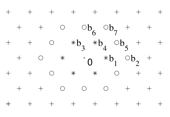
where the planar bonds $b_{i}$ are displayed in Figure 2. The remaining interaction potentials, ${\phi}_{b}(r)$ for $b\in{\mathcal{R}},$ can be obtained by symmetry from ${{\phi}}_{b_{1}}(r)={{\phi}}_{b_{6}}(r)={{\phi}}_{b_{7}}(r),$ ${{\phi}}_{b_{2}}(r),$ ${{\phi}}_{b_{4}}(r),$ and ${{\phi}}_{b_{5}}(r).$ We note that the lattice constant $a$ is contained in the definition given in the previous paragraph for the coordinates $\langle\nu_{1},\nu_{2}\rangle.$

Now observe that for $u\in\mathcal{V}$ we have $\delta\mathcal{E}^{a}(u)\in\mathcal{V}$ where the gradient $\delta\mathcal{E}^{a}(u)$ is defined by (2.5). Therefore, if a gradient-based minimization algorithm (such as the steepest descent method or the nonlinear conjugate gradient algorithm discussed below) is started from a plane displacement, it will terminate at a plane displacement. Thus, since we will only consider initial configurations which are plane displacements, we will be able to use the restriction of $\mathcal{E}^{a}$ to $\mathcal{V}\cap{\rm Adm}({u}_{0})$ in our numerical experiments. This is important since $\mathcal{E}^{a}$ restricted to $\mathcal{V}\cap{\rm Adm}({u}_{0})$ is the energy of a two dimensional crystal, and in that case the patch-test consistent atomistic to continuum coupling method developed in [37] can be used.

2.2. Energy-based quasicontinuum approximations

We will construct a local approximation to the energy $\mathcal{E}^{a}$. Our methods follow [40]. First, we define an extrapolated difference operator $\bar{D}$. The difference operator $\bar{D}$ will approximate the vector pointing from an atom to one of its neighbors using only the vectors pointing from an atom to its nearest neighbors. The nearest neighbors are the atoms depicted in Figure 2. Recall that ${\mathcal{R}}:={P}{\mathcal{M}}$; we thus have $b_{i}\in{\mathcal{R}}$ for the vectors $b_{i}$, $i=1,\dots,7$, depicted in Figure 2, and moreover, ${\mathcal{R}}$ is obtained by applying the lattice symmetries of ${\mathcal{T}}$ to $b_{1},\dots,b_{7}$. For these vectors, we define the operators

$$\bar{D}_{b_{i}}: =D_{b_{i}}\text{ for }i\in\{1,3,4\},$$

$$\bar{D}_{b_{2}}: =2D_{b_{1}},$$

$$\bar{D}_{b_{5}}: =D_{b_{1}}+D_{b_{4}},$$

$$\bar{D}_{b_{6}}: =D_{b_{3}}+D_{b_{5}},$$

$$\bar{D}_{b_{7}}: =2D_{b_{4}},$$

and extend the definition by symmetries of ${\mathcal{T}}$ so that $\bar{D}_{b}$ is defined for all $b\in{\mathcal{R}}$.

Figure 2. In the above display of the ${\hkl(1-10)}$ plane, the origin is marked with a dot, the nearest neighbors of the origin are marked with asterisks, and the other neighbors are marked with circles. The bond vector $b_{i}$ is the vector pointing from the origin to the atom marked $b_{i}$.

Using the difference operator $\bar{D}$, we define the Cauchy–Born energy by

$$\mathcal{E}^{cb}(u):={\textstyle\frac{1}{2}}\sum_{x\in{\omega}}\sum_{b\in{\mathcal{R}}_{x}}{\phi}_{b}(|b+\bar{D}_{b}u(x)|).$$

We will call the inner sum

$$\mathcal{E}^{cb}_{x}(u):={\textstyle\frac{1}{2}}\sum_{b\in{\mathcal{R}}_{x}}{\phi}_{b}(|b+\bar{D}_{b}u(x)|)$$

the continuum energy at x, so

$$\mathcal{E}^{cb}(u)=\sum_{x\in{\omega}}\mathcal{E}^{cb}_{x}(u).$$

The following remark gives a more detailed motivation for these definitions.

Remark 2.1 (The Cauchy–Born Approximation).

We call $\mathcal{E}^{cb}(u)$ the Cauchy–Born energy since, if the displacement $u$ is interpreted as a piecewise linear spline with respect to the canonical triangulation of ${\mathcal{T}}$, it can be rewritten as an integral over a stored energy density.

To make this precise, we observe that the continuum energy at $x\in{\omega}$ such that $x+b\in{\omega}$ for all $b\in{\mathcal{R}}$ is given for uniform displacements $u^{F}(x):=Fx-x$ where $F\in\mathbb{R}^{2\times 2}$ by

$$\mathcal{E}^{cb}_{x}\big{(}u^{F}\big{)}={\textstyle\frac{1}{2}}\sum_{b\in{\mathcal{R}}}{\phi}_{b}(|Fb|).$$

We thus define the Cauchy–Born stored energy density, $W_{cb}:\mathbb{R}^{2\times 2}\to\mathbb{R}\cup\{+\infty\}$, by

$$W_{cb}(F)=\frac{{\textstyle\frac{1}{2}}\sum_{b\in{\mathcal{R}}}{\phi}_{b}(|Fb|)}{v},$$

where $v$ is the area associated with each atom (in the 2D lattice). Moreover, for $u\in\mathcal{U}$, let $\bar{u}$ denote the piecewise affine interpolant of $u$ with respect to the canonical triangulation of ${\mathcal{T}}$, let $\nabla\bar{u}$ denote the resulting displacement gradient, and let $\bar{\omega}$ denote the union of those elements.

For periodic boundary conditions, or by modifying the functional $\mathcal{E}^{cb}(u)$ at the boundary $\Gamma$ of the domain ${\omega},$ one can use Shapeev’s bond density lemma [37] to prove that

$$\mathcal{E}^{cb}(u)=\int_{\bar{\omega}}W_{cb}(\nabla\bar{u})\,{\rm dx}.$$

We note that this modification of the functional $\mathcal{E}^{cb}(u)$ at the boundary does not affect the minimization of quasicontinuum energies whose set of admissible displacements, ${\rm Adm}({u}_{0}),$ are constrained in the entire boundary of ${\omega},$ such as for the Lomer Dislocation Dipole problem that we study. More detailed discussions and analyses of the Cauchy–Born approximation can be found in [18, 4, 17].

Now let ${\omega}:=\mathcal{A}\cup\mathcal{C}$ be a partition of ${\omega}$ into an atomistic region $\mathcal{A}$ and a continuum region $\mathcal{C}$. We define the energy based quasicontinuum (QCE) energy by

$$\mathcal{E}^{qce}(u):=\sum_{x\in{\mathcal{A}}}\mathcal{E}^{a}_{x}(u)+\sum_{x\in{\mathcal{C}}}\mathcal{E}^{cb}_{x}(u).$$ (2.8)

Following [40], we also define the quasi-nonlocal (QNL) energy by

$$\mathcal{E}^{qnl}(u):={\textstyle\frac{1}{2}}\sum_{x\in{\omega}}\sum_{b\in{\mathcal{R}}_{x}}\chi_{b}(x){\phi}_{b}(|b+\bar{D}_{b}u(x)|)+\left(1-\chi_{b}(x)\right){\phi}_{b}(|b+D_{b}u(x)|),$$ (2.9)

where

$$\chi_{b}(x):=\left\{\begin{array}[]{ll}1&\quad\text{ if }x\in{\mathcal{C}}\text{ and }x+b\in{\mathcal{C}},\\ 0&\quad\text{ otherwise.}\end{array}\right.$$

The reason for the introduction of the QNL method was that the QCE method did not pass the patch test [38, 11], that is, the coupling mechanism defined in (2.8) results in non-zero forces (the “ghost forces”) at the atomistic/continuum interface under homogeneous displacements (or, deformations). By contrast, it was shown in [40] that the QNL energy (2.9) does pass the patch test [40, 11, 14], as long as two atoms interact only when they share a common nearest neighbor. The authors of [40] consider only the case where the pair potential does not depend on the bond direction. Nonetheless, the argument which they give may be applied to show that the QNL energy (2.9) passes the patch test also in the present case.

The importance of passing the patch test lies in the fact that the “ghost forces” can be understood as a consistency error, which results in an $O(1)$ relative error in the displacement gradient [11]. Moreover, it was shown in [14], that they can result in a $O(1)$ relative error in the prediction of critical loads at which lattice instabilities occur.

To achieve an efficient quasicontinuum method, the positions of atoms in the continuum region are normally further constrained by piecewise linear interpolation [30]. The development of an implementable and patch-test consistent quasicontinuum energy that allows coarsening by piecewise linear interpolation in the continuum region has been achieved so far only for two-dimensional problems with pair potential interactions [37]. The development of patch-test consistent quasicontinuum energies for many-body potentials such as the popular embedded atom method (EAM) or for three-dimensional problems is an open problem.

2.3. The force based quasicontinuum approximation

The force based quasicontinuum (QCF) approximation gives a patch-test consistent approximation for atomistic-to-continuum coupling even with coarsening in the continuum region [6, 8]. Force-based multiphysics coupling methods are generally popular because of their algorithmic simplicity. However, force-based coupling methods are known to give non-conservative force fields [6, 8], and our recent research described at the end of this section has discovered additional stability problems for QCF approximations and solution methods [15].

Instead of approximating the energy $\mathcal{E}^{a}$ by a local energy, we can approximate the forces ${\mathcal{F}}(u)$ directly. This leads to the force based quasicontinuum (QCF) approximation. As above, let ${\omega}:=\mathcal{A}\cup\mathcal{C}$ be a partition of ${\omega}$ into an atomistic region $\mathcal{A}$ and a continuum region $\mathcal{C}$. Define ${\mathcal{F}}^{qcf}:\mathcal{V}\rightarrow\mathcal{V}$ by

$${\mathcal{F}}^{qcf}(u)(x):=\left\{\begin{array}[]{ll}-\delta\mathcal{E}^{a}(u)(x)&\quad\text{ if }x\in\mathcal{A},\\ -\delta\mathcal{E}^{cb}(u)(x)&\quad\text{ if }x\in\mathcal{C}.\end{array}\right.$$ (2.10)

We consider the boundary value problem

$${\mathcal{F}}^{qcf}(u)(x) =0 \quad\text{ for all }x\in{\omega}\setminus\Gamma,$$ (2.11)

$$u(x) =u_{0}(x) \quad\text{ for all }x\in\Gamma.$$

It was shown in [13, 12, 28], for one-dimensional model problems, that the solution of problem (2.11) approximates the solution of problem (2.6). It is also true that the QCF method passes the patch test [8].

In our numerical experiments we will solve equation (2.11) using an iterative method defined in [8, 9]. Let $u_{0}\in\mathcal{V}$ be given, and let $\mathcal{E}^{qc}$ be either $\mathcal{E}^{qnl}$ or $\mathcal{E}^{qce}$. Then we let $u_{n+1}\in{\rm Adm}({u}_{0})\cap\mathcal{V}$ be the solution of the problem:

$$u_{n+1}\in\operatorname*{arg\ local\ min}_{v\in{\rm Adm}({u}_{0})\cap\mathcal{V}}\left\{\mathcal{E}^{qc}(v)-\sum_{x\in{\omega}}\left({\mathcal{F}}^{qcf}(u_{n})(x)+\delta\mathcal{E}^{qc}(u_{n})(x)\right)\cdot v(x)\right\}.$$ (2.12)

The method (2.12) with $\mathcal{E}^{qc}=\mathcal{E}^{qce}$ is the popular ghost force correction method proposed in [30]. We have proposed the method $\mathcal{E}^{qc}=\mathcal{E}^{qnl}$ as a ghost force correction method with improved stability properties [15]. For $\mathcal{E}^{qc}=\mathcal{E}^{qce},$ we call the iteration (2.12) the QCF-QCE iteration; for $\mathcal{E}^{qc}=\mathcal{E}^{qnl},$ we call it the QCF-QNL iteration.

The Euler–Lagrange equation for problem (2.12) is

$$\delta\mathcal{E}^{qc}(u_{n+1})(x) ={\mathcal{F}}^{qcf}(u_{n})(x)+\delta\mathcal{E}^{qc}(u_{n})(x) \quad\text{ for all }x\in{\omega}\setminus\Gamma,$$

$$u_{n+1}(x) =u_{0}(x) \quad\text{ for all }x\in\Gamma.$$

It is easy to see that, if the sequence of iterates converges, then its limit must be a solution of problem (2.11). Moreover, under certain technical conditions related to the stability of the preconditioner $\mathcal{E}^{qc},$ it can be shown that the sequence indeed converges [8, 9, 15].

A QCF solution method that can theoretically give inaccurate results is the use of a nonlinear conjugate gradient solver for the force-based quasicontinuum equations [31, 39, 6]. We have proven that the linearization of the force-based equilibrium equations is not positive definite [13], which implies that the conjugate gradient solution of this problem is unstable [15]. We have discovered from informal discussions with computational physicists that their conjugate gradient iterative solution of force-based multiphysics coupling methods sometimes oscillates rather than converges, a phenomenon partially explained by our theoretical analysis of this instability. We are developing benchmark tests to further study the reliability of the conjugate gradient solution of the force-based quasicontinuum equations.

We have shown theoretically and computationally for one-dimensional model problems that the GMRES method is a reliable and efficient solver for the force-based quasicontinuum equations [15]. We are thus also preparing multi-dimensional benchmark tests to evaluate the reliability and efficiency of the GMRES solution of the force-based quasicontinuum equations.

3. Numerical Experiments

3.1. The Lomer Dislocation Dipole: Analytical Model

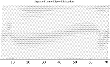
Following the numerical experiments presented in [31], we consider a dipole of Lomer dislocations, as depicted in Figure 3. The Lomer dislocation has Burgers vector $b=\hkl[110]$ in the $\hkl(001)$ plane [20]. The dipole should be a stable equilibrium if the distance between the cores is large enough so that the Peach-Koehler elastic attraction of the dislocations is weaker than the critical force needed to overcome the Peierls energy barrier [31].

Figure 3. The atomistic and continuum (yellow) domains for the Lomer dislocation dipole. The size of the total computational domain is $L_{1}=75\times a/\sqrt{2}$ and $L_{2}=60\times a$ where $a$ is the length of the sides of the cubic supercell. The atomistic domain is given by $D_{1}=k\times a/\sqrt{2}$ and $D_{2}=k\times a$ for $k=3,\,4,\,5.$ The separation of the dipole used in the initial guess $u_{elas}$ is $w=10\times a/\sqrt{2}.$

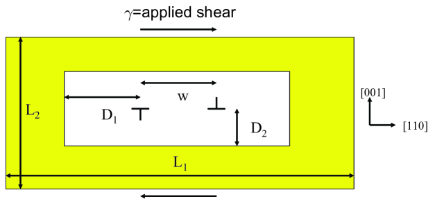
We will study the stability of the dipole when a shear is applied to the crystal. By a shear, we mean a homogeneous deformation of the lattice ${\mathcal{T}}$ that takes the form

$$x\mapsto\sigma(\gamma)x\quad\text{where}\quad\sigma(\gamma):=\left(\begin{array}[]{cc}1&\gamma\\ 0&1\end{array}\right).$$

We call $\gamma$ the shear strain. We say that the shear is positive if $\gamma>0$ and negative if $\gamma<0$. More generally, we will apply a shear to the deformation $x+u(x)$ given by the displacement $u(x)$ to obtain the sheared deformation

$$x+u(x)\mapsto\sigma(\gamma)\left(x+u(x)\right).$$

A positive shear applied to the top and bottom boundaries of the crystal changes the energy landscape to favor the movement of the dislocations apart. As $\gamma$ increases, the shear force overwhelms both the Peierls force and the Peach-Koehler elastic attraction. Thus, the original equilibrium configuration of the dipole becomes unstable, and the dislocations move away from each other. We call the value of $\gamma$ at which this instability occurs the critical strain. In our numerical experiments, we will simulate the process of slowly shearing the crystal until the critical strain is reached.

To understand the movement of the Lomer dipole theoretically, we model the local minima of the atomistic energy for displacements constrained on the boundary $\Gamma$ to be $\sigma(\gamma)x-x$ and constrained to be in the energy well of a Lomer dipole with separation $w:$

$$\inf_{v\in\widetilde{{\rm Adm}}\left(\sigma(\gamma)x-x,\,w\right)}\mathcal{E}^{a}(v)\approx \tilde{\mathcal{E}}^{a}(w,\gamma)=\mathcal{E}^{a}_{\text{misfit}}(w)+\mathcal{E}^{a}_{\text{dipole attraction}}(w)$$

$$+\mathcal{E}^{a}_{\text{applied shear}}(w,\gamma)+\mathcal{E}^{a}_{\text{boundary effect}}(w,\gamma)$$

where $\widetilde{{\rm Adm}}\left(\sigma(\gamma)x-x,\,w\right)$ is the set of admissible displacements roughly described above. Here the classical Peierls-Nabarro misfit energy [20], the classical Peach-Koehler interaction energy [20], and our modeling of the effect of the applied shear are given for $w\geq 0$ and $\gamma\geq 0$ by

$$\begin{split}&\mathcal{E}^{a}_{\text{misfit}}(w)=\frac{\mu b}{2\pi(1-\nu)}\cos\frac{2\pi w}{b}\exp\left[{-\frac{\pi d}{(1-\nu)b}}\right],\\ &\mathcal{E}^{a}_{\text{dipole attraction}}(w)=\frac{\mu b^{2}}{2\pi}\ln\frac{w}{L},\\ &\mathcal{E}^{a}_{\text{applied shear}}(w,\gamma)=\beta_{1}w+\beta_{2}\gamma-\frac{\beta_{3}\gamma\,w}{L},\end{split}$$ (3.1)

where $\mu$ is a characteristic shear modulus, $\nu$ is a characteristic Poisson’s ratio, $L$ is a characteristic length, $b=a/\sqrt{2}$ is the magnitude of the Burger’s vector, $d=a/\sqrt{2}$ is the interatomic spacing between the ${\hkl(1-10)}$ planes, and $\beta_{1},\ \beta_{2}$ and $\beta_{3}$ are constants with $\beta_{3}>0.$ Although our model for the misfit energy $\mathcal{E}^{a}_{\text{misfit}}(w)$ and the dipole attraction $\mathcal{E}^{a}_{\text{dipole attraction}}(w)$ are well-known approximations of the atomistic energy $\mathcal{E}^{a}(v)$ [20], our bilinear model for the shear energy $\mathcal{E}^{a}_{\text{shear}}(w,\gamma)$ is not derived from the atomistic energy and our justification is based only on the qualitative behavior it predicts for the stability of the Lomer dipole.

After scaling the atomistic energy $\mathcal{E}^{a}(v),$ the dipole separation $w,$ and the shear strain $\gamma,$ and after neglecting the boundary effect $\mathcal{E}^{a}_{\text{boundary effect}}(w,\gamma)=0,$ we can obtain from (3.1) the model

$$\tilde{\mathcal{E}}^{a}(w,\gamma)=\cos w+\beta\ln w-\gamma w$$ (3.2)

for some $\beta>0.$ We chose $\beta=12$ in our numerical experiments. We then find that the force conjugate to the dipole separation $w$ is given by

$$-\frac{\partial\tilde{\mathcal{E}}^{a}(w,\gamma)}{\partial w}=\sin w-\frac{\beta}{w}+\gamma.$$ (3.3)

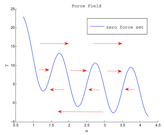
We can see from the force field displayed in Figure 4 that the dipole separation $w$ becomes unstable at a critical shear strain $\gamma$ and will tend to infinity under gradient flow dynamics for the force field  (3.3) (for example, consider the stability of the equilibrium solution branch starting at $w=1.5$ as $\gamma$ is increased). The Lomer dislocations similarly separated to the boundary at a critical shear strain $\gamma$ in our numerical experiments (see Figure 5).

Figure 4. The force field  (3.3) for the Lomer dipole model (3.2) with $\beta=12.$

Figure 5. Separation of the Lomer dislocations to the boundary after continuation past a critical strain to $\gamma=0.070.$ Cartensian coordinates are used to label the axes. The top and bottom of the deformation of the reference domain ${\omega}$ are not displayed, but the entire width of the deformed reference domain is displayed. The triangular mesh was constructed from the reference lattice.

3.2. The Lomer Dislocation Dipole: Numerical Experiments

In out numerical experiments we use the Morse interatomic potential

$$\phi(r):=\left(1-\exp(\alpha(r-1))\right)^{2}\quad\text{for }r>0,$$

with

$$\alpha:=4.4.$$

We remark that we did not choose $\alpha=4.4$ in order to model some specific material. Rather, we chose this value of $\alpha$ as small as possible while retaining a stable dipole. For smaller values of $\alpha$ we were unable to compute a stable dipole, whereas, if $\alpha$ is chosen too large then the atomistic, Cauchy–Born, and quasicontinuum models are almost identical since the first neighbor interactions, which would become dominant, are treated identically in all models.

We chose the lattice spacing $a$ so that the FCC lattice $\mathcal{L}$ is a ground state for the atomistic energy defined by the Morse potential and using a cut-off radius that includes first, second, third, and fourth-nearest neighbor interactions (determined from the reference positions). Specifically, we let $a$ be the minimizer of

$$\psi(r):=12\phi\left(\sqrt{\frac{1}{2}}r\right)+6\phi\left(r\right)+24\phi\left(\sqrt{\frac{3}{2}}r\right)+12\phi\left(\sqrt{2}r\right),$$

which is the energy per atom in the undeformed lattice with lattice spacing $r$ since each atom in the ${\mathcal{L}}$ lattice has $12$ nearest neighbors, $6$ next-nearest neighbors, $24$ third-nearest neighbors, and $12$ fourth-nearest neighbors (see (2.3)). The minimum is attained when $a=1.3338$.

We let ${\omega}$ be the rectangular domain consisting of $150$ columns of atoms parallel to $V_{2}$ with each column containing $60$ atoms defined in the $\langle\nu_{1},\,\nu_{2}\rangle$ coordinates by

$$\begin{split}{\omega}&=\left\{\langle k,\,l\rangle:0\leq k\leq 74,\ 0\leq l\leq 59\right\}\\ &\qquad\qquad\cup\left\{\langle k+1/2,\,l+1/2\rangle:0\leq k\leq 74,\ 0\leq l\leq 59\right\}.\end{split}$$

We take the boundary $\Gamma$ of ${\omega}$ to be a layer of atoms four rows deep around the edges of ${\omega},$ so that

$$\begin{split}\Gamma&=\left\{\langle k,\,l\rangle:k=0,\,1,\,73,\,74,\ 0\leq l\leq 59\right\}\\ &\qquad\qquad\cup\left\{\langle k+1/2,\,l+1/2\rangle:k=0,\,1,\,73,\,74,\ 0\leq l\leq 59\right\}\\ &\qquad\qquad\cup\left\{\langle k+1/2,\,l+1/2\rangle:0\leq k\leq 74,\ l=0,\,1,\,58,\,59\right\}\\ &\qquad\qquad\cup\left\{\langle k+1/2,\,l+1/2\rangle:0\leq k\leq 74,\ l=0,\,1,\,58,\,59\right\}.\end{split}$$

With this choice of $\Gamma$, for any atom $x\in{\omega}\setminus\Gamma$, all fourth-neighbors of $x$ belong to ${\omega}$. Thus, there are no boundary effects for the reference lattice when $a=1.3338.$ This choice of $\Gamma$ corresponds to taking Dirichlet boundary conditions on the entire boundary. Throughout the rest of this section, we will consider only displacements $u$ so that for some $\gamma>0$, we have $u(x)=\sigma(\gamma)x-x$ for all $x\in\Gamma$. For such a displacement, we will call the shear strain $\gamma$ the shear on the boundary.

We will now discuss how the stable Lomer dipoles displayed in Figure 6 are computed. We first construct an initial guess $u_{elas}$ for the displacement field corresponding to a Lomer dipole by using the displacement fields of the isotropic, linear elastic solution for the edge dislocations [20] at the left and right pole of the dipole, respectively. More precisely, the formula for these displacement fields is

$$u_{1}^{*}= \frac{b^{*}}{2\pi}\Bigg{[}\tan^{-1}\frac{x_{2}-x_{2}^{*}}{x_{1}-x_{1}^{*}}+\frac{(x_{1}-x_{1}^{*})(x_{2}-x_{2}*)}{2(1-\nu)\Big{(}(x_{1}-x_{1}^{*})^{2}+(x_{2}-x_{2}^{*})^{2}\Big{)}}\Bigg{]},$$

$$u_{2}^{*}= -\frac{b^{*}}{2\pi}\Bigg{[}\frac{1-2\nu}{4(1-\nu)}\ln\Big{(}x_{1}-x_{1}^{*})^{2}+(x_{2}-x_{2}^{*})^{2}\Big{)}$$

$$\qquad\qquad+\frac{(x_{1}-x_{1}^{*})^{2}-(x_{2}-x_{2}^{*})^{2}}{4(1-\nu)\Big{(}(x_{1}-x_{1}^{*})^{2}+(x_{2}-x_{2}^{*})^{2}\Big{)}}\Bigg{]},$$

where $*=L,R$ refers to the left or the right edge dislocation, respectively, $b^{*}$ is the corresponding Burgers vector, and $x_{i}^{*}$, $i=1,2$, are the components of the position vectors [20]. In our numerical experiments, we set the initial positions of the Lomer dislocations in the reference configuration to be (in the $\langle\nu_{1},\,\nu_{2}\rangle$ coordinates)

$$\left\langle\nu_{1}^{L},\nu_{2}^{L}\right\rangle=\left\langle 32,30+\frac{1}{6}\right\rangle\quad\text{and}\quad\left\langle\nu_{1}^{R},\nu_{2}^{R}\right\rangle=\left\langle 42,30+\frac{1}{3}\right\rangle.$$

We note that initial dislocation positions are placed between the center row of atoms at $\nu_{2}=30$ and the first row above the center $\nu_{2}=30+1/2,$ with $\nu_{2}^{L}=30+1/6$ and $\nu_{2}^{R}=30+1/3$ placed symmetrically about $\nu_{2}=30+1/4$ (see Figure 6).

The displacements $u^{L},u^{R}$, are estimates of the displacement fields for isolated edge dislocations. By superimposing them, we obtain an estimate of the elastic displacement field for the dipole (without shear):

$$u_{elas}=u^{L}+u^{R}.$$

Finally, we apply a shear deformation to the deformation field $x+u_{elas}$,

$$x+u^{0}_{elas}(x)=\sigma(\gamma)\left(x+u_{elas}(x)\right),$$

which yields an initial guess for the displacement field for the Lomer dipole under applied shear:

$$u^{0}_{elas}(x)=\sigma(\gamma)\left(x+u_{elas}(x)\right)-x.$$

We use the displacement $u_{elas}^{0}=\sigma(\gamma_{0})u_{elas}(x)-x$ as a starting guess for a preconditioned nonlinear conjugate gradient method (P-nCG), which is described in Section 5, to solve the minimization problem (2.6).

It is challenging to find a stable dipole. In fact, we were unable to find a stable dipole without applying a positive shear to the boundary. That is, we did not find a Lomer dipole that was a local minimum of the atomistic energy (2.7) subject to the boundary condition $u(x)=0$ for all $x\in\Gamma$. We were also unable to find a stable dipole when the parameter $\alpha$ in the Morse potential was too small. Essentially, we found that as $\alpha$ decreased, the interval of shear strains for which a given dipole was stable became smaller. After some experimentation, we did find a stable Lomer dipole with $\alpha=4.4$ and with shear on the boundary $\gamma_{0}=0.0375$.

Our atomistic and quasicontinuum models utilize a fourth-nearest neighbor cutoff calculated from the positions in the reference lattice, which is in fact the largest possible neighborhood for the QNL method applied to an FCC lattice [40]. Such a cutoff is acceptable for atomistic configurations that are “close” to the reference lattice, however, for the highly deformed positions near the dipole a cutoff in deformed coordinates ought to be used. Even though the dominant nearest-neighbour interactions are always included in our calculation, a more precise understanding of the error committed for second- to fourth-nearest neighbours is required.

Next we describe how we simulate the shearing of the dipole. For simplicity, we will explain how this is done for energy-based methods before we discuss the force-based method. Let $u_{0}$ be the displacement field of the stable Lomer dipole discussed above. Suppose that $\gamma_{0}$ is the shear on the boundary for $u_{0}$. Let $\gamma_{k}$ be an increasing sequence of shear strains, and let $\delta\gamma_{k+1}:=\gamma_{k+1}-\gamma_{k}$. $\mathcal{E}$ can be either the atomistic energy (2.7), the QCE energy (2.8), or the QNL energy (2.9).

We perform the following iteration starting with the displacement $u_{0}$. Suppose we have a dipole with displacement field $u_{k}$ which solves the boundary value problem

$$\mathcal{-\delta\mathcal{E}}(u_{k})(x) =0 \quad\mbox{ for all }x\in{\omega}\setminus\Gamma,$$

$$u_{k}(x) =\sigma(\gamma_{k})x-x \quad\mbox{ for all }x\in\Gamma.$$

We let

$$u^{0}_{k+1}(x)=\sigma(\delta\gamma_{k})\left(x+u_{k}(x)\right)-x.$$

Observe that $u^{0}_{k+1}$ satisfies the boundary condition

$$u^{0}_{k+1}(x)=\sigma(\gamma_{k+1})x-x\quad\mbox{ for all }x\in\Gamma.$$

We use the P-nCG algorithm to compute a new local minimizer $u_{k+1}$ “near” $u^{0}_{k+1}$, which satisfies the new boundary condition $u_{k+1}(x)=\sigma(\gamma_{k+1})x-x$ for all $x\in\Gamma$. We call this process the shear loading continuation.

We terminate the shear loading continuation when we can no longer find an equilibrium $u_{k+1}(x)$ close to the initial guess $\sigma(\delta\gamma_{k+1})\left(x+u_{k}(x)\right)-x.$ In practice, this means that we stop when the nCG algorithm returns a deformation in which the cores of the dislocations have moved apart. If the dislocations move apart at the $(k+1)^{th}$ step of the iteration, then we assume that the critical strain must be between $\gamma_{k}$ and $\gamma_{k+1}$.

For the force based approximation (2.10), we use a similar iteration to find the critical strain. At each step in the iteration, we solve the boundary value problem

$$\mathcal{F}^{qcf}(u_{k+1})(x) =0 \quad\mbox{ for all }x\in{\omega}\setminus\Gamma,$$ (3.4)

$$u_{k+1}(x) =\sigma(\gamma_{k+1})x-x \quad\mbox{ for all }x\in\Gamma.$$

We solve equation (3.4) using the ghost force correction iteration defined in equation (2.12). We use the same initial guess

$$u^{0}_{k+1}(x):=\sigma(\delta\gamma_{k+1})\left(x+u_{k}(x)\right)-x$$

as in the energy-based case, and we solve each iteration of ghost force correction using the P-nCG algorithm.

We presented computational results for the deformation of a Lennard-Jones chain under tension in [9] that demonstrate the necessity of using a sufficiently small parameter step size to ensure that the computed solution remains in the domain of convergence of the ghost force correction iteration (defined below as QCE-QCF) method. These results exhibit fracture before the actual load limit if the parameter step size is too large. We thus conclude that the shear strain $\delta\gamma_{k+1}$ must be sufficiently small to ensure that our computed solution remains in the domain of convergence of the QCE-QCF method since it would otherwise predict instability for the Lomer dipole before that predicted by the QCF method.

We perform the shear loading iteration for each of the quasicontinuum methods using three different atomistic regions, as depicted in Figure 6. The atomistic region (3) (resp., (4), (5)) is a box containing the dipole such that there are three (resp., four, five) rows of atoms between the continuum region and each of the atoms in the pentagons surrounding the cores of the dislocations, or more precisely, the atomistic region ($k$) is the box given in $\langle\,\nu_{1},\,\nu_{2}\,\rangle$ coordinates by $[32-k,43+k]\times[30-k,30+k]$ for $k=3,4,5$. Throughout the remainder of this section, QNL-QCF (resp. QCE-QCF) will refer to the QCF method implemented using the ghost force correction iteration preconditioned by the QNL (resp. QCE) energy [15]. We will let QNL-QCF(k) (resp. QCE-QCF(k), QNL(k), QCE(k)) refer to the QNL-QCF (resp. QCE-QCF, QNL, QCE) method with atomistic region (k) for k one of $3,\ 4,\text{ or }5.$

(a) Atomistic region (3)

(b) Atomistic region (4)

(c) Atomistic region (5)

Figure 6. The atomistic regions for the Lomer dislocation dipole. Not all of the continuum region is displayed. The mesh is the Delaunay triangulation [7] of the reference lattice (i.e., with the atoms as the nodes). The atomistic region is shaded grey.

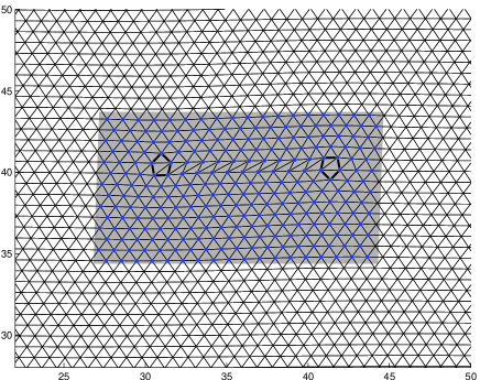
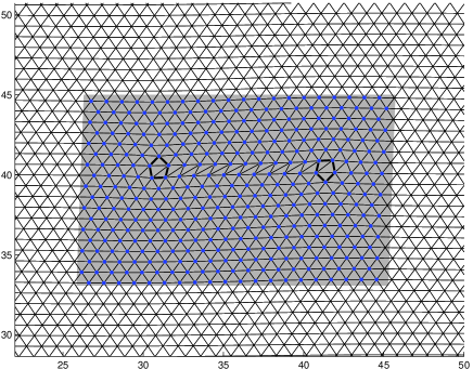
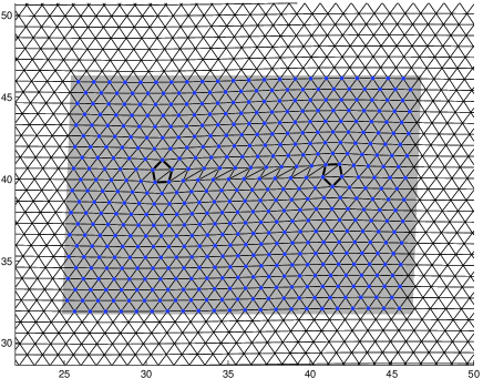
We note that the atomistic regions studied in the benchmark tests given in [31] extended to the lateral boundaries of the computational domain ${\omega},$ or, following the notation used in Figure 3 these tests study the case $2D_{1}+w=L_{1}.$ Thus, the benchmark tests [31] do not present the capture of a Lomer dipole in an atomistic region fully surrounded by a continuuum region and do not study the effect of coupling error in the dipole plane $\hkl(110).$

In Table 1, we give the critical strains for each method in decreasing order. The columns $\gamma^{-}$ and $\gamma^{+}$ are the shear strains at the last step before the dislocations moved apart, and at the first step for which the dislocations moved, respectively. The column labeled “Error” displays the relative error from the critical strain of the atomistic model, calculated by the formula

$$\text{Error}=\frac{\bar{\gamma}_{at}-\bar{\gamma}_{qc}}{\bar{\gamma}_{at}},$$ (3.5)

where $\bar{\gamma}_{at}$ is the mean of $\gamma^{-}$ and $\gamma^{+}$ for the atomistic method, and $\bar{\gamma}_{qc}$ is the mean of $\gamma^{-}$ and $\gamma^{+}$ for the quasicontinuum method. We wish to stress that if $\gamma^{+}$ for some method is equal to $\gamma^{-}$ for another method, then no strong statement can be made comparing critical strains of the two methods. For example, our data do not show that QNL(5) has a significantly higher critical strain than QCE-QCF(5). Rather, our data suggest only that the critical strain of the QCE-QCF(5) method is in the interval $[0.038172,0.038177]$ and that the critical strain of the QNL(5) method is in $[0.038177,0.038181]$. Thus, the critical strains of the two methods are very close.

The reader will observe that the critical strain of the fully atomistic model is the highest. The critical strain predicted by the QCE method is the lowest, and is the farthest from the critical strain of the atomistic model. This is not surprising in light of the results on the stability of one dimensional chains obtained in  [14]. It is surprising, however, that the QNL method predicts the critical strain of the atomistic model more accurately than the QNL-QCF force-based method, since we expected that the stability of the QNL-QCF method would be determined by the QNL preconditioner [15]. It also somewhat surprising that the QCE-QCF iteration predicted the critical strain as accurately as the QNL-QCF iteration. The analysis given in  [15] suggests that the QCE-QCF iteration should lose stability at a lower strain than the QNL-QCF iteration.

Table 1. The critical strain for the Lomer dislocation dipole under shear. The Error is given by $\left(\bar{\gamma}_{at}-\bar{\gamma}_{qc}\right)/{\bar{\gamma}_{at}}$ in percent which is defined precisely in the paragraph surrounding (3.5).

Method	Critical Strain		Error
	$\gamma^{-}$	$\gamma^{+}$
Atomistic	0.038190	0.038194	0.000 %
QNL(5)	0.038177	0.038181	0.034 %
QCE-QCF(5)	0.038172	0.038177	0.046 %
QNL-QCF(5)	0.038172	0.038177	0.046 %
QNL(4)	0.038164	0.038168	0.069 %
QCE-QCF(4)	0.038155	0.038159	0.092 %
QNL-QCF(4)	0.038155	0.038159	0.092 %
QNL(3)	0.038111	0.038116	0.206 %
QCE-QCF(3)	0.038081	0.038085	0.286 %
QNL-QCF(3)	0.038081	0.038085	0.286 %
QCE(3)	0.037750	0.037775	1.125 %

Figure 7 consists of graphs showing the relative $w^{1,\infty}$ error versus the shear strain for various quasicontinuum methods. The $w^{1,\infty}$ norm is defined by

$$||u||_{w^{1,\infty}}:=\max_{x\in{\omega}}\max_{b\in\mathcal{N}_{x}}\frac{|D_{b}u(x)|}{|b|},$$

and we define the relative error in $w^{1,\infty}$ by

$$\rm{err_{rel}}(u_{qc},u_{a}):=\frac{||u_{qc}-u_{a}||_{w^{1,\infty}}}{||u_{a}||_{w^{1,\infty}}}.$$ (3.6)

Here $u_{qc}$ denotes a solution of one of the quasicontinuum models, and $u_{a}$ denotes a solution of the atomistic model with the same boundary conditions.

The reader will observe that the error of the QCE method is the greatest. This is largely due to the presence of ghost forces [10]. The error of the QNL method is the least. Again, this is surprising since various analyses  [11, 34, 15, 13, 28] suggest that the force based method should be more accurate than the QNL method. However, we note that a similar effect was observed in one-dimensional numerical experiments in [28]: while for large atomistic regions the QCF method was considerably more accurate than the QNL method, for smaller atomistic regions the QNL method was clearly more accurate. The atomistic regions studied here in our numerical experiments for the Lomer dislocation dipole are very small.

Figure 7. The relative error $\rm{err_{rel}}(u_{qc},u_{a})=||u_{qc}-u_{a}||_{w^{1,\infty}}/||u_{a}||_{w^{1,\infty}}$ in $w^{1,\infty}$ for the Lomer dislocation dipole.

3.3. Tensile Loading

In our next experiment, we examine the accuracy of various quasicontinuum methods for the computation of the resistance to slip under an applied tension. By a tension, we mean a homogeneous deformation of the lattice ${\mathcal{T}}$ which takes the form

$$x\mapsto\tau(\gamma)x\quad\text{where}\quad\tau(\gamma):=\left(\begin{array}[]{cc}1+\gamma&0\\ 0&1\end{array}\right)$$

when expressed in the basis of the coordinate vectors $V_{1}$ and $V_{2}$. We will let $\tau(\gamma)$ denote such a tension, and we will call $\gamma$ the tensile strain. We call a tension positive if $\gamma>0$ and negative if $\gamma<0$.

In our numerical experiments, we use the same pair potential and lattice spacing as for the Lomer dipole problem. We let ${\omega}$ be the rectangular domain consisting of $120$ columns of atoms parallel to $V_{2}$ with each column containing $15$ atoms defined in the $\langle\,\nu_{1},\,\nu_{2}\,\rangle$ coordinates by

$$\begin{split}{\omega}&=\left\{\langle k,\,l\rangle:0\leq k\leq 59,\ 0\leq l\leq 14\right\}\\ &\qquad\qquad\cup\left\{\langle k+1/2,\,l+1/2\rangle:0\leq k\leq 59,\ 0\leq l\leq 14\right\}.\end{split}$$

We will now let $\Gamma$ consist of four columns of atoms parallel to $V_{2}$ at the left edge of ${\omega}$, and four columns at the right edge of ${\omega},$ that is,

$$\begin{split}\Gamma&=\left\{\langle k,\,l\rangle:k=0,\,1,\,58,\,59,\ 0\leq l\leq 14\right\}\\ &\qquad\qquad\cup\left\{\langle k+1/2,\,l+1/2\rangle:k=0,\,1,\,58,\,59,\ 0\leq l\leq 14\right\}.\end{split}$$

This corresponds to choosing Dirichlet boundary conditions on the sides of $\omega$ parallel to $V_{2}$, and free boundary conditions on the sides of $\omega$ parallel to $V_{1}$.

To find the critical strain for the crystal under tension, we perform an iteration similar to the shear loading iteration. Let $\gamma_{k}$ be an increasing sequence of tensile strains with $\gamma_{0}=0$. We let $u_{0}$ be the displacement field of the undeformed reference lattice ${\omega}$ described above. Then we let $u_{k+1}$ solve the problem

$$\mathcal{F}(u_{k+1})(x) =0 \quad\mbox{ for all }x\in{\omega}\setminus\Gamma,$$ (3.7)

$$u_{k+1}(x) =\tau(\gamma_{k+1})x-x \quad\mbox{ for all }x\in\Gamma.$$

Here $\mathcal{F}$ is the gradient of one of the energies (2.7), (2.8),  (2.9), or else the force-based method (2.10). We solve equation (3.7) using the same methods discussed above for the shear loading iteration, except that in this case we start each step with the initial guess

$$u_{k+1}^{0}(x):=\tau\left({\textstyle\frac{1+\gamma_{k+1}}{1+\gamma_{k}}}\right)\left(x+u_{k}(x)\right)-x.$$

We call this iteration the tensile loading continuation. We stop the continuation when the P-nCG algorithm (or a ghost force correction iteration) returns a deformation in which a slip has occurred.

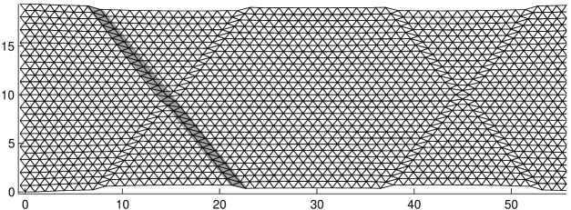
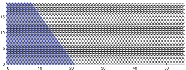
Our numerical experiments are designed to test how well the boundary between the atomistic and continuum regions resists slip under tensile loading. When we perform the tensile loading iteration for the fully atomistic model, we found that a slip tends to occur along the slip plane indicated in Figure 8(a) when a critical tensile load is reached. Figure 8(a) shows the configuration of the crystal immediately after a typical slip has occurred. We note that the slip allows the crystal to accommodate an increased tensile strain with a decrease in the energy. We then chose an atomistic region ${\mathcal{A}}$ whose boundary is along that line, as depicted in Figure 8(b).

(a) The natural slip plane. We choose an atomistic region whose boundary is the plane highlighted in grey. The mesh is the Delaunay triangulation [7] of the reference lattice.

(b) The atomistic region ${\mathcal{A}}$ is shaded grey. All atoms in ${\mathcal{A}}$ are marked with a blue dot.

Figure 8. The atomistic (${\mathcal{A}}$) and continuum ($\mathcal{C}$) regions for the tensile loading experiment.

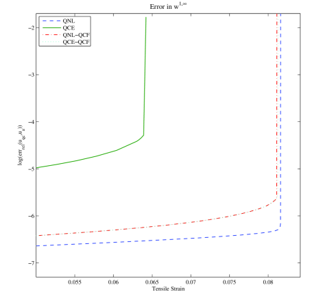
We observe that the critical strains of the quasicontinuum models were lower than the critical strain of the atomistic model. Our results are summarized in Table 2. In Table 2, the columns $\gamma^{-}$ and $\gamma^{+}$ are the tensile strains at the last step before slip is observed and at the first step for which slip is observed, respectively. The column labeled “Error” is the percent error from the critical strain of the atomistic model.

Table 2. The critical strain under tension. The Error is given by $\left(\bar{\gamma}_{at}-\bar{\gamma}_{qc}\right)/{\bar{\gamma}_{at}}$ in percent, which is defined in (3.5).

Method	Critical Strain		Error
	$\gamma^{-}$	$\gamma^{+}$
Atomistic	0.081635	0.081649	0.000 %
QNL	0.081593	0.081607	0.052 %
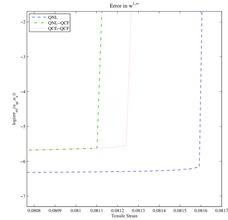
QCE-QCF	0.081242	0.081270	0.473 %
QNL-QCF	0.081101	0.081130	0.645 %
QCE	0.063900	0.064200	21.548 %

We observe that the critical strain of the QCE model is lower than the critical strain of any of the other models. This is in agreement with the one dimensional stability results established in  [14]. However, we were surprised to find that the critical strain predicted by the QNL method is higher than the critical strain predicted by the QNL-QCF force based method, since we expected that the stability of the QNL-QCF method would be determined by the QNL preconditioner [15]. We were also surprised to observe that the critical strain of the QNL-QCF method is less than the critical strain of QCE-QCF. The one-dimensional analyses in  [12, 15] suggest that the force based methods should have a comparable critical strain as QNL, and that the QCE-QCF iteration should lose stability at a lower strain than the QNL-QCF iteration.

Figure 9 consists of graphs showing the relative $w^{1,\infty}$ error versus the tensile strain for various quasicontinuum methods. We observe that the QCE model had the greatest error. This is primarily the result of the ghost forces which arise in the QCE model. The QNL model had the lowest error. Again, this is somewhat surprising in light of the one dimensional theory [11, 34, 15, 13, 28], which predicts that the force based methods should have lower error than the QNL method.

Figure 9. The relative error $\rm{err_{rel}}(u_{qc},u_{a})=||u_{qc}-u_{a}||_{w^{1,\infty}}/||u_{a}||_{w^{1,\infty}}$ in $w^{1,\infty}$ for tensile loading.

4. Conclusion

Materials scientists and engineers typically attempt to verify their multiphysics methods by benchmark tests. However, definitive conclusions from these benchmark tests are often not possible since they combine many sources of error (modeling error, coupling error, solution error, boundary condition error, etc.). Further supporting theory is needed to select a set of test problems that thoroughly samples the solution space.

We are developing an improved theoretical basis for benchmarking atomistic-to-continuum coupling methods based on the multiscale numerical analysis developed by us and others. Our goal is to be able to reliably predict the accuracy of atomistic-to-continuum coupling methods for general deformations and loads from numerical experiments for a small set of mechanics problems. This set of mechanics problems should sample the fundamental modes of material instability such as dislocation formation, slip, and fracture.

Our discussion of the benchmark tests presented in this paper give many examples of the predictive success of the theoretical analysis we have developed during the past few years, but we also describe several cases where our theoretical analysis seems to predict a different outcome than our computational experiments. This discrepancy between theory and computational experiment occurs when our theoretical analysis does not adequately model the computational problem and is motivation to develop more general theoretical analysis.

5. Appendix: A Preconditioned Conjugate Gradient Algorithm

In this appendix, we describe the preconditioned nonlinear conjugate gradient optimization algorithm (P-nCG) and the corresponding linesearch method, which we used in the numerical experiments in this paper.

Let $\mathcal{E}:\mathbb{R}^{N}\to\mathbb{R}\cup\{+\infty\}$ be continuously differentiable in $\{u:\mathcal{E}(u)<\infty\}$. If $\mathcal{E}$ is an energy of the type discussed above, then the standard nonlinear conjugate gradient method [33, Sec. 5.2] is convergent, but very inefficient, due to the poor conditioning of the Hessian matrix at local minima.

Let ${\rm P}\in\mathbb{R}^{N\times N}$ be a symmetric positive definite matrix, e.g., a discrete Laplacian or a modification thereof. A simple but considerably more efficient method is obtained if all inner products in the conjugate gradient algorithm are replaced by a ${\rm P}$-inner product $(u,v)_{\rm P}=u^{T}{\rm P}v$, and all gradients $\delta\mathcal{E}(u)$ by ${\rm P}$-gradients $\delta_{\rm P}\mathcal{E}(u)={\rm P}^{-1}\delta\mathcal{E}(u)$. The ${\rm P}$-gradient $\delta_{\rm P}\mathcal{E}(u)$ “represents” the gradient $\delta\mathcal{E}(u)$ in the $P$-inner product $(v,w)_{\rm P}:=v^{T}{\rm P}w$, since

$$(\delta_{\rm P}\mathcal{E}(u),w)_{\rm P}=({\rm P}^{-1}\delta\mathcal{E}(u))^{T}{\rm P}w=\delta\mathcal{E}(u)^{T}w=(\delta\mathcal{E}(u),w).$$

In practice, we allow a new preconditioner to be computed at each step. A basic preconditioned conjugate gradient algorithm of Polak-Ribière type can be described as follows:
.    (0) Input: $u_{0}\in\mathbb{R}^{N}$; (1) Evaluate ${\rm P}_{0}$;  $g_{0}={\rm P}_{0}^{-1}\delta\mathcal{E}(u_{0})$;  $s_{0}=0$; (2) For $n=1,2,\dots$ do: (3) Evaluate ${\rm P}_{n}$; (4) $g_{n}={\rm P}_{n}^{-1}\delta\mathcal{E}(u_{n})$; (5) $\beta_{n}=\max\{0,(g_{n},g_{n}-g_{n-1})_{{\rm P}_{n}}/(g_{n-1},g_{n-1})_{{\rm P}_{n-1}}\}$; (6) $s_{n}=-g_{n}+\beta_{n}s_{n-1}$; (7) $\alpha_{n}\leftarrow{\rm LINESEARCH}$; (8) $u_{n}=u_{n-1}+\alpha_{n}s_{n}$;

In the following we specify further crucial details of our implementation:

1. Preconditioner: The choice of preconditioner has the biggest influence on the efficiency of the optimization. We project all atoms onto a single plane and triangulate the resulting set of nodes. On this triangulation, we assemble the standard P1-finite element stiffness matrix, ${\rm K}_{n}$, discretizing the negative Laplace operator. The preconditioner ${\rm P}_{n}$ is obtained by imposing homogeneous Dirichlet boundary conditions on the clamped nodes.

2. LINESEARCH: Our linesearch is implemented following Algorithms 3.5 and 3.6 in [33] closely. We use cubic interpolation from function and gradient values in the “Interpolate” step of Algorithm 3.6. We guarantee the strong Wolfe conditions, [33, Eq. (3.7)] with constants $c_{1}=10^{-4}$, $c_{2}=1/2$.

3. Initial guess for $\alpha_{n}$: If the initial guess $\alpha_{n}^{(0)}$ for the new steplength $\alpha_{n}$, which is passed to the LINESEARCH routine, is chosen well, then actual linesearch can be mostly avoided, which can result in considerable performance gains. Following [33, Eq. (3.60)], and extensive experimentation with alternative options, we choose $\alpha_{n}^{(0)}=2(\mathcal{E}(u_{n-1})-\mathcal{E}(u_{n-2}))/(g_{n},s_{n})_{P_{n}}$.

4. Termination Criteria: We terminate the iteration successfully if the following condition is satisfied:

   $$\Big{(}\|u_{n}-u_{n-1}\|_{\infty}\leq{\rm TOL}_{u}^{\infty}\quad\text{or}\quad\|u_{n}-u_{n-1}\|_{{\rm P}_{n}}\leq{\rm TOL}_{u}^{P}\Big{)}$$

   $${\rm and}\quad \Big{(}\|\delta\mathcal{E}(u_{n})\|_{\infty}\leq{\rm TOL}_{g}^{\infty}\quad\text{or}\quad\|g_{n}\|_{{\rm P}_{n}}\leq{\rm TOL}_{g}^{P}\Big{)}$$

   and $$\Big{(}\mathcal{E}(u_{n-1})-\mathcal{E}(u_{n})\leq{\rm TOL}_{\mathcal{E}}\Big{)},$$

   where $\|\cdot\|_{\infty}$ denotes the $\ell^{\infty}$-norm, and $\|\cdot\|_{\rm P}$ denotes norm associated with the ${\rm P}$-inner product. The tolerance parameters are adjusted for each problem. Typical choices are ${\rm TOL}_{u}^{\infty}={\rm TOL}_{u}^{P}=10^{-5},\ {\rm TOL}_{g}^{\infty}={\rm TOL}_{g}^{P}=10^{-4},\ {\rm TOL}_{\mathcal{E}}=10^{-4}$.

   We terminate the iteration unsuccessfully if a maximum number of iterations is reached, or if the LINESEARCH routine is unable to make any progress. Note also that, since P-nCG is a descent method, we have $\mathcal{E}(u_{n-1})-\mathcal{E}(u_{n})=|\mathcal{E}(u_{n-1})-\mathcal{E}(u_{n})|$.

5. Robustness Checks: In addition, our algorithm uses various minor modifications to increase its robustness. Since these do not significantly affect its performance, we have decided to not give any details.

The algorithm described above is both efficient and robust for most of the problems we consider. However, we wish to stress certain difficulties that arise in the presence of “meta-stable” states and particularly shallow local minimizers, which are difficult to distinguish numerically. In our experience, dislocations fall precisely into this category.

On some occasions, our algorithm would fail when a particularly low tolerance setting was used. The reason for the failure is usually that the directional derivative along the search direction is non-negative (up to numerical precision) and hence the linesearch fails or stagnates. Replacing the conjugate direction by a steepest descent direction (one of our robustness checks) resolves this problem only partially. We were able to overcome these difficulties mostly by tweaking the various optimization parameters.

6. Acknowledgements

We wish to thank Ellad Tadmor for helpful discussions.

References

- [1] N. Ashcroft and D. Mermin. Solid State Physics. Brooks Cole, 1976.
- [2] S. Badia, M. Parks, P. Bochev, M. Gunzburger, and R. Lehoucq. On atomistic-to-continuum coupling by blending. Multiscale Model. Simul., 7(1):381–406, 2008.
- [3] X. Blanc, C. Le Bris, and F. Legoll. Analysis of a prototypical multiscale method coupling atomistic and continuum mechanics. M2AN Math. Model. Numer. Anal., 39(4):797–826, 2005.
- [4] X. Blanc, C. Le Bris, and P.-L. Lions. From molecular models to continuum mechanics. Arch. Ration. Mech. Anal., 164(4):341–381, 2002.
- [5] P. Bělík and M. Luskin. Sharp stability and optimal order error analysis of the quasi-nonlocal approximation of unconstrained linear and circular chains in 2-D. arXiv:1008.3716, 2010.
- [6] W. Curtin and R. Miller. Atomistic/continuum coupling in computational materials science. Modell. Simul. Mater. Sci. Eng., 11(3):R33–R68, 2003.
- [7] M. de Berg, O. Cheong, M. van Kreveld, and M. Overmars. Computational geometry. Springer-Verlag, Berlin, third edition, 2008. Algorithms and applications.
- [8] M. Dobson and M. Luskin. Analysis of a force-based quasicontinuum approximation. Mathematical Modelling and Numerical Analysis, pages 113–139, 2008.
- [9] M. Dobson and M. Luskin. Iterative solution of the quasicontinuum equilibrium equations with continuation. Journal of Scientific Computing, 37:19–41, 2008.
- [10] M. Dobson and M. Luskin. An analysis of the effect of ghost force oscillation on the quasicontinuum error. Mathematical Modelling and Numerical Analysis, 43:591–604, 2009.
- [11] M. Dobson and M. Luskin. An optimal order error analysis of the one-dimensional quasicontinuum approximation. SIAM. J. Numer. Anal., 47:2455–2475, 2009.
- [12] M. Dobson, M. Luskin, and C. Ortner. Sharp stability estimates for force-based quasicontinuum methods. SIAM J. Multiscale Modeling & Simulation, 8:782–802, 2010. arXiv:0907.3861.
- [13] M. Dobson, M. Luskin, and C. Ortner. Stability, instability, and error of the force-based quasicontinuum approximation. Archive for Rational Mechanics and Analysis, 197:179–202, 2010. arXiv:0903.0610.
- [14] M. Dobson, M. Luskin, and C. Ortner. Accuracy of quasicontinuum approximations near instabilities. Journal of the Mechanics and Physics of Solids, to appear. arXiv:0905.2914v2.
- [15] M. Dobson, M. Luskin, and C. Ortner. Iterative methods for the force-based quasicontinuum approximation. Computer Methods in Applied Mechanics and Engineering, to appear. arXiv:0910.2013v3.
- [16] W. E, J. Lu, and J. Yang. Uniform accuracy of the quasicontinuum method. Phys. Rev. B, 74(21):214115, 2004.
- [17] W. E and P. Ming. Cauchy-Born rule and the stability of crystalline solids: static problems. Arch. Ration. Mech. Anal., 183(2):241–297, 2007.
- [18] G. Friesecke and F. Theil. Validity and failure of the Cauchy-Born hypothesis in a two-dimensional mass-spring lattice. J. Nonlinear Sci., 12(5):445–478, 2002.
- [19] M. Gunzburger and Y. Zhang. A quadrature-rule type approximation for the quasicontinuum method. Multiscale Modeling and Simulation, 8:571–590, 2010.
- [20] J. Hirth and J. Lothe. Theory of Dislocations. Krieger Publishing Company, 1992.
- [21] M. Iyer and V. Gavini. A field theoretical approach to the quasi-continuum method. J. Mech. Phys. Solids, to appear.
- [22] B. V. Koten and M. Luskin. Development and analysis of blended quasicontinuum approximations. arXiv:1008.2138v2, 2010.
- [23] X. H. Li and M. Luskin. An analysis of the quasi-nonlocal quasicontinuum approximation of the embedded atom model. IMA Journal of Numerical Analysis, to appear. arXiv:1008.3628v4.
- [24] X. H. Li and M. Luskin. A generalized quasi-nonlocal atomistic-to-continuum coupling method with finite range interaction. International Journal for Multiscale Computational Engineering, to appear. arXiv:1007.2336.
- [25] P. Lin. Theoretical and numerical analysis for the quasi-continuum approximation of a material particle model. Math. Comp., 72(242):657–675, 2003.
- [26] P. Lin. Convergence analysis of a quasi-continuum approximation for a two-dimensional material without defects. SIAM J. Numer. Anal., 45(1):313–332, 2007.
- [27] M. Luskin and C. Ortner. An analysis of node-based cluster summation rules in the quasicontinuum method. SIAM. J. Numer. Anal., 47:3070–3086, 2009.
- [28] C. Makridakis, C. Ortner, and E. Süli. A priori error analysis of two force-based atomistic/continuum hybdrid models of a periodic chain. OxMOS Report No. 28.
- [29] C. Makridakis, C. Ortner, and E. Süli. Stress-based atomistic/continuum coupling: A new variant of the quasicontinuum approximation. preprint, 2010.
- [30] R. Miller and E. Tadmor. The Quasicontinuum Method: Overview, Applications and Current Directions. Journal of Computer-Aided Materials Design, 9:203–239, 2003.
- [31] R. Miller and E. Tadmor. Benchmarking multiscale methods. Modelling and Simulation in Materials Science and Engineering, 17:053001 (51pp), 2009.
- [32] P. Ming and J. Z. Yang. Analysis of a one-dimensional nonlocal quasi-continuum method. Multiscale Model. Simul., 7(4):1838–1875, 2009.
- [33] J. Nocedal and S. J. Wright. Numerical optimization. Springer Series in Operations Research and Financial Engineering. Springer, New York, second edition, 2006.
- [34] C. Ortner. A priori and a posteriori analysis of the quasi-nonlocal quasicontinuum method in 1D, 2009. arXiv.org:0911.0671.
- [35] C. Ortner and E. Süli. Analysis of a quasicontinuum method in one dimension. M2AN Math. Model. Numer. Anal., 42(1):57–91, 2008.
- [36] S. Prudhomme, H. Ben Dhia, P. T. Bauman, N. Elkhodja, and J. T. Oden. Computational analysis of modeling error for the coupling of particle and continuum models by the Arlequin method. Comput. Methods Appl. Mech. Engrg., 197(41-42):3399–3409, 2008.
- [37] A. V. Shapeev. Consistent energy-based atomistic/continuum coupling for two-body potential: 1D and 2D case. preprint, 2010.
- [38] V. B. Shenoy, R. Miller, E. B. Tadmor, D. Rodney, R. Phillips, and M. Ortiz. An adaptive finite element approach to atomic-scale mechanics–the quasicontinuum method. J. Mech. Phys. Solids, 47(3):611–642, 1999.
- [39] L. E. Shilkrot, R. E. Miller, and W. A. Curtin. Multiscale plasticity modeling: Coupled atomistics and discrete dislocation mechanics. J. Mech. Phys. Solids, 52:755–787, 2004.
- [40] T. Shimokawa, J. Mortensen, J. Schiotz, and K. Jacobsen. Matching conditions in the quasicontinuum method: Removal of the error introduced at the interface between the coarse-grained and fully atomistic region. Phys. Rev. B, 69(21):214104, 2004.
- [41] E. B. Tadmor, M. Ortiz, and R. Phillips. Quasicontinuum Analysis of Defects in Solids. Philosophical Magazine A, 73(6):1529–1563, 1996.