A new approach in modeling the behavior of RPC detectors

Abstract

The behavior of RPC detectors is highly sensitive to environmental variables. A novel approach is presented to model the behavior of RPC detectors in a variety of experimental conditions. The algorithm, based on Artificial Neural Networks, has been developed and tested on the CMS RPC gas gain monitoring system during commissioning.

, , , , , , , , , , , , , , , , , , , , , , , , ,

1 Introduction

Resistive Plate Chamber (RPC) detectors [1] are widely used in HEP experiments for muon detection and triggering at high-energy, high-luminosity hadron colliders [2, 3], in astroparticle physics experiments for the detection of extended air showers [4], as well as in medical and imaging applications [5]. At the LHC, the muon system of the CMS experiment[6] relies on drift tubes, cathode strip chambers and RPCs[7].

In this paper a new approach is proposed to model the behavior of an RPC detector via a multivariate strategy. Full details on the developed algorithm and results can be found in Ref.[8]. The algorithm, based on Artificial Neural Networks (ANN), allows one to predict the behavior of RPCs as a function of a set of variables, once enough data is available to provide a training to the ANN. At the present stage only environmental variables (temperature $T$, atmospheric pressure $p$ and relative humidity $H$) have been considered. Further studies including radiation dose are underway and will be the subject of a forthcoming paper. In a preliminary phase we trained a neural network with just one variable and we found out, as expected, that the predictions are improved after adding more variables into the network. The agreement found between data and prediction has to be considered a pessimistic evaluation of the validity of the algorithm, since it also depends on the presence of unknown variables not considered for training.

The data for this study have been collected utilizing the gas gain monitoring (GGM) system [9][10][11] of the CMS RPC muon detector during the commissioning with cosmic rays in the ISR test area at CERN.

The GGM system is composed by the same type of RPC used in the CMS detector (2 mm-thick Bakelite gaps) but of smaller size (50$\times$50 cm²). Twelve gaps are arranged in a stack. The trigger is provided by four out of twelve gaps of the stack, while the remaining eight gaps are used to monitor the working point by means of a cosmic ray telescope based on RPC detectors.

In this study, the GGM was operated in open loop mode with a Freon 95.5%, Isobutane 4.2%, SF₆ 0.3% gas mixture. Six out of eight monitoring gaps were used, two out of eight monitoring gaps failed during the study and were therefore excluded from the analysis. The monitoring is performed by measuring the charge distributions of each chamber. The six gaps are operated at different high voltages, fixed for each chamber, in order to monitor the total range of operating modes of the gaps (Table  1). The operation mode of the RPC changes as a function of the voltage applied, in particular the chamber will change from avalanche mode to streamer mode when increasing HV.

Table 1: Applied high voltage for power supplies for GGM RPC detectors used in this study

	CH1	CH2	CH3	CH6	CH7	CH8
Applied high voltage (kV)	10.2	9.8	10.0	10.4	10.2	10.4

2 The Artificial Neural Network simulation code

An Artificial Neural Network (ANN) is an information processing paradigm that is inspired by the way biological nervous systems, such as the brain, process information[12]. The most common type of artificial neural network (Fig. 1) consists of three groups, or layers, of units: a layer of input units is connected to a layer of hidden units, which is connected to a layer of output unit. The activity of the input units represents the raw information that is fed into the network.

Figure 1: Example of a simple Neural Network configuration.

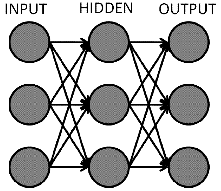
The activity of each hidden unit is determined by the activities of the input units and the weights on the connections between the inputs and the hidden units. The behavior of the output units depends on the activity of the hidden units and the weights between the hidden and output units. For this study temperature, humidity and pressure have been selected as inputs and anodic charge as output variable. It was demonstrated[13] that the number of layers is not critical for the network performance, so we decided to go with 3 layers and give to the neural network a sufficient number of hidden units automatically optimized by a genetic algorithm that can take into account several configurations.

For each configuration a genetic algorithm performs the training process with an estimation of the global error; then the configuration is stored and the genetic algorithm continues to evaluate a slightly different configuration. Once the algorithm has taken into account all the possible configurations the best one in terms of global error is chosen.

During the training phase the network is taught with environmental data as input, the output depends on the neuronal weights, that at the very beginning are initialized with random numbers. The network output is compared to the experimental data we want to model, then the network estimates the error and modifies the neurons weights in order to minimize the estimated error.

The training phase consists of determining both weights and configuration (nunber of neurons and number of layers) by minimizing the error, i.e., the difference between data and output.

3 Environmental variables and datasets

The environmental variables are monitored by an Oregon Scientific weather station WMR100. The DAQ has been modified in order to acquire via USB the environmental informations and merge environmental variables with output variables. The accuracy of the temperature sensor is $\pm 1^{o}$C in the range $0-40^{o}$C and the resolution is $0.1^{o}$C. The relative humidity sensor has an operating range from 2% to 98% with a 1% resolution, $\pm 7\%$ absolute accuracy from $25\%$ to $40\%$, and $\pm 5\%$ from $40\%$ to $80\%$. The barometer operational range is between 700 mbar and 1050 mbar with a 1 mbar resolution and a $\pm 10$ mbar accuracy.

The online monitoring system records the ambient temperature, pressure and humidity of the GGM box that contains the RPC stack. Pressure and temperature are mainly responsible of different detector behavior as well as the humidity for the bakelite and gas properties.

The used dataset is composed of four periods, each period composed of runs (about 270 each). Each run contains $10^{4}$ cosmic ray events where environmental variables and GGM anodic output charges (Q) are collected. The acquisition rate is typically 9.5 Hz.

4 Results

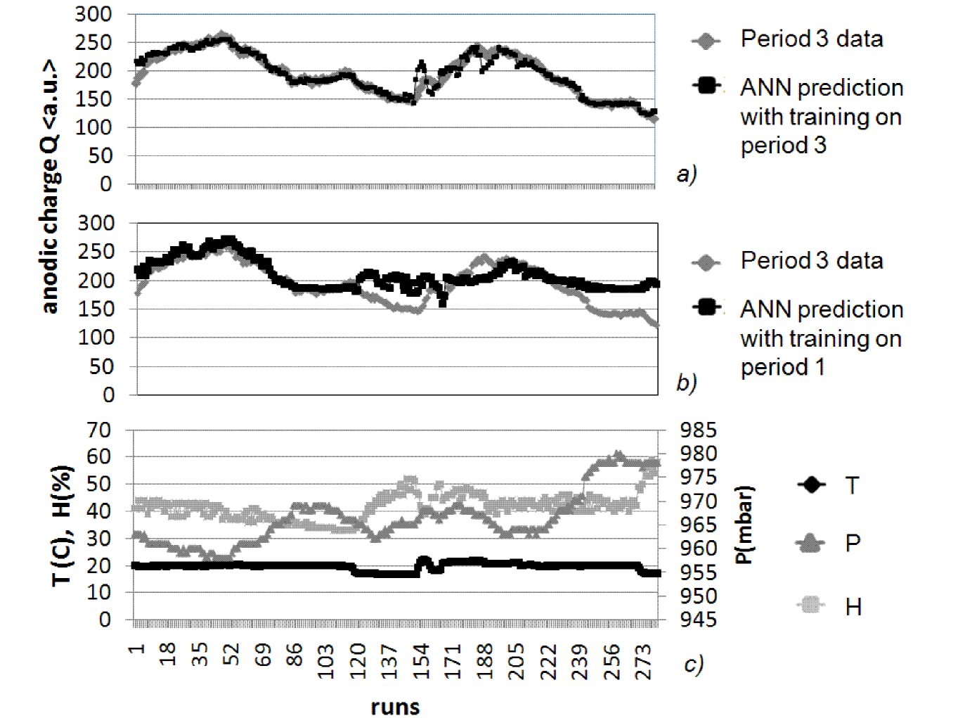
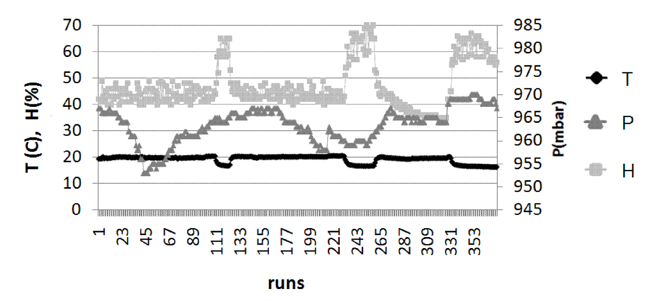
Typical ANN outputs show generally good agreement between data and prediction during training phase. (Fig. 2 $(a)$). In periods where the prediction is not accurate, the discrepancy is typically concentrated in narrow regions (“spikes”). Fig 2 $(b)$ shows the prediction on period 3 using the period 1 as training, the discrepancy around run 137 and run 256 are due to a set of environmental variables not available in the training period as shown in Fig. 2 $(c)$ and Fig. 3.

Figure 2: $(a)$ Gap 7 trained on the period 3 - prediction on period 3; the prediction is performed on the same period used as training with very good agreement between experimental data and prediction. $(b)$ Gap 7 trained on the period 1 - prediction on period 3, the prediction is performed on a period different from the training one, the agreement depends on dispersion of environmental variables. $(c)$ Environmental variables during the period 3.

Figure 3: Environmental variables during the period 1

The comparison between data and prediction is shown in Fig. 4 where the quantity

$$\frac{\Delta Q}{Q}\equiv\frac{Q_{EXP}-Q_{ANN}}{Q_{EXP}}$$ (1)

is plotted for all four periods both for training (top) and predictions (bottom), divided for training and prediction respectively. The error distribution for the predictions is much wider than for the training, as expected.

Figure 4: Error for training (top) and prediction (bottom) for all runs. Gaussian fit superimposed. The quantity $\hat{\sigma}$ is the width of the gaussian fit to the data in a reduced range which excludes the nongaussian tails.

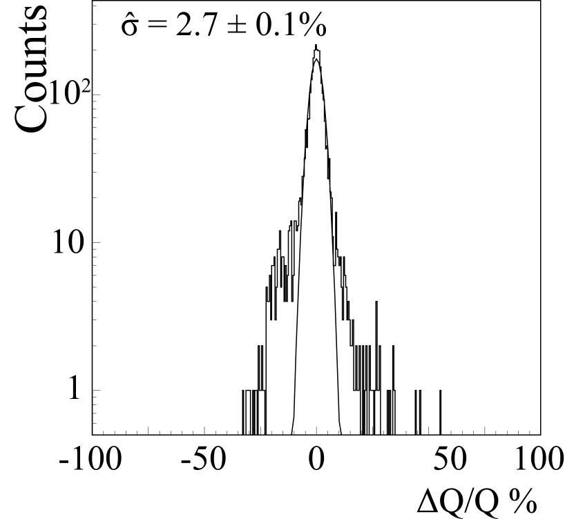
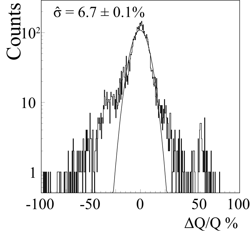
The gaussian fit superimposed (Fig. 4) is not able to fit the data properly due to the presence of large nongaussian tails, which are caused by runs with very large discrepancy between data and prediction. To evaluate the width $\hat{\sigma}$ of the error distribution we perform a gaussian fit in a reduced range which does not take into account the nongaussian tails. The distribution of the error for the predictions shows a $\hat{\sigma}$ = $6.7\%$. In the Table 3 there is a summary with error for training and predictions. The cases with very large discrepancy were studied in detail, and found to be characterized by a $(p,T,H)$ value at the edges of the variables space.

To determine the measure of the dispersion of the environmental variables considering all the runs ($N$) we computed the:

$$\frac{\Delta X}{X}\equiv\sqrt{\sum_{j=1,3}\biggr{[}\frac{(x_{j}-X_{j})}{X_{j}}\biggr{]}^{2}}$$ (2)

$$X_{j}\equiv\sum_{i=1,N}(x_{j})_{i}\quad;\quad{\bf x}\equiv(p,T,H)\quad$$ (3)

The distribution of the $\frac{\Delta Q}{Q}$ error as a function of the dispersion of environmental variables $\frac{\Delta X}{X}$ (Fig. 5) shows three distinct structures. The satellite bands with very large error were studied in detail. All data point in such bands belong to period four and gap six for which problems were detected. Period four and gap six therefore were excluded in the analysis. The distribution of the error as a function of dispersion of environmental variables after this selection has a $\hat{\sigma}\sim 4\%$ width and nongaussian tails extending up to $\frac{\Delta Q}{Q}=200\%$.

Figure 5: Distribution of $\frac{\Delta Q}{Q}$ as a function of the dispersion of environmental variables $\frac{\Delta X}{X}$ for all periods, six gaps and both training and prediction. Each training period is included once, each prediction is included 4 times, due to different training period chosen.

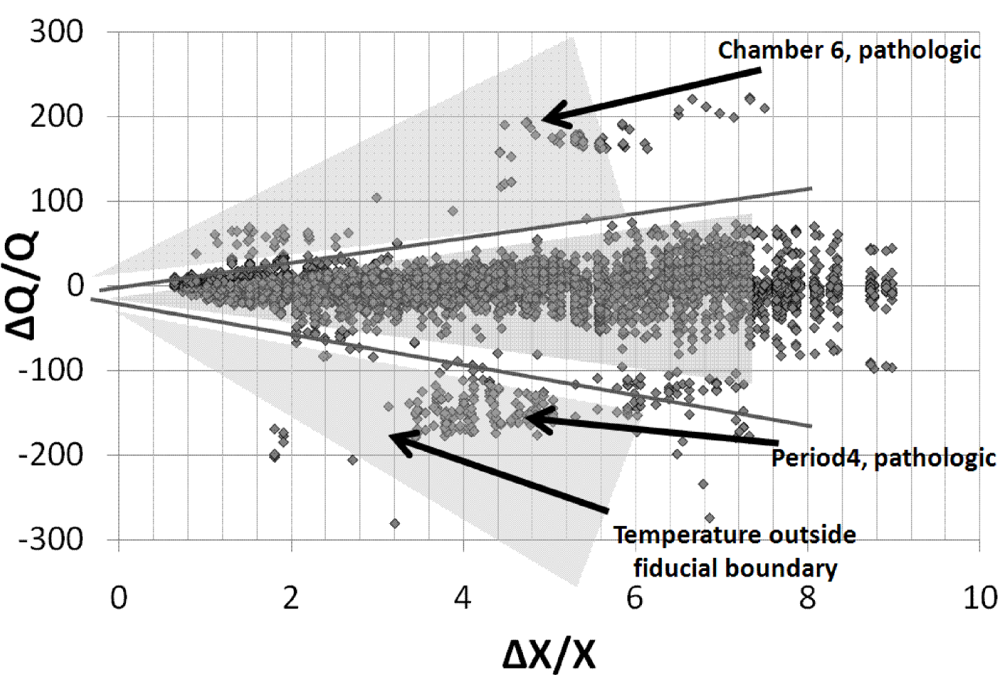
A selection on the fiducial volume in the x variables space (Table  2) was applied in order to exclude from the analysis data with $(p,T,H)$ close to the edges of the variable space. After the selection cuts, prediction on two periods based on training on the third period were performed. The nongaussian (NG) tails were defined as the fractional area outside the region $\pm 4\hat{\sigma}$. The selection cuts slightly reduce the width ($\hat{\sigma}<3.7\%$), while drastically reducing the nongaussian tails (Table 3).

Table 2: Synopsis of the selection cuts for fiducial volume applied to predicted data.

$(958<p<968){\rm mbar}$

$(19.4<T<20.4)^{o}$C

$(34<H<44)\%$

Table 3: Summary of errors $\hat{\sigma}$ and nongaussian (NG) tails for various selection cuts and samples.

Data sets	$\hat{\sigma}$	NG tail
	%	%
All six chambers, all four periods training	$2.7$	$2.26$
All six chambers, all four periods prediction	$6.7$	$6.60$
Chamber six and period four excluded prediction	$3.0$	$4.63$
Predict. on per. 2 and 3, train. on per. 1	$4.0$	$3.52$
Predict. on per. 3 and 1, train. on per. 2	$3.4$	$2.95$
Predict. on per. 1 and 2, train. on per. 3	$3.8$	$1.63$
Predict. on per. 2 and 3, train. on per. 1, fiducial cuts	$3.7$	$0.49$
Predict. on per. 3 and 1, train. on per. 2, fiducial cuts	$2.9$	$0.98$
Predict. on per. 1 and 2, train. on per. 3, fiducial cuts	$3.3$	$0.29$

5 Discussion

In this study the GGM is the system used to train the neural network with anode charge as output variable and $(p,T,H)$ as input variable. The addition of the dark current as a output variable and dose as input variable is expected to improve predictions and will be implemented. The main advantage of this approach is that several variables can be used together in order to predict chamber behavior without the needs of studying the surface corrosion, environmental/radiation dependence and bakelite aging due to chemical reactions and deposits; also in the ANN analysis, given enough data, it is possible to decouple the effect of the chosen variables used as output. This approach, once properly trained, could spot immediately and online pathological chambers whose behavior is shifting from the normal one. Further studies are in progress to determine and cure the residual nongaussian tails of the $\frac{\Delta Q}{Q}$ errors distributions, to deal with training and prediction on detectors with different high voltage supply, to widen the sample of environmental conditions, and in adding new dimensions to the variables space such as radiation levels.

6 Conclusions

A new approach for modeling the RPC behavior, based on ANN, has been introduced and preliminary results obtained using data from the CMS RPC GGM system. The ANN was trained for predicting the behavior of the anode charge Q (output variables) as function of the environmental variables $(p,T,H)$ (input variables), resulting in a prediction error $\frac{\Delta Q}{Q}=4\%$. In a forthcoming work we plan to include the dose as input variable and the dark current as output variable, aiming at a further improvement on the predictions.

Acknowledgements

The skills of M. Giardoni, L. Passamonti, D. Pierluigi, B. Ponzio and A. Russo (Frascati) in setting up the experimental setup are gratefully acknowledged. The technical support of the CERN gas group is gratefully acknowledged. Thanks are due to R. Guida (CERN Gas Group), Nadeesha M. Wickramage, Yasser Assran for discussions and help. This research was supported in part by the Italian Istituto Nazionale di Fisica Nucleare and Ministero dell’ Istruzione, Università e Ricerca.

References

- [1] R. Santonico and R. Cardarelli, Nucl. Instrum. Meth. 187 (1981) 377.
- [2] CMS Collaboration, JINST 0803 (2008) S08004. doi:10.1088/1748-0221/3/08/S08004.
- [3] The ATLAS Collaboration, G. Aad et al., CERN Large Hadron Collider , JINST 3 (2008) S08003.
- [4] G. D’Ali Staiti [ARGO-YBJ Collaboration], Nucl. Instrum. Meth. A 588 (2008) 7.
- [5] P. Fonte, IEEE Transactions on Nuclear Science, vol. 49, no. 3, June 2002.
- [6] CMS Collaboration, JINST 3 (2008) S08004.
- [7] CMS Collaboration,CERN-LHCC-97-032 ; CMS-TDR-003. Geneva, CERN, 1997.
- [8] L. Benussi et al., CMS NOTE 2010/076.
- [9] M. Abbrescia et al., LNF-06-34-P, LNF-04-25-P, Jan 2007. 9pp. Presented by S. Bianco on behalf of the CMS RPC Collaboration at the 2006 IEEE Nuclear Science Symposium (NSS), Medical Imaging Conference (MIC) and 15th International Room Temperature Semiconductor Detector Workshop, San Diego, California, 29 Oct - 4 Nov 2006. arXiv:physics/0701014.
- [10] L. Benussi et al., Nucl. Instrum. Meth. A 602 (2009) 805 [arXiv:0812.1108 [physics.ins-det]].
- [11] L. Benussi et al., JINST 4 (2009) P08006 [arXiv:0812.1710 [physics.ins-det]].
- [12] W. S. Mc Culloch, W. Pitts, Bulletin of Mathematical Biophysics 5 (1943) 115.
- [13] K. Hornik, M. Stinchcombe and H. White, Neural Networks, vol. 2, pp. 359, 1989.