Multilayer multi-configuration time-dependent Hartree method: implementation and applications to a Henon-Heiles Hamiltonian and to pyrazine.

Abstract

The multilayer multiconfiguration time-dependent Hartree (ML-MCTDH) method is discussed and a fully general implementation for any number of layers based on the recursive ML-MCTDH algorithm given by Manthe [J. Chem. Phys. 128, 164116 (2008)] is presented. The method is applied first to a generalized Henon-Heiles (HH) Hamiltonian. For 6D HH the overhead of ML-MCTDH makes the method slower than MCTDH, but for 18D HH ML-MCTDH starts to be competitive. We report as well 1458D simulations of the HH Hamiltonian using a seven layer scheme. The photoabsorption spectrum of pyrazine computed with the 24D Hamiltonian of Raab et. al. [J. Chem. Phys. 110, 936 (1999)] provides a realistic molecular test case for the method. Quick and small ML-MCTDH calculations needing a fraction of the time and resources of reference MCTDH calculations provide already spectra with all the correct features. Accepting slightly larger deviations, the calculation can be accelerated to take only 7 minutes. When pushing the method towards convergence, results of similar quality than the best available MCTDH benchmark, which is based on a wavepacket with $4.6\times 10^{7}$ time-dependent coefficients, are obtained with a much more compact wavefunction consisting of only $4.5\times 10^{5}$ coefficients and requiring a shorter computation time.

I Introduction

The multiconfiguration time-dependent Hartree (MCTDH) method mey90:73 ; man92:3199 ; bec00:1 ; mey03:251 ; mey09:book has become over the last decade the tool of choice to accurately describe the dynamics of complex multidimensional quantum mechanical systems, providing in many cases reference results that are used to benchmark other approaches or determine the behavior of approximate methods. MCTDH was initially formulated with molecular quantum dynamics in mind, where the degrees of freedom are distinguishable and the potential operator correlates in principle all vibrational degrees of freedom of the system. Many successful applications over the years deal with the spectroscopy of molecules raa99:936 ; mar05:204310 ; dor08:224109 ; wor08:569 ; ven09:034308 , isomerisation and intramolecular vibrational energy redistribution (IVR) ric04:6072 ; iun04:6992 , inelastic and reactive scattering calculations suk02:10641 ; ott08:064305 ; wu04:2227 ; har07:084303 ; bha10:214304 , scattering of atoms or molecules at surfaces hei01:1382 ; har04:3829 ; cre06:074706 , etc. More recently, the potential of the MCTDH method for the treatment of systems of indistinguishable particles, either fermions or bosons, has been realized as well, and many applications can be counted nowadays in such new directions sak09:2206011 ; alo09:301 ; zoe08:040401 ; zan04:763 ; jor08:025035 ; nes07:214106 ; suk09:223002 . Although the equations of motion remain the same in such cases, the symmetry properties of the wavefunction and the often two-body nature of the interactions has lead to the appearance of dedicated programs that specifically and efficiently deal with such cases zan03:1064 ; nes05:124102 ; alo08:033613 .

In general, the solution of the time-dependent Schrödinger equation in a direct-product basis of 1D functions (primitive functions) scales exponentially as $N^{f}$, where $N$ is the number of primitive basis functions per degree of freedom and $f$ is the number of degrees of freedom. In the MCTDH ansatz one introduces an optimal time-dependent (TD) basis (called SPF for single particle function) for each degree of freedom, which can be kept smaller than the underlying primitive basis, leading to a better scaling of the number of configurations $n^{f}$. In this way, MCTDH can deal with larger systems than the standard method, although the exponential scaling with $f$ remains, but to a lower base. The base can be further reduced by grouping degrees of freedom together in what are called combined modes or logical coordinates. One obtains in this way a smaller number of effective degrees of freedom $p$, leading to a smaller number of configurations, but the TD basis functions that have to be now propagated are multidimensional. For a given problem, it is possible to find mode-combination schemes that provide an optimum balance between the effort of propagating the expansion coefficients of each configuration (the A-vector in usual MCTDH terminology) and the effort of propagating the multidimensional SPFs . With increasing dimensionality, however, the multidimensional SPFs, the A-vector, or both, become harder and harder to propagate. As a rule of thumb and very generally, the number of degrees of freedom that can be treated for a correlated vibrational problem nowadays is about 20, but for systems well suited for MCTDH more than 60 degrees of freedom (DOF) have been accounted for wan00:9948 ; nes03:24 .

Multilayer (ML) MCTDH represents a powerful extension of the usual MCTDH approach, in which a multiconfigurational ansatz is used for the multidimensional SPFs themselves. This results in an extra layer of TD coefficients that have to be propagated and hence the name. One way to think of the ML wavefunction ansatz (given below) is to see the standard propagation method and MCTDH as particular cases of a ML wavefunction. In the standard propagation method a single layer of expansion coefficients with respect to some time-independent (TI) basis is present. MCTDH contains a first layer of expansion coefficients with respect to the SPF basis, and a second layer of TD expansion coefficients that parameterize the time evolution of the SPFs. Expanding multidimensional SPFs using a MCTDH-like ansatz one obtains a three-layer scheme. Schemes with more than three layers are of course possible. In passing we note that the ML-MCTDH ansatz can be connected to tensor contraction techniques in the mathematical literature chi07:084110 and to density matrix renormalization group (DMRG) theory whi99:4127 .

ML-MCTDH was first formulated by Wang and Thoss, who also provided an implementation of the method for three layers (in the present paper MCTDH is regarded as a two-layer scheme) and showed its applicability on the spin-boson model and on an electron-transfer model wan03:1289 . A formally identical formulation, but without an implementation, was given independently at the same time by Meyer and Worth mey03:251 , who termed it cascading MCTDH. Over the last years Wang and Thoss have further developed ML-MCTDH, expanding the number of layers that their code can handle and treating condensed phase model Hamiltonians of large dimensionality between 100 and a few thousand DOF wan06:034114 ; cra07:144503 ; kon07:11970 ; wan08:115005 . The same authors also described how ML-MCTDH can be used to deal with identical particles, which is accomplished defining the problem in Fock space and directly working in the occupation-number representation wan09:024114 . (Note that ML-MCTDH cannot be applied to identical particles in the usual first-quantized formulation because the grouping of DOF into combined modes destroys the necessary exchange symmetry properties of the wavefunction.) Recently, Manthe provided a recursive formulation of the ML-MCTDH equations of motion (EOM) for any number of layers and described the recursive algorithm that has to be used to compute all quantities entering the EOM man08:164116 ; man09:054109 .

In this contribution, we present the implementation of the EOM and recursive algorithm proposed by Manthe, and discuss its applicability and performance on a Henon-Heiles (HH) model system and on a realistic non-adiabatic molecular case, full dimensional 24D pyrazine. The resulting implementation is fully general and it can handle standard method (one layer), normal MCTDH (two layers) and any desired multilayering scheme. In this paper, we report on simulations with three layers and up to a seven-layer case for the 1458D HH Hamiltonian. We also simulate pyrazine using five and six layer schemes. The ML-MCTDH concept, EOM and recursive algorithm are discussed first, emphasizing some aspects of our implementation such as the treatment of the separable parts of the Hamiltonian. We have tried to keep such discussion self-contained and to reflect the way our code operates, but for an in-deep discussion Ref. man08:164116 should be read. The performance and correctness of the recursive implementation are tested on the HH Hamiltonian. For this system, 6D calculations with varying coupling strength are carried on first, which are directly compared to MCTDH results. For such a low dimensionality, the algorithmic complexity of ML-MCTDH does not yet pay off, and MCTDH is more efficient than ML-MCTDH. For 18D HH we find that ML-MCTDH starts to be competitive. For this case we analyze the convergence properties of the method with respect to the number of basis functions at each layer. Simulations of 1458D HH are also reported, showing the power of this approach. The ML-MCTDH implementation is then applied to the photoabsorption spectrum of pyrazine using the 24D vibronic-coupling Hamiltonian of Raab and coworkers raa99:936 . This is a realistic molecular Hamiltonian involving the presence of a conical intersection between the electronic state $S_{2}$ initially populated by photoabsorption and the $S_{1}$ electronic state to which the system decays within some ten fs. The Hamiltonian of Ref. raa99:936 has been used to test several quantum dynamical approaches. In the case of ML-MCTDH, we find that the method performs very efficiently and provides already well converged spectra in about a fifth of the CPU time used by the smallest of the MCTDH reference results using extremely few computational resources. Tolerating a larger error one can reduce the computation time to 7 minutes and still get a spectrum with all basic features in place. This is amazingly fast, considering that one is dealing with a fully correlated 24-dimensional quantum dynamics calculation. No other quantum dynamical method applied up to date to the pyrazine Hamiltonian offers the extreme quality/cost relation provided by ML-MCTDH. When pushing ML-MCTDH towards convergence with the pyrazine Hamiltonian, we find that it still offers results of at least the same quality (if not better) than the best benchmark results available from MCTDH calculations with about $4\times 10^{7}$ configurations, at a lower computational cost.

The paper is organized as follows: Section II discusses the ML-MCTDH equations and implementation. Section III.1 discusses the results on the HH Hamiltonian and Section III.2 discusses the application of ML-MCTDH to the photoabsorption spectrum of pyrazine. Section IV summarizes the results and provides some future perspectives for the method.

II Multilayer MCTDH

II.1 Ansatz and general concept

The wavefunction of a system of distinguishable degrees of freedom, e.g. representing molecular vibrations, can be conveniently represented as an expansion in terms of direct products of orthonormal basis functions, one for each degree of freedom

$$\Psi(q_{1},\ldots,q_{f},t)=\sum_{j_{1}}^{N_{1}}\cdots\sum_{j_{f}}^{N_{f}}A_{j_{1},\ldots,j_{f}}^{1}(t)\cdot\chi_{j_{1}}^{(1)}(q_{1})\cdot\ldots\cdot\chi_{j_{f}}^{(f)}(q_{f}).$$ (1)

Following the notation introduced by Manthe man08:164116 , the $A_{j_{1},\ldots,j_{f}}^{1}$ denote the TD coefficients of the first (and by now the only) layer of TD expansion terms.

In the MCTDH approach, the wavefunction is expanded in terms of direct products of orthonormal time-dependent single particle functions (SPF)

$$\Psi(q_{1},\ldots,q_{f},t)=\sum_{j_{1}}^{n_{1}}\cdots\sum_{j_{f}}^{n_{f}}A_{j_{1},\ldots,j_{f}}^{1}(t)\cdot\varphi_{j_{1}}^{(1;1)}(q_{1},t)\cdot\ldots\cdot\varphi_{j_{f}}^{(1;f)}(q_{f},t),$$ (2)

which are themselves expanded in terms of the underlying primitive basis

$$\varphi_{m}^{1;\kappa}(q_{\kappa},t)=\sum_{j}^{N_{\kappa}}A_{m;j}^{2;\kappa}(t)\cdot\chi_{j}^{(\kappa)}(q_{\kappa}).$$ (3)

Therefore, MCTDH can be seen as a 2-layer scheme with TD coefficients $A_{j_{1},\ldots,j_{f}}^{1}(t)$ at the top layer, and sets of second layer TD coefficients $A_{m;j}^{2;\kappa}(t)$ for each degree of freedom. We usually refer to the 1-layer scheme as the standard method, to the 2-layer scheme simply as MCTDH, and to deeper layering schemes as ML-MCTDH. Note the important detail that all SPFs of a certain degree of freedom are expanded in terms of the same underlying basis, i.e. the $\chi_{j}^{(\kappa)}(q_{\kappa})$ functions in Eq. (3) have no $m$ index.

The computational gain of MCTDH with respect to the standard method arises from the expansion orders $n_{\kappa}$ being in general smaller than the size of the underlying primitive basis $N_{\kappa}$, which leads to a smaller number of TD coefficients to be propagated. However, the total number of TD coefficients is still given by $\prod_{\kappa=1}^{f}n_{\kappa}$, and therefore the computational effort raises exponentially with the number of degrees of freedom. Hence, MCTDH does not eliminate the exponential scaling but reduces the base to which the scaling occurs (for a detailed analysis of the computational scaling of MCTDH see for example Ref. bec00:1 ). The base can be further reduced by combining the physical coordinates $q_{1},\ldots,q_{f}$ into logical coordinates (also referred to as combined modes) $Q_{1}^{1},\ldots,Q_{p}^{1}$, such that each logical coordinate comprises one or several of the physical coordinates, as $Q_{\kappa}^{1}=\{q_{1_{\kappa}},\ldots,q_{d_{\kappa}}\}$. Here a more general notation to designate a combined coordinate has been introduced, that will be useful when discussing deeper layering schemes. Mode combination has been extensively used in many applications of the MCTDH method. Similarly as in Eq. (2), the MCTDH wavefunction now reads

$$\Psi(Q_{1}^{1},\ldots,Q_{p}^{1},t)=\sum_{j_{1}}^{n_{1}}\cdots\sum_{j_{p}}^{n_{p}}A_{1;j_{1},\ldots,j_{p}}^{1}(t)\cdot\varphi_{j_{1}}^{(1;1)}(Q_{1}^{1},t)\cdot\ldots\cdot\varphi_{j_{p}}^{(1;p)}(Q_{p}^{1},t),$$ (4)

and the TD basis functions $\varphi_{j_{\kappa}}^{(1;\kappa)}(Q_{\kappa}^{1},t)$ are now multidimensional. Introducing mode-combination, the computational effort is switched from the propagation of a large vector of $A_{j_{1},\ldots,j_{p}}^{1}(t)$ coefficients and one-dimensional SPFs, to a shorter vector of coefficients but multi-dimensional, harder to propagate SPFs. It is often the case, that some experience and knowledge of the system under consideration is necessary to find an efficient mode-combination scheme for a given problem. The mode-combined SPFs are given by

$$\varphi_{m}^{1;\kappa}(Q_{\kappa}^{1},t)=\sum_{j_{1_{\kappa}}}^{N_{1_{\kappa}}}\cdots\sum_{j_{d_{\kappa}}}^{N_{d_{\kappa}}}A_{m;j_{1_{\kappa}},\ldots,j_{d_{\kappa}}}^{2;\kappa}(t)\cdot\chi_{j_{1_{\kappa}}}^{(\kappa,1)}(Q_{1_{\kappa}}^{2;\kappa})\cdot\ldots\cdot\chi_{j_{d_{\kappa}}}^{(\kappa,d_{\kappa})}(Q_{d_{\kappa}}^{2;\kappa}),$$ (5)

where the last equation resembles the ansatz in Eq. (1) in that multidimensional SPFs are represented as a multiconfigurational expansion in terms of underlying time-independent basis functions. In the same way a TD basis was introduced above in going from the standard ansatz to MCTDH, effectively adding a second layer of TD expansion coefficients, an MCTDH expansion can be used to represent the $\varphi_{m}^{1;\kappa}(Q_{\kappa}^{1},t)$ SPFs, effectively adding a third layer of expansion coefficients. This results in a 3-layer ML-MCTDH ansatz.

The ML-MCTDH layering scheme can be very flexible. In a high dimensional system one combines groups of degrees of freedom into high dimensional SPFs until the size of the vector of coefficients in Eq. (4) becomes manageable. However, the combined SPFs are too large to be efficiently propagated. Then, one breaks the combined modes into even smaller groups of logical coordinates introducing a new layer of coefficients, whose size is manageable. This procedure can be repeated over and over until the (possibly combined) primitive degrees of freedom are reached.

Owing to the flexibility of the layering scheme, and the fact that ML-MCTDH wavefunctions can be many layers deep, it is convenient to introduce a diagrammatic notation to represent these objects man08:164116 . In this notation, wavefunctions are represented by trees, i.e. connected graphs without loops. Each node in the tree represents a set of vectors of coefficients $A_{m;j_{1},\ldots,j_{p_{\kappa_{l}}}}^{l;\kappa_{1},\ldots,\kappa_{l-1}}$, where $l$ denotes the layer depth, $\kappa_{1},\ldots,\kappa_{l-1}$ denote the indices of the logical degrees of freedom starting from the top node and down to a particular node (path from the top down to a given node), $m$ indicates the different vectors within this node, and finally $j_{1},\ldots,j_{p_{\kappa_{l}}}$ are the tensor indices of each particular array of coefficients within the node.

Some ML diagrams are presented later when discussing the various applications (see Figs. 1,4,9). The lines connecting one node with its descendant nodes in such diagrams represent the tensor indices $j_{1},\ldots,j_{p_{\kappa_{1},\ldots,\kappa_{l}}}$, one line per index, and the numbers at the side of each line refer to the maximum possible value of the corresponding index. Each node is uniquely described by the values of its label $({l;\kappa_{1},\ldots,\kappa_{l-1}})$.

II.2 ML-MCTDH equations of motion and recursive implementation

The ML-MCTDH equations of motion (EOM) have been derived and discussed by Wang and Thoss wan03:1289 and Manthe man08:164116 . In Ref. man08:164116 a fully general derivation of the ML-MCTDH EOM for arbitrary layering schemes is provided, together with an algorithm for the recursive evaluation of all intermediate quantities entering the EOM. We reproduce here the EOM and hint the key elements of the recursive algorithm for the sake of completeness. Later we discuss some specific aspects of our implementation.

The ML-MCTDH EOM have a very similar structure to the usual MCTDH equations, and for the top layer coefficients they are identical to the MCTDH ones

$$i\frac{\partial A_{I}^{1}}{\partial t}=\sum_{J}\langle\Phi_{I}^{1}|\hat{H}|\Phi_{J}^{1}\rangle A_{J}^{1},$$ (6)

where the top layer configurations $\Phi_{J}^{1}=\varphi_{j_{1}}^{(1;1)}(Q_{1}^{1},t)\cdot\ldots\cdot\varphi_{j_{p}}^{(1;p)}(Q_{p}^{1},t)$, are defined as direct products of SPFs and the multi-index $J=j_{1},\ldots,j_{p}$ has been implicitly introduced. The EOM for the propagation of the SPFs are formally the same for all layers

$$i\frac{\partial\varphi_{n}^{z,\kappa_{l}}}{\partial t}=(1-\hat{P}_{\kappa_{l}}^{z})\sum_{j,m}(\rho^{z,\kappa_{l}})_{nj}^{-1}\cdot\langle\hat{H}\rangle_{jm}^{z,\kappa_{l}}\varphi_{m}^{z,\kappa_{l}},$$ (7)

where $\hat{P}_{\kappa_{l}}^{z}=\sum_{j}|\varphi_{j}^{z,\kappa_{l}}\rangle\langle\varphi_{j}^{z,\kappa_{l}}|$ is the projector onto the space spanned by the $\varphi_{j}^{z,\kappa_{l}}$ SPFs, $\rho^{z,\kappa_{l}}$ is a density matrix and $\langle\hat{H}\rangle^{z,\kappa_{l}}$ is a matrix of mean-field operators acting on the $\varphi_{j}^{z,\kappa_{l}}$ functions. The symbol $z$ is a shorthand for the indices specifying a node, $z={l;\kappa_{1},\ldots,\kappa_{l-1}}$, and for further reference we introduce $z\!-\!1={l-1;\kappa_{1},\ldots,\kappa_{l-2}}$, and similar for $z\!+\!1$. In its form above, the EOM for the SPFs look identical to the usual EOM for the SPFs in the usual MCTDH bec00:1 . Only the computation of the density matrices and mean-fields entering the EOM is now more involved than in a single-layer MCTDH scheme.

Before describing how in practice the recursive calculation of mean-fields and density matrices is performed, we first restrict ourselves to the case in which the Hamiltonian is given by sums of products of operators acting on the primitive (but possibly combined) degrees of freedom $Q_{\kappa}^{\text{prim}}$

$$\hat{H}=\sum_{r=1}^{s}c_{r}\hat{H}_{r}=\sum_{r=1}^{s}c_{r}\prod_{\kappa=1}^{f}\hat{h}_{r}^{(\mathrm{prim};\kappa)}.$$ (8)

This form of the operator is necessary to avoid the computation of high dimensional integrals, and has been thoughtfully discussed in the MCTDH literature. Terms which usually do not follow the product form are, e.g. general potential energy surfaces. There exist however algorithms to bring general potentials to product form jae96:7974 ; jae98:3772 ; lat00:1253 ; lat00:1324 . Furthermore, MCTDH and ML-MCTDH formulations based on time-dependent grids that by-pass this restriction (so-called CDVR approach) have also been provided man96:6989 ; man08:164116 , but here we always will assume Hamiltonians in product form, Eq. (8).

In order to discuss the practical computation of the mean-field elements $\langle\hat{H}\rangle_{jm}^{l;\kappa_{1},\ldots,\kappa_{l}}$ appearing in Eq. (7), we center our attention on a particular node $z=({l;\kappa_{1},\ldots,\kappa_{l-1}})$. This node relates to the logical coordinate $Q_{\kappa_{l-1}}^{l-1;\kappa_{1},\ldots,\kappa_{l-2}}$, which can be further decomposed into a combination of logical coordinates

$$Q_{\kappa_{l-1}}^{z\!-\!1}=\{Q_{1}^{z},\ldots,Q_{p_{\kappa_{l}}}^{z}\},$$ (9)

and holds vectors of coefficients denoted by $A_{m;j_{1},\ldots,j_{p_{\kappa_{l}}}}^{z}$. These coefficients are expansion coefficients of SPFs in layer $l\!-\!1$ expanded in terms of SPFs in layer $l$. This is better seen by extending Eqs. (3,5) to the fully general multilayer case

$$\varphi_{m}^{{z\!-\!1,\kappa_{l-1}}}(Q_{\kappa_{l-1}}^{z\!-\!1}) = \sum_{j_{1}}^{n_{1}}\cdots\sum_{j_{p_{\kappa_{l}}}}^{n_{\kappa_{l}}}A_{m;j_{1},\ldots,j_{p_{\kappa_{l}}}}^{z}\prod_{\kappa_{l}=1}^{p_{\kappa_{l}}}\varphi_{j_{\kappa_{l}}}^{z,\kappa_{l}}(Q_{\kappa_{l}}^{z})$$ (10a)

$$= \sum_{J}A_{m;J}^{z}\cdot\Phi_{J}^{z}(Q_{\kappa_{l-1}}^{z\!-\!1}),$$ (10b)

where the configurations $\Phi_{J}^{z}$ are the multilayer generalization of the configurations introduced in Eq. (6). The operator summands in Eq. (8) can be written as

$$\hat{H}_{r} = \hat{\mathcal{H}}_{r}^{l;\kappa_{1},\ldots,\kappa_{l}}\cdot\hat{h}_{r}^{l;\kappa_{1},\ldots,\kappa_{l}}$$ (11a)

$$= \hat{\mathcal{H}}_{r}^{l;\kappa_{1},\ldots,\kappa_{l}}\cdot\prod_{\kappa_{l+1}=1}^{p_{\kappa_{l+1}}}\hat{h}_{r}^{{l+1;\kappa_{1},\ldots,\kappa_{l+1}}},$$ (11b)

where $\hat{h}_{r}^{l;\kappa_{1},\ldots,\kappa_{l}}$ acts on the logical coordinate $Q_{\kappa_{l}}^{l;\kappa_{1},\ldots,\kappa_{l-1}}$, while $\hat{\mathcal{H}}_{r}^{l;\kappa_{1},\ldots,\kappa_{l}}$ acts on the corresponding remaining space. As seen from Eq. (11b), $\hat{h}_{r}^{l;\kappa_{1},\ldots,\kappa_{l}}$ can as well be written as a direct product of operators $\hat{h}_{r}^{{l+1;\kappa_{1},\ldots,\kappa_{l+1}}}$, which act on logical coordinates $Q_{\kappa_{l+1}}^{l+1;\kappa_{1},\ldots,\kappa_{l}}$. In fact, both operators $\hat{\mathcal{H}}_{r}^{l;\kappa_{1},\ldots,\kappa_{l}}$ and $\hat{h}_{r}^{l;\kappa_{1},\ldots,\kappa_{l}}$ can be broken down to a simple product of operators which act on one primitive (but possibly combined) coordinate only (see Eq. (8)). The matrix elements of the mean-field operators at the right-hand-side of Eq. 7 for one particular summand $\hat{H}_{r}$ are given by

$$\langle\hat{H}_{r}\rangle_{jm,IJ}^{{z,\kappa_{l}}}=\langle\Phi_{I}^{z\!+\!1}|\langle\hat{H}_{r}\rangle_{jm}^{{z,\kappa_{l}}}|\Phi_{J}^{z\!+\!1}\rangle,$$ (12)

which is readily seen if the SPFs in Eq. (7) are written in their explicit form given in Eq. (10b). These are the most cumbersome quantities to compute within the ML-MCTDH scheme. By substituting Eqs. (11a,b) into Eq. (12) one arrives at

$$\langle\hat{H}_{r}\rangle_{jm,IJ}^{l;\kappa_{1},\ldots,\kappa_{l}} = \langle\hat{\mathcal{H}}_{r}^{l;\kappa_{1},\ldots,\kappa_{l}}\rangle_{jm}^{l;\kappa_{1},\ldots,\kappa_{l}}\cdot\left[\hat{h}_{r}^{l;\kappa_{1},\ldots,\kappa_{l}}\right]_{IJ}$$ (13a)

$$= \langle\hat{\mathcal{H}}_{r}^{l;\kappa_{1},\ldots,\kappa_{l}}\rangle_{jm}^{l;\kappa_{1},\ldots,\kappa_{l}}\cdot\prod_{\kappa_{l+1}=1}^{p_{\kappa_{l+1}}}\left[\hat{h}_{r}^{{l+1;\kappa_{1},\ldots,\kappa_{l+1}}}\right]_{i_{\kappa_{l+1},j_{\kappa_{l+1}}}}$$ (13b)

with

$$\left[\hat{h}_{r}^{z,\kappa_{l}}\right]_{IJ} = \langle\Phi_{I}^{z\!+\!1}|\hat{h}_{r}^{{z,\kappa_{l}}}|\Phi_{J}^{z\!+\!1}\rangle$$ (14a)

$$\left[\hat{h}_{r}^{{z\!+\!1,\kappa_{l+1}}}\right]_{i_{\kappa_{l+1},j_{\kappa_{l+1}}}} = \langle\varphi_{i_{\kappa_{l+1}}}^{{z\!+\!1,\kappa_{l+1}}}|\hat{h}_{r}^{{z\!+\!1,\kappa_{l+1}}}|\varphi_{j_{\kappa_{l+1}}}^{{z\!+\!1,\kappa_{l+1}}}\rangle$$ (14b)

(The mean-field tensor $\langle\hat{\mathcal{H}}_{r}^{z,\kappa_{l}}\rangle_{jm}^{z,\kappa_{l}}$ will be discussed below, Eq. (II.2)). It remains therefore to be seen, how the quantities appearing in the right-hand-side of Eq. (13b) can be recursively computed.

The expression for the $h$-matrices is found by starting from Eq. (14b) and explicitly writing the SPFs in layer $l+1$ in terms of those in layer $l+2$

$$\left[\hat{h}_{r}^{{z\!+\!1,\kappa_{l+1}}}\right]_{a_{\kappa_{l+1}},b_{\kappa_{l+1}}} = \langle\varphi_{a_{\kappa_{l+1}}}^{{z\!+\!1,\kappa_{l+1}}}|\hat{h}_{r}^{z\!+\!1,\kappa_{l+1}}|\varphi_{b_{\kappa_{l+1}}}^{{z\!+\!1,\kappa_{l+1}}}\rangle$$

$$= \langle\varphi_{a_{\kappa_{l+1}}}^{{z\!+\!1,\kappa_{l+1}}}|\displaystyle\prod_{\kappa_{l+2}=1}^{p_{\kappa_{l+2}}}\hat{h}_{r}^{{z\!+\!2,\kappa_{l+2}}}|\varphi_{b_{\kappa_{l+1}}}^{{z\!+\!1,\kappa_{l+1}}}\rangle$$

$$= \displaystyle\prod_{\kappa_{l+2}=1}^{p_{\kappa_{l+2}}}\displaystyle\sum_{J^{\kappa_{l+2}}}\displaystyle\sum_{i,j}A_{a_{k_{l+1}};J_{i}^{\kappa_{l+2}}}^{*\;z\!+\!2}\left[\hat{h}_{r}^{{z\!+\!2,\kappa_{l+2}}}\right]_{i,j}A_{b_{k_{l+1}};J_{j}^{\kappa_{l+2}}}^{z\!+\!2}.$$

Here multi-indices $J^{\kappa}$ and $J_{m}^{\kappa}$ have been introduced to make the notation more compact. The former contains all indices except for the $\kappa$-th one, while the latter has index $\kappa$ set to $m$. Eq. (II.2) tells us that the computation of the matrix elements of $\hat{h}_{r}^{{z\!+\!1,\kappa_{l+1}}}$ requires the previous knowledge of the matrix elements of $\hat{h}_{r}^{{z\!+\!2,\kappa_{l+2}}}$. Therefore, one starts at the lowest layer with the matrix elements of $\hat{H}$ with respect to the underlying time-independent basis

$$\left[\hat{h}_{r}^{l_{\mathrm{max}};\kappa_{1},\ldots,\kappa_{l_{\mathrm{max}}}}\right]_{i_{\kappa},j_{\kappa}}=\left[\hat{h}_{r}^{\mathrm{prim};\kappa}\right]_{i_{\kappa},j_{\kappa}}=\langle\chi_{i_{\kappa}}^{(\kappa)}|\hat{h}_{r}^{\mathrm{prim};\kappa}|\chi_{j_{\kappa}}^{(\kappa)}\rangle$$ (16)

where $l_{\mathrm{max}}$ denotes the maximal layer, i.e. $l_{\mathrm{max}}=2$ for normal MCTDH, and proceeds bottom up through the tree structure building the matrix representations of the $\hat{h}_{r}^{l+1;\kappa_{1},\ldots,\kappa_{l+1}}$ operators, which will subsequently be used to build the matrix elements of $\hat{h}_{r}^{l;\kappa_{1},\ldots,\kappa_{l}}$ operators, and so on.

The mean-field matrix elements are computed in practice in a similar way to Eq. (II.2). For the top layer, the mean-field elements are given as

$$\langle\hat{\mathcal{H}}_{r}^{1;\kappa_{1}}\rangle_{m,n}^{1;\kappa_{1}}=\displaystyle\prod_{\nu\neq\kappa_{1}}^{p}\displaystyle\sum_{J^{\kappa_{1},\nu}}\displaystyle\sum_{i,j}A_{1;J_{m,i}^{\kappa_{1},\nu}}^{*\;1}\left[\hat{h}_{r}^{0;\nu}\right]_{i,j}A_{1;J_{n,j}^{\kappa_{1,\nu}}}^{1},$$ (17)

where the composite indices $J^{\kappa,\nu}$ and $J_{m,n}^{\kappa,\nu}$ are defined similarly as $J^{\kappa}$ and $J_{m}^{\kappa}$. Eq. (17) corresponds to the normal way of calculating the mean-fields in standard MCTDH, and is an alternate way of writing, e.g. Eq. (67) in Ref. bec00:1 . For a given deeper layer, the calculation involves the mean-fields of the above layer and is given by man08:164116

$$\langle\hat{\mathcal{H}}_{r}^{{z,\kappa_{l}}}\rangle_{m,n}^{{z,\kappa_{l}}}=\displaystyle\sum_{a,b}\langle\hat{\mathcal{H}}_{r}^{{z\!-\!1,\kappa_{l-1}}}\rangle_{a,b}^{{z\!-\!1,\kappa_{l-1}}}$$

$$\times\displaystyle\prod_{\nu\neq\kappa_{l}}^{p_{\kappa_{l}}}\displaystyle\sum_{J^{\kappa_{l},\nu}}\displaystyle\sum_{i,j}A_{a;J_{m,i}^{\kappa_{1},\nu}}^{*\;z}\left[\hat{h}_{r}^{z\!-\!1,\nu}\right]_{i,j}A_{b;J_{n,j}^{\kappa_{1},\nu}}^{z}\;,$$ (18)

where $a$ and $b$ run over the $(l-1)$th layer SPFs, which are contained in the $l$th layer SPF $m$ and $n$, respectively. Therefore, the mean-fields can be computed if the mean-fields of the layers above, as well as the matrix elements of the $\hat{h}$ operators, are known. The density matrices are computed in a very similar way to Eq. (II.2), but application of the $\hat{h}$ matrices to $A$ vectors on the right side of Eq. (II.2) disappears. Eqs. (17-II.2) are obtained after introducing the so called single-hole functions, which are defined as the variation of the total wavefunction with respect to a particular SPF. We leave this more specialized step out of this discussion and refer the interested reader, e.g. to Refs. bec00:1 or man08:164116 .

The recursive algorithm proceeds then as follows: 1) Starting from the bottom of the tree and proceeding up, the $h$-matrix elements are evaluated after Eq. (II.2). 2) Starting from the top of the tree and proceeding down the mean-fields and density matrices are computed as in Eq. II.2. 3) The right-hand-side of the EOMs, Eqs. (6,7), is evaluated.

II.3 Separable part of the Hamiltonian across layers

The efficiency of the ML-MCTDH calculations is increased if one takes advantage of the terms $\hat{h}_{r}^{(\mathrm{prim};\kappa)}$ in Eq. (8) that are unit operators. The kinetic energy part of the Hamiltonian contains usually many unit terms. Also common models such as Henon-Heiles, vibronic Coupling, system-bath, etc. have as well many unit terms in the potential energy part of the operator.

The obvious way to obtain computational savings is to flag all unit terms as such, so that they do not have to be stored as unit matrices and they do not have to be explicitly multiplied. This is done from the bottom of the tree and proceeding recursively upwards. If all $\hat{h}_{r}^{{z\!+\!1,\kappa_{l+1}}}\equiv\hat{1}$, then $\hat{h}_{r}^{{z,\kappa_{l}}}$ is flagged as $\hat{1}$. Our implementation keeps track of all unit $h$-terms at all layers, which saves resources in the recursive construction of the $h$-matrices in Eq. (II.2), in the mean-fields construction in Eq. (II.2) and in the equations of motion.

Once the unit operators at all layers have been flagged as such, it is possible to identify non-correlated terms for a particular node, i.e. terms that decompose as

$$\hat{H}_{r}=\mathbf{1}^{{z,\kappa_{l}}}\cdot\hat{h}_{r}^{{z,\kappa_{l}}},$$ (19)

such that the non-unit parts of $H_{r}$ operate only on the combined coordinate $Q_{\kappa_{l}}^{z}$. The step of identifying separable terms is conveniently done from the top of the tree and proceeding downwards. To illustrate this let us refer to a simple 4D example and the operator summand

$$\hat{H}_{r}=\hat{h}_{r}^{\mathrm{prim};1}\cdot\hat{1}_{r}^{\mathrm{prim};2}\cdot\hat{h}_{r}^{\mathrm{prim};3}\cdot\hat{h}_{r}^{\mathrm{prim};4}.$$ (20)

The considered tree structure has four primitive nodes $(3;1,1)$, $(3;1,2)$, $(3;2,1)$ and $(3;2,2)$ with $h$-terms $\hat{h}_{r}^{3;1,1}$, $\hat{1}_{r}^{3;1,2}$, $\hat{h}_{r}^{3;2,1}$ and $\hat{h}_{r}^{3;2,2}$, which are the matrix representation of the primitive product terms in Eq. (20). The two nodes at the intermediate layer, namely $(2;1)$ and $(2;2)$, have therefore $h$-terms $\hat{h}_{r}^{2;1,1}$ and $\hat{1}_{r}^{2;1,2}$ for node $(2;1)$ and $h$-terms $\hat{h}_{r}^{2;2,1}$ and $\hat{h}_{r}^{2;2,2}$ for node $(2;2)$. The top node $(1;)$ has $h$-terms $\hat{h}_{r}^{1;1}$ and $\hat{h}_{r}^{1;2}$. Only in the case that both $\hat{h}_{r}^{2;1,1}$ and $\hat{1}_{r}^{2;1,2}$ would have been unit operators, would $\hat{h}_{r}^{1;1}$ have been marked as a unit operator as well. Now we turn to the identification of non-correlated terms starting from the top of the tree. $\hat{H}_{r}$ is marked as correlated in node $(1;)$ because both $\hat{h}_{r}^{1;1}$ and $\hat{h}_{r}^{1;2}$ are different from the unit operator. At first sight, the $\hat{H}_{r}$ term could be flagged as non-correlated in node $(2;1)$ because only one of the $h$-terms is different from unity. However, the parent node had this term marked as correlated, and therefore $\hat{H}_{r}$ is marked as correlated in node $(2;1)$. The reason why this happens is that $\hat{H}_{r}$ acts also on node $(2;2)$, which is in another branch of the tree. It is then clear that a convenient way to spot situations of this kind is to proceed recursively from the top of the tree, as illustrated. Ultimately, the $\hat{H}_{r}$ term is marked correlated in node $(2;1)$ because the mean-field matrix elements $\langle\hat{\mathcal{H}}_{r}^{2;1,1}\rangle_{m,n}^{2;1,1}$ and $\langle\hat{\mathcal{H}}_{r}^{2;1,2}\rangle_{m,n}^{2;1,2}$ correlate the motion of SPFs $\varphi_{j}^{2;1,1}$ and $\varphi_{j}^{2;1,2}$ with the dynamics proceeding in node $(2;2)$ and below. The coupling to the dynamics in the other branch arises from the relation of the mean-field elements just mentioned to the mean-fields $\langle\hat{\mathcal{H}}_{r}^{1;1}\rangle_{m,n}^{1;1}$ in the top node, as shown in Eq. (II.2).

Once the non-correlated terms have been identified for each node, one can exploit, in the same way as in standard MCTDH, that for them the mean-field matrix elements become identical to the elements of the density matrix

$$\langle\hat{\mathbf{1}}^{l;\kappa_{1},\ldots,\kappa_{l}}\rangle_{mn}^{{l;\kappa_{1},\ldots,\kappa_{l}}}\equiv(\rho^{l;\kappa_{1},\ldots,\kappa_{l}})_{mn}.$$ (21)

Hence, for a particular node with $\hat{H}_{r}$ terms $1$ to $s$ non-correlated, and terms $s+1$ to $t$ correlated, Eq. (7) can be rewritten as

$$i\frac{\partial\varphi_{n}^{z,\kappa_{l}}}{\partial t}=\left(1-\hat{P}_{\kappa_{l}}^{z}\right)\left(\sum_{q=1}^{s}c_{q}\cdot\hat{h}_{q}^{z,\kappa_{l}}+\sum_{j,m}(\rho^{z,\kappa_{l}})_{nj}^{-1}\cdot\sum_{r=s+1}^{t}c_{r}\cdot\langle\hat{\mathcal{H}}_{r}^{z,\kappa_{l}}\rangle_{jm}^{z,\kappa_{l}}\cdot\hat{h}_{r}^{z,\kappa_{l}}\right)\varphi_{m}^{z,\kappa_{l}},$$ (22)

which is the EOM for the SPFs on which our implementation is based. The EOM for the coefficients follows directly from this equation and Eq. (10)

$$\frac{\partial A_{m;J}^{z}}{\partial t}=\langle\Phi_{J}^{z}|\frac{\partial\varphi_{n}^{{z\!-\!1,\kappa_{l-1}}}}{\partial t}\rangle\;.$$ (23)

There is no contribution from $\partial{\Phi_{J}^{z}}/\partial t$ because, due to the projector, the SPFs are orthogonal to their time derivatives. Hence one may write compactly

$$\frac{\partial A_{n;J}^{z}}{\partial t}=\sum_{K}\big{(}\delta_{JK}-\sum_{j}A_{j;J}^{z}A_{j;K}^{*z}\big{)}\,\sum_{m,L}M^{z}_{n,m;KL}\,A_{m;L}^{z}\;,$$ (24)

where a detailed expression for the matrix $M^{z}_{nm;JL}$ follows from Eqs. (22, 23, 10).

As a final comment, it is worth mentioning that in large systems with groups of coordinates strongly correlated among them but weakly correlated to other groups, i.e. with some sort of locality, the identification of the correlated terms node by node may become very important. In such cases there will be many correlated terms in nodes at lower layers, but less of them as one proceeds up to the top of the tree. Such an example is given by be the HH model to be introduced below, where each harmonic oscillator is coupled only to its next neighbors. For similar reasons, when dealing with system-bath Hamiltonians with ML-MCTDH, it may be advantageous in most cases to separate system and bath already at the top layer.

III Results and Discussion

The ML-MCTDH algorithm and implementation described above are applied to two paradigmatic systems. On the one hand we simulate the HH model for various dimensionalities, and on the other hand we test our implementation on the pyrazine system using the second-order vibronic-coupling Hamiltonian of Ref. raa99:936 .

III.1 Henon-Heiles

The HH Hamiltonian

$$\hat{H}=\frac{\omega}{2}\sum_{\kappa=1}^{f}\left(-\frac{\partial^{2}}{\partial q_{\kappa}^{2}}+q_{\kappa}^{2}\right)+\lambda\sum_{\kappa=1}^{f-1}\left(q_{\kappa}^{2}\;q_{\kappa+1}-\frac{1}{3}q_{\kappa+1}^{3},\right)$$ (25)

written here in dimensionless units, offers a convenient playground to investigate the convergence properties and performance of ML-MCTDH. The HH model was used in Ref. nes02:10499 to benchmark the MCTDH method and the same Hamiltonian with similar parameters is used here for the bechmarking of ML-MCTDH. For all simulations we set $\omega=1$. The degree of anharmonicity and coupling are controlled by the single parameter $\lambda$, for which different values are chosen. The initial amount of energy in the system is easily controlled by the position at which the initial wavepacket is centered for each degree of freedom. The initial wavepacket is always taken as a Hartree product of Gaussian functions of width corresponding to the ground vibrational state of the harmonic part of the Hamiltonian. Initially, all momenta are set to zero, $\langle p_{\kappa}\rangle=0$, and similarly all positions, except for a few coordinates which are displaced by two length units with respect to $q_{\kappa}=0$. The HH Hamiltonian in Eq. (25) has dissociative channels due to the cubic terms, which are accessible in the energy range of the reported simulations. To avoid reflections from the grid edges, the Hamiltonian is augmented with a complex absorbing potential (CAP) as $H=T+V-iW$. Further details on the CAP used are found in Ref. nes02:10499 . A sine-DVR (for discrete variable representation) primitive basis with points between $-9$ and $7$ length units and $N=24$ grid points is used for all coordinates throughout the HH simulations. All propagations on HH models are carried on up to 30 time units, which roughly corresponds to five oscillation periods $T=2\pi/\omega$ in the harmonic limit.

III.1.1 6D simulations

FIGURE 1 AROUND HERE

We first concentrate on a 6D HH model. Calculations with $\lambda=\lambda_{0}$ and $\lambda=2\lambda_{0}$ are performed, for $\lambda_{0}=0.111803$. A value of $\lambda_{0}=0.111803$ allows to compare with other works that use the same Hamiltonian nes02:10499 . For the reported 6D calculations, the initial wavepacket is centered at $q_{\kappa}=2$ for coordinates $q_{2}$, $q_{4}$ and $q_{6}$. Standard MCTDH (2-layer) and ML-MCTDH calculations using a 3-layer scheme are compared, and the trees representing the MCTDH and ML-MCTDH wavefunctions are displayed in Figs. 1a and 1b, respectively. In the MCTDH case every two primitive DOF are combined, and $N_{2}$ equals the number of DVR grid points (primitive basis functions) for each DOF. In the ML-MCTDH wavefunction an extra layer of TD coefficients is introduced, effectively representing the 2D SPFs of the combined modes in the original MCTDH wavefunction by a new multiconfigurational expansion. It is worth noting that in the case of having $N_{2}=N_{3}$ for the ML-MCTDH wavefunction, the lowest layer is treated exactly and both MCTDH with mode combination and ML-MCTDH provide numerically identical results (for the same number of SPFs $N_{1}$ at the top layer).

The different propagations are compared by inspecting the autocorrelation function obtained as $a(t)=\langle\Psi^{*}(t/2)|\Psi(t/2)\rangle$. (This trick bec00:1 yields an autocorrelation function which is twice as long as the propagation). The autocorrelation at long times is difficult to converge, since the (ML-)MCTDH wavefunction accumulates error as time increases, providing an adequate quantity to compare the different propagations. Conversely, the spectra corresponding to the autocorrelation functions have the error averaged over the whole energy range, and therefore are not such a good quantity to look at for a stringent comparison.

FIGURE 2 AROUND HERE

FIGURE 3 AROUND HERE

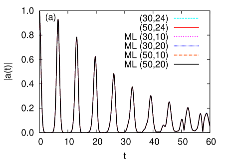
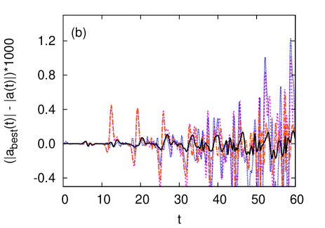
Results for the low ($\lambda=\lambda_{0}$) and high ($\lambda=2\lambda_{0}$) coupling regimes are shown in Figs. 2 and 3, respectively, where the absolute value of $a(t)$ is displayed. In both Figs. 2 and 3, the numbers in parenthesis correspond to $(N_{1},N_{2})$ in the trees in Fig. 1. For MCTDH $N_{2}$ equals the number of grid points and is given only for completeness. In the case of low coupling (Fig. 2), all calculations yield almost indistinguishable autocorrelation functions. Fig. 2b displays the difference between autocorrelation functions of the ML-MCTDH calculations and the best converged (50,24) MCTDH calculation. The (50,20) ML-MCTDH calculation is very close to the reference MCTDH result. The calculations that diverge earlier with respect to the reference result are the (30,10) and (50,10) ones due a poorer convergence of the lower layer, while the ML-MCTDH (30,20) calculation starts to deviate from the reference result after the system has completed five to six oscillation cycles.

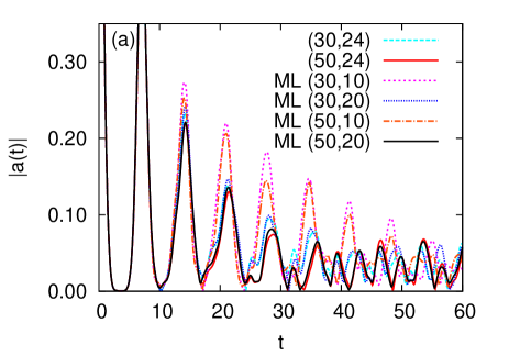
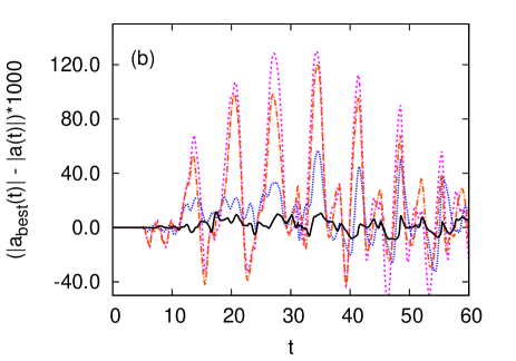
After doubling the strength of the coupling parameter, the situation becomes more complex. In Fig. 3a one sees that after two oscillation periods the autocorrelation functions of the different propagations start to diverge on an appreciable scale. Only the best MCTDH calculation (50,24), and the best ML-MCTDH (50,20) result in very close autocorrelations up to 60 time units. Fig. 3b shows the difference between the ML-MCTDH results and the (50,24) MCTDH calculation. The two worst calculations are clearly the ones with $N_{2}=10$. In this case, the correlation at the lowest layer, i.e. between DOF $(q_{1},q_{2})$, $(q_{3},q_{4})$ and $(q_{4},q_{5})$ is not well represented. It is important to note that the (50,10) calculation does not offer an improvement over the (30,10) one. The missing correlation within the logical coordinates in the lowest layer cannot be regained by having more SPFs in higher layers. Similarly as in standard MCTDH calculations, the eigenvalues of the density matrices at each layer, the natural populations (NP), provide an indication of the degree of convergence of a calculation. As a rule of thumb, the smallest NP should be of the order of $10^{-5}$ to provide good results in many cases, although this can vary depending on what quantity one is trying to compute. For the (50,10) and (50,20) ML-MCTDH calculations at $t=60$, the smallest NP of the three logical coordinates at the top layer are $(1.4\cdot 10^{-5}\,/\,1.3\cdot 10^{-4}\,/\,9.3\cdot 10^{-5})$ and $(3.4\cdot 10^{-5}\,/\,1.8\cdot 10^{-4}\,/\,1.3\cdot 10^{-4})$, respectively. Therefore, the convergence at the top layer is slightly worse for the (50,20) case than for the (50,10) case, even though by comparison to the standard MCTDH calculation it is clear that the (50,20) calculation provides better converged results than the (50,10). Hence, by allowing more SPFs at the second layer, the evolution of the top layer SPFs becomes more complex since they have more variational freedom.

As a remark to the 6D simulations, in this case standard MCTDH calculations are more efficient than ML-MCTDH ones. Only in the case of having a larger number of DVR points per degree of freedom resulting in very large 2D combined coordinates, would the introduction of a further layer (compare Figs. 1a and 1b) constitute an advantage. Efficiency issues are discussed later in relation to the larger HH simulations and to pyrazine.

III.1.2 18D simulations

FIGURE 4 AROUND HERE

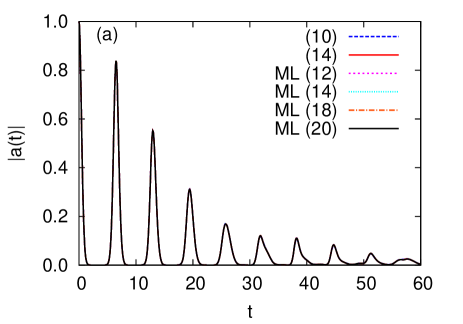
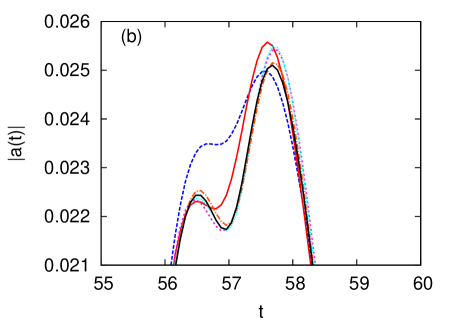
Next we discuss simulations on a 18D HH model with $\lambda=\lambda_{0}$. The initial wavepacket is centered at $q_{\kappa}=2$ for coordinates $q_{4}$, $q_{8}$, $q_{12}$ and $q_{16}$, resulting in an initial energy of $15.807$. As in the 6D case, wavepackets are propagated up to 30 time units. For this model we run standard MCTDH calculations in which the 18 physical coordinates are grouped into 6 combined modes (logical coordinates) with three primitive DOFs each. The tree representation of the MCTDH wavefunction is given in Fig. 4a. There, $N_{1}$ is the number of SPFs per combined mode and $N_{2}=24$ is the number of DVR functions per DOF. Two standard MCTDH calculations were performed, using $N_{1}=10$ and $N_{1}=14$ SPFs per combined mode, resulting in $10^{6}$ and $7.5\cdot 10^{6}$ configurations, respectively. ML-MCTDH calculations based on the tree structure in Fig. 4b and using the same Hamiltonian and initial conditions were performed as well. In the ML calculations various basis sizes were employed, always keeping $N_{1}$ equal to $N_{2}$. The autocorrelation functions resulting from the MCTDH and ML-MCTDH calculations are presented in Fig. 5, where the numbers in the legend correspond to $N_{1}$ for MCTDH, and to $N_{1}$ and $N_{2}$ for ML-MCTDH. At the scale shown in Fig. 5a all simulations yield very similar results. Fig. 5b shows the last revival of $|a(t)|$ in more detail. The worst result appears to be the standard MCTDH calculation with $N_{1}=10$. The various ML-MCTDH calculations approach the $(N_{1},N_{2})=20$ result as the size of the basis increases, while the standard MCTDH with $N_{1}=14$ seems not to be yet be fully converged with respect to the trend of the ML-MCTDH simulations.

FIGURE 5 AROUND HERE

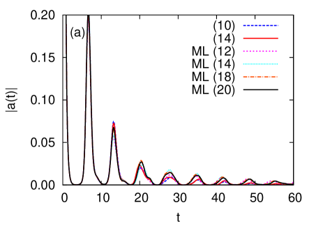
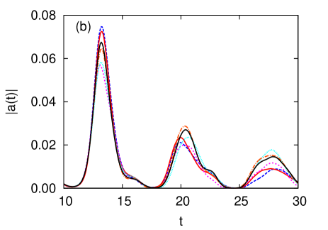
The set of simulations described above were repeated doubling coupling parameter $\lambda=2\lambda_{0}$. For this coupling strength the revivals of the autocorrelation function decay after a few oscillations. The different simulations yield still similar autocorrelation functions (Fig. 6a), but differences are now larger than in the small coupling parameter case, which can be seen by inspecting Fig. 6b. There, the autocorrelation function between 10 and 30 time units is shown in detail, and after this time the autocorrelation has almost vanished. By looking at the autocorrelation functions of the various MCTDH and ML-MCTDH simulations one sees that full convergence with respect to the number of SPFs has not been completely reached, even at short propagation times. Full convergence of the 18D HH model with a coupling parameter of $\lambda=2\lambda_{0}$ is a very demanding task. The $N_{1}=14$ MCTDH simulation was run on 8 processors using shared-memory parallelization, for which a speed factor of about 3 can be expected . Such calculation required 71 hours of wall clock time on the 8 processors and would have taken about 200 hours on a single processor. About 5 GB of main memory were used for the wavepacket propagation. In contrast to this, the largest ML-MCTDH calculation with $(N_{1},N_{2})=20$ required 136 hours of wall-clock time running on a single processor and the wavepacket propagation used less than 500 MB of main memory, while the $(N_{1},N_{2})=12$ ML-MCTDH calculation needed only 7 hours on a single processor. All calculations reported in this paper are performed on an quad-core Opteron, processor type 2384, 2.7 GHz.

FIGURE 6 AROUND HERE

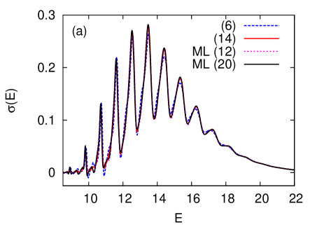
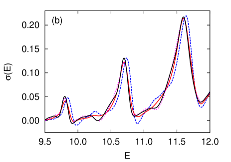
If we now look at the spectra of the propagated wavepackets obtained by Fourier Transform (FT) of the corresponding autocorrelation functions we see that they are very similar. The spectra of two MCTDH calculations with $N_{1}=6$ and $N_{1}=14$ are shown in Fig. 7. The $N_{1}=10$ case (not shown) yields a spectrum very similar to the larger MCTDH calculation. The spectra of two ML-MCTDH calculations are also presented in Fig. 7, namely the smallest and largest calculations of the ML series. The spectrum of the MCTDH calculation with $N_{1}=6$ yields somewhat different intensities in the higher energy range than the other simulations. When closely inspecting the lower energy range (Fig. 7b) one finds a non-negligible energy shift of the spectrum of the small MCTDH calculation to higher energies. Interestingly, the $N_{1}=6$ standard MCTDH propagation required 17 hours running on 8 parallel processors in the same conditions as discussed above. The number of SPFs for this simulation was chosen such that the cost would be comparable to that of the smaller $(N_{1},N_{2})=12$ ML-MCTDH calculation. The smaller ML-MCTDH calculation required 7 hours of wall-clock time on a single CPU running on the same hardware, and its spectrum is already very similar to the spectra of the larger MCTDH and ML-MCTDH calculations.

FIGURE 7 AROUND HERE

The size of the 18D HH model is such that standard MCTDH calculations can still be conducted to a good accuracy. Contrary to the 6D case however, for this dimensionality it already pays off to introduce a further layer in the calculation, and 3-layer ML calculations offer results of similar quality than the standard MCTDH ones with a noticeably smaller cost.

III.1.3 1458D simulations

Finally, we report ML-MCTDH simulations on a HH model with 1458 DOF and coupling constant $\lambda=\lambda_{0}$. The system is described in this case by a 7-layer wavefunction. At the top level the coordinates are divided in three groups of 486 coordinates, which are subsequently divided again in three groups, and so on. This is repeated until groups of two primitive DOF are reached in the seventh layer, which are then kept combined. For this deeply layered wavefunction two limiting cases are numerically investigated. In example (1), DOF $q_{486}$ and $q_{487}$ are displaced for $t=0$ such that $\langle q_{\kappa}\rangle=2$. Since the two degrees of freedom are adjacent, there is a coupling term in the Hamiltonian between them. However, $q_{486}$ and $q_{487}$ belong to different logical coordinates at all layers of the tree. They belong to logical coordinates $Q^{1}_{1}$ and $Q^{1}_{2}$ at the top layer and to coordinates $Q^{6;1,3,3,3,3}_{3}$ and $Q^{6;2,1,1,1,1}_{1}$ at the bottom layer, respectively. In example (2), DOF $q_{729}$ and $q_{730}$ are initially set at $\langle q_{\kappa}\rangle=2$. Again, these two DOF are coupled in the Hamiltonian, but in this case they belong to the same logical coordinate at all levels, starting from logical coordinate $Q^{1}_{2}$ at the top layer and down to the same combined mode $Q^{6;2,2,2,2,2}_{2}$ at the bottom layer. In both cases, decoupled reference calculations are also conducted in which the coupling term between DOF $q_{486}$ and $q_{487}$ for case (1) and between DOF $q_{729}$ and $q_{730}$ for case (2) are eliminated from the Hamiltonian. The simulated system corresponds to a long chain of coupled oscillators. In both cases (1) and (2), the initially displaced degrees of freedom are far from the ends of the chain. Therefore the system dynamics in both cases should be very similar, since the extremes of the chain will play a role only at much longer times than simulated.

FIGURE 8 AROUND HERE

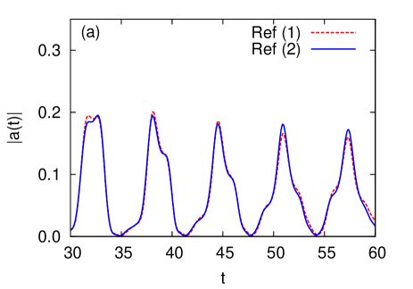
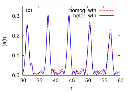
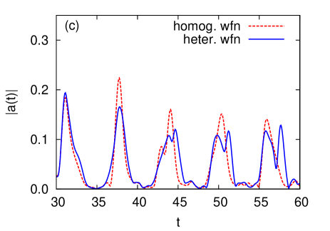
Fig. 8a shows the autocorrelation function of the two decoupled reference calculations. In both cases the wavefunction consists of 5 SPFs for each logical coordinate at all layers, which results in $2\,326\,520$ TD coefficients. Since there is no coupling term in the Hamiltonian between the two initially displaced DOF, their distance along the tree structure should be irrelevant, and in fact both simulations yield nearly identical results. When the interaction is turned on, however, the distance between two coupled DOF along the tree does matter. In case (2) the tree distance between DOF $q_{729}$ and $q_{730}$ is the shortest possible. Fig. 8b shows the autocorrelation of two propagations for case (2). One of them is based on the same wavefunction as the reference results. A second propagation is based on a wavefunction with 20 SPFs for the combined mode containing $q_{729}$ and $q_{730}$, $Q^{6;2,2,2,2,2}_{2}$, and 15 SPFs for the two neighboring combined modes $Q^{6;2,2,2,2,2}_{1}$ and $Q^{6;2,2,2,2,2}_{3}$. One layer above the wavefunction has 10 SPFs for logical coordinates $Q^{5;2,2,2,2}_{2}$ and its two neighbors $Q^{5;2,2,2,2}_{1}$ and $Q^{5;2,2,2,2}_{3}$. Further up in the tree, logical coordinates containing $q_{729}$ and $q_{730}$ and its two neighbor coordinates have 7 SPFs each. All other logical coordinates at all layers are represented by 4 SPFs. This scheme results in $1\,853\,310$ TD coefficients. As seen in Fig. 8b, both wavefunctions yield very similar autocorrelations until the end of the simulation. By inspecting the natural populations at the final time for both case (2) simulations one notices however that the convergence at the lowest layer is rather poor for the homogeneous wavefunction with 5 SPFs overall, with a population of the order of $10^{-2}$ for the last natural orbital of coordinate $Q^{6;2,2,2,2,2}_{2}$. When inspecting the populations of the propagation with more SPFs for logical coordinates close to the displaced mode $Q^{6;2,2,2,2,2}_{2}$, substantially improved values of at least $10^{-4}$ are obtained for all logical coordinates containing $Q^{6;2,2,2,2,2}_{2}$ at all levels.

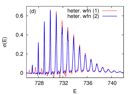
Example (1), in which the distance between both initially displaced DOF $q_{486}$ and $q_{487}$ is the largest possible within the tree, has a different convergence behavior. Fig. 8c compares two autocorrelations for case (1). A first propagation is based in the same homogeneous wavefunction already discussed for case (2). A second simulation is based on a wavefunction with 15 SPFs for logical coordinates $Q^{6;1,3,3,3,3}_{3}$ and $Q^{6;2,1,1,1,1}_{1}$, which respectively contain DOF $q_{486}$ and $q_{487}$, and with 7 SPFs for logical coordinates containing also $q_{486}$ and $q_{487}$ at all layers. All other logical coordinates have 4 SPFs and total number of TD coefficients is now $1\,810\,940$. Now, both autocorrelations start to diverge after about 30 time units, and they also start to diverge from the autocorrelations of case (2) after about the same propagation time. Interestingly however, the least populated natural orbitals for logical coordinates $Q^{6;1,3,3,3,3}_{3}$ and $Q^{6;2,1,1,1,1}_{1}$ have populations of the order of $10^{-3}$ to $10^{-4}$, and this is substantially improved to $10^{-4}$ to $10^{-5}$ for the non-homogeneous wavefunction. All other natural populations in the whole tree structure, for both wavefunctions, remain in the order of $10^{-4}$ or below. The spectra of cases (1) and (2) for the non homogeneous wavefunctions (Fig. 8d) agree to each other rather well. The differences in the autocorrelations are however reflected in a appearance of a few spurious lines with low intensity in the low energy part of the spectrum for case (1).

The analysis of case (2) indicates that when correlated DOF are close to each other in the tree structure, i.e. they are connected in the deeper layers of the tree, it is easy to achieve convergence by increasing the number of SPFs close to such DOF in the tree structure. Even most importantly, one can expect an early convergence to the correct trend, since even with not very good natural populations at low layers the results are already correct. Case (1), on the contrary, is an example of the wrong choice of tree structure. Even with natural populations smaller than case (2) for the homogeneous wavefunction, and populations of the order of $10^{-4}$ in most layers, the results are different from case (2) and also differ between the two different wavefunctions tried for case (1). In case (1) a general and substantial increase of SPFs for the whole tree structure would probably be needed to obtain better converged results. The early convergence of the method with the number of SPFs appears to be damaged in case (1) in light of the difference in results of for the two different wavefunctions tried.

III.2 Pyrazine

We now turn our attention to the photophysics of pyrazine using the 24D second-order vibronic-coupling Hamiltonian of Raab et al. raa99:936 . In pyrazine, the spectrum obtained from excitation to the second excited electronic state $S_{2}$ presents a broad feature due to the fast decay of the system into the $S_{1}$ electronic state through a conical intersection. Such a decay occurs during a few ten fs after photoexcitation. Although obtaining the right position and approximate shape of the broad band is relatively straightforward and several different approaches can claim to have achieved it, reproducing the fine details of the absorption spectrum is quite hard, since a good quality propagation up to relatively long times is needed. Therefore, the 24D model of pyrazine in Ref. raa99:936 has often been used to benchmark different quantum dynamical approaches including semiclassical methods tho00:10282 , the multiple-spawning method ben02:439 , the coupled coherent state method sha04:3563 ; sha10:244111 , the matching-pursuit/split-operator Fourier-transform method che06:124313 , and the Gaussian-MCTDH method bur08:174104 .

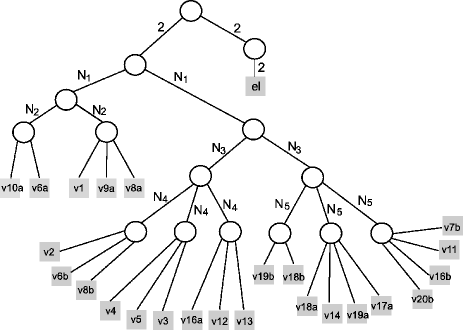
In the 24D simulations reported here, we use the same DVR and grid points as in the MCTDH simulations of Refs. raa99:936 and bur08:174104 . These MCTDH calculations were based on mode combination scheme in which the 24 primitive coordinates were grouped into the 8 combined modes $Q_{1}=[\nu_{10a},\nu_{6a}]$, $Q_{2}=[\nu_{1},\nu_{9a},\nu_{8a}]$, $Q_{3}=[\nu_{2},\nu_{6b},\nu_{8b}]$, $Q_{4}=[\nu_{4},\nu_{5},\nu_{3}]$, $Q_{5}=[\nu_{16a},\nu_{12},\nu_{13}]$, $Q_{6}=[\nu_{19b},\nu_{18b}]$, $Q_{7}=[\nu_{18a},\nu_{14},\nu_{19a},\nu_{17a}]$ and $Q_{8}=[\nu_{20b},\nu_{16b},\nu_{11},\nu_{7b}]$. A description of these vibrational modes is found in Ref. raa99:936 and it is beyond the purpose of this paper to reproduce their discussion here. All but one of the reported ML-MCTDH simulations are based on this set of combined modes, which are then grouped in the ML tree as depicted in Fig. 9. This makes the ML-MCTDH calculations numerically easier to compare to previous MCTDH calculations, for example when computing wavefunction overlaps, since the ML-MCTDH wavefunction can be easily expanded into the corresponding MCTDH form (if the expanded form is still of a manageable size) in a similar way as an MCTDH wavefunction can be expanded to a standard wavefunction on the primitive grid, Eq. (1). In the simulation named ML-MCTDH-1, however, we further divide modes $Q_{7}$ and $Q_{8}$, which contain coordinates with large primitive grids, in order to better exploit the capabilities of ML-MCTDH. We used $Q_{1}\cdots Q_{5}$ as above but: $Q_{6}=[\nu_{19b}]$, $Q_{7}=[\nu_{18b}]$, $Q_{8}=[\nu_{18a},\nu_{14}]$, $Q_{9}=[\nu_{19a},\nu_{17a}]$, $Q_{10}=[\nu_{16b}]$, and $Q_{11}=[\nu_{20b},\nu_{11},\nu_{7b}]$. This division is accomplished by adding a further (a sixth) layer to the tree depicted in Fig. 9.

FIGURE 9 AROUND HERE

For non-adiabatic systems with more than one electronic state MCTDH is often used in its multi-set formulation bec00:1 ; mey03:251 ; mey09:book , in which different sets of SPFs are used for each electronic DOF. All pyrazine MCTDH calculations discussed here were done using the multi-set formalism. In the multi-set formalism the SPFs of each state are optimal for that state, so that a smaller number of SPFs per state are needed than in a single-set calculation. The computational cost grows exponentially with the product of SPFs in each state, but linearly with the number of SPFs in different electronic states, which makes multi-set calculations often advantageous with respect to single-set ones for the same system. In ML-MCTDH, a multi-set formulation would be extremely cumbersome because one would end up with several tree structures to be specified, one for each electronic state, and a much more complex algorithm. On the other hand, the favorable scaling of ML-MCTDH with the number of DOF makes it unnecessary to use a multi-set ML formulation. In simulations of non-adiabatic systems with ML-MCTDH the electronic DOF is hence just another coordinate that indexes the electronic states, as in usual single-set MCTDH calculations, and the ML-MCTDH algorithm remains unchanged. Consequently, in constructing the ML tree, one is free to group the electronic DOF in any convenient way with other coordinates and set it in any level of the tree where it may seem appropriate. For example, if only a subset of coordinates couple the different electronic states and the rest act as a bath, it may make sense to group the electronic DOF with the coordinates that control the non-adiabatic coupling, and then the system-bath separation can be placed one level above. In our simulations, the top layer contains coordinates ${Q_{vib},q_{el}}$, where $Q_{vib}$ groups the 24 vibrational modes of the system and $q_{el}$ denotes the electronic DOF. $Q_{vib}$ is further divided into two groups of coordinates, one containing modes ${\nu_{10a},\nu_{6a},\nu_{1},\nu_{9a},\nu_{8a}}$ and the other one containing the rest of modes. Modes ${\nu_{10a},\nu_{6a},\nu_{1},\nu_{9a}}$ define the ”system” in 4D models of pyrazine raa99:936 , while the rest have been usually termed ”bath” modes. Therefore, the first branching of the tree after separating electronic and vibrational coordinates can be understood as a system-bath separation. The resulting system and bath coordinates are further divided until modes of a manageable size are reached, as seen in Fig. 9.

TABLE 1 AROUND HERE

Table 1 presents some results for a set of ML-MCTDH simulations and three different MCTDH reference calculations. The calculation named here MCTDH-1 was reported in Ref. raa99:936 . The MCTDH-2 result was an MCTDH reference calculation in Ref. bur08:174104 , while the MCTDH-3 calculation is a new reference result for this system and corresponds to the largest MCTDH calculation reported for pyrazine to date. All simulations were run up to a propagation time of 150 fs.

FIGURE 10 AROUND HERE

FIGURE 11 AROUND HERE

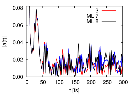
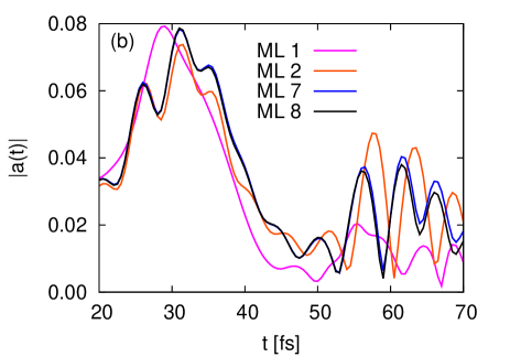
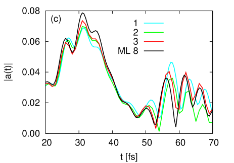
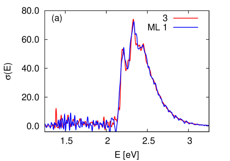
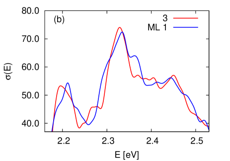
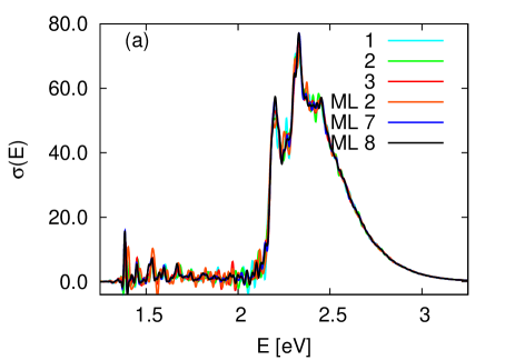
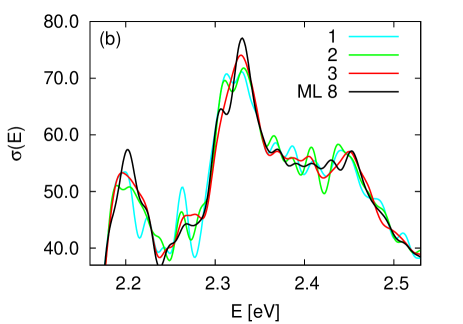
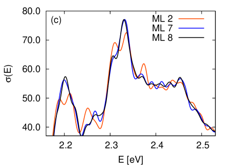
Fig. 10 presents the absolute value of the autocorrelation function for the ML-MCTDH and MCTDH calculations in Table 1. As in the HH cases above, the autocorrelation is computed using the relation for real initial states and symmetric Hamiltonians $a(t)=\langle\Psi^{*}(t/2)|\Psi(t/2)\rangle$. In Fig. 10b one sees that the ML-MCTDH-1 simulation presents severe deficiencies in $|a(t)|$, only following the general shape of the initial decay and the small revivals between 25 and 45 fs. This simulation is however extremely fast, needing only 7 minutes to run and consuming an incredibly small amount of resources. Regarding peak positions and intensities, the general features of the spectrum in Fig. 11a, although not too accurate, are there. The details of the peaks below 2.1 eV are not reproduced and the high energy tail, above 2.5 eV, shows an artificial oscillatory behavior. But beside this, the main peak is amazingly well reproduced, considering the inexpensiveness of the calculation. The larger ML-MCTDH-2 simulation, needing 33 hours (five times faster than the MCTDH-1 reference result), already presents the correct trends in the autocorrelation function up to 70 fs, resulting in a much improved spectrum (Figs. 12a and 12c). The autocorrelations of the two most accurate ML-MCTDH simulations present features that resemble closely those of the most accurate MCTDH result. In fact, when comparing the various structures of $|a(t)|$ in Fig. 10c, the tendency of the MCTDH-1, -2, and -3 simulations is towards the ML-MCTDH-8 simulation, which seems to indicate that the best ML-MCTDH results are better converged than the best MCTDH run. This can be seen in the height of the structure between 30 and 40 fs, and also in the position of the three peak structures between 55 and 70 fs. When turning to the spectra in Fig. 12, similar conclusions can be drawn, for example examining closely the peaks at 2.2 and 2.35 eV in Fig. 12b. It is remarkable that simulation ML-MCTDH-7, which seems to be already better converged than the best MCTDH result reported, required about 25% of runtime and 1% of memory (in terms of wavefunction size) than the latter.

FIGURE 12 AROUND HERE

In terms of efficiency, the second column in Table 1 contains the wall-clock time of each calculation. All ML-MCTDH calculations were run on a single-processor, so CPU time equals in this case wall-clock time, and used the variable mean-field (VMF) bec00:1 propagation scheme. The MCTDH calculations were run using the shared-memory parallelized MCTDH code bri08:141 ; bri09:67 and 8 processors in parallel, using the constant mean-field (CMF) propagation scheme. bec97:113 ; bec00:1 ; man06:168 The speed-up factor of the MCTDH parallel computations is 2.9, 3.3, and 3.7 for MCTDH-1, -2, and -3, respectively, and this factor has been already multiplied to the MCTDH wall-clock times, yielding the CPU time that would have been taken on a single CPU so that they can be readily compared to the ML-MCTDH values. These speed-up are reasonable but not particularly good, which is due to the relatively small Hamiltonian operator of the pyrazine model and better scalings have been obtained, e.g. for the Zundel cation H₅O${}_{2}^{+}$ bri08:141 ; bri09:67 ; bri10:147 . All calculations were run on the same machine and CPU type (see caption of Table 1). All reported simulations, including the HH ones but except for ML-1, were run with a rather high integrator precision of $10^{-7}$. This was done to exclude any numerical artifacts and to ensure that all discussed effects originate form various sizes of sets of SPFs. The fast but low-accuracy calculation ML-1 was run with an integrator precision of $10^{-5}$. Reducing the high integrator precision will speed-up the calculations by factors between 1.5 and 2 without introducing visible changes into the spectra.

The third column in Table 1 contains the total number of time-dependent coefficients in the wavefunction representation. Two aspects are remarkable here. First, ML-MCTDH wavefunctions are much more compact than MCTDH ones. Second, the CPU time divided by the number of coefficients is about one order of magnitude larger in ML-MCTDH, this factor remaining quite stable along the series of calculations. Therefore, integrating each coefficient in ML-MCTDH is harder than in MCTDH due to the natural overhead of the ML-MCTDH algorithm. However, this is compensated by the much smaller number of coefficients in the wavefunction. Such scaling effects become more and more pronounced with the size of the system, as was seen for the HH case, and ML-MCTDH propagations seem to become more efficient than MCTDH ones in terms of CPU time for systems larger than about 20 DOFs. Simulations ML-MCTDH-2 to -8 could be made even more efficient further dividing the largest combined modes at the lowest layer in a similar way as it was done for ML-MCTDH-1. Running on 8 processors, MCTDH-3 needed about 1000 hours to complete (unscaled wall-clock time), keeping up with the wall-clock time of the best ML-MCTDH calculations through parallelization. The MCTDH-3 calculation could in principle be made faster than ML-MCTDH using more hardware. However, for a molecular system doubling the size of pyrazine, a normal MCTDH calculation would be probably not doable, or at least not with a reasonable SPF basis size. On the contrary, that case would require an additional layer in a ML-MCTDH calculation, and the CPU cost would scale approximately linearly, rendering the simulation still doable. Regarding the different approaches tried on the pyrazine Hamiltonian over the years, ML-MCTDH offers by far the best quality/cost relation. The ML-MCTDH-2 simulation, which is already of a reasonable quality, takes about one day on a single CPU using little resources. The various ML-MCTDH simulations on the cheaper end yield spectra of a quality that other approaches hardly reach ben02:439 ; sha04:3563 or reach only by using a much larger amount of CPU and memory resources che06:124313 ; bur08:174104 . And again, accepting slightly larger deviations in the spectrum, an ML-MCTDH calculation on pyrazine takes only 7 minutes.

IV Summary and Conclusion

We presented the implementation of the ML-MCTDH approach into the Heidelberg MCTDH package, which is based on the recursive algorithm proposed by Manthe. A discussion of the concept of multilayer was given, and the working equations were provided making emphasis on the key points of the approach. For a comprehensive derivation of the working scheme one should see Ref man08:164116 . The use of the separable terms in the Hamiltonian in the recursive construction of the $h$-matrices and mean-fields at the different layers was discussed here with some detail.

The implementation, numerical performance, and general features of the ML-MCTDH approach have been tested by running simulations on the Henon-Heiles model and on pyrazine. For Henon-Heiles, simulations for the 6D, 18D and a large 1458D case have been reported. In the 6D and 18D cases, normal MCTDH calculations are performed for identical parameter sets for comparison, and for the 6D case MCTDH is more efficient than ML-MCTDH. The situation already changes for the 18D simulations, in which ML-MCTDH outperforms MCTDH. With respect to the natural populations, which are often used as a convergence criterion in MCTDH calculations, it is observed that when increasing the number of SPFs at lower layers for a given number of SPFs at higher layers, the convergence of the higher layer becomes worse although the overall quality may improve. This is due to the fact that the dynamics at the higher layers becomes more complex after increasing the size of the basis below. Hence, with respect to convergence, all layers have to be monitored when changing the basis size in some other layer.

For pyrazine, we test ML-MCTDH on the second-order vibronic-coupling Hamiltonian of Raab et. al, which has been used in testing several quantum dynamical methods. By properly choosing the tree scheme, we report a ML-MCTDH simulation that takes only 7 minutes of CPU time in one processor and very few memory, and that recovers the main spectral features reasonably well. On the other hand, we report ML-MCTDH simulations which are converged to at least the same degree as the best reference MCTDH results available, taking only 25% of the CPU time and 1% of wavefunction storage space with respect to such reference results. As seen in the pyrazine case, ML-MCTDH allows for a consistent separation of the degrees of freedom considered as system and the ones considered as bath, providing the variationally optimal system-bath evolution for the particular selection of the basis size and the layering scheme. By using ML-MCTDH for system-bath problems, schemes that simplify the system-bath ansatz lop10:104103 or schemes that reduce a larger bath to a subset of effective modes gin06:144103 , become unnecessary.

ML-MCTDH is an efficient tool for model systems, which had already been demonstrated by works of Wang and Thoss. ML-MCTDH has been shown here to be a very powerful tool to treat more realistic molecular Hamiltonians as well. The fact that a tree structure needs to be chosen, often based on intuition or experience, and that convergence has to be monitored at the different layers, makes its use less straightforward than MCTDH. Therefore, some work in the direction of automating certain decisions regarding the tree structure will have to be carried on. Regarding efficiency, it will be interesting to develop good dedicated constant mean-field (CMF) propagation schemes bec97:113 ; bec00:1 ; man06:168 for the ML case. And, of course, parallelizing the ML-code will be an important step, as ML-MCTDH is for treating large systems. Beyond applications of ML-MCTDH to problems involving nuclear dynamics, for which it has certainly a large potential, new directions will have to be explored in the future. We believe that methods based on or taking advantage of the ML-MCTDH concept can be useful in a wide range of situations. For example, we envisage that in simulations of mixtures of different kinds of particles (different kinds of fermions and bosons, electrons and nuclei in molecules, etc.), the different types of particles can be separated and correlated to each other at the top layer, while the internal dynamics of each group takes place in the layers below. ML-MCTDH constitutes a consistent and powerful tool for the quantum-dynamical description of high dimensional molecular systems. This and other kinds of challenging applications remain the subject of future investigations.

V Acknowledgments

Financial support by the Deutsche Forschungsgemeinschaft (DFG) is gratefully acknowledged.

Table 1: Simulation parameters of the various MCTDH and ML-MCTDH 24D pyrazine calculations. The second column contains the wall-clock time of each simulation. ML-MCTDH calculations were run on a single CPU, so that the wall-clock time equals the CPU time. The MCTDH calculations were run on 8 CPUs using shared-memory parallelization bri08:141 ; bri09:67 . The speed-up factor of the 8-processor parallel pyrazine calculations is 2.9, 3.3 and 3.7 for the MCTDH-1, -2 and -3 cases, respectively. The wall-clock times given for the MCTDH reference results are already scaled up by the corresponding speed-up factor and therefore reflect the time that such simulation would have taken on a single processor. Therefore they can be readily compared to the ML-MCTDH values. All simulations were run on the same machine and CPU type, namely Quad-Core AMD Opterons, processor type 2384 running at 2.7 GHz. The third column shows the total number of time-dependent coefficients propagated in each case. The fourth column contains, for ML-MCTDH simulations, the number of SPFs for each node of the tree according to the representation in Fig. 9. The parenthesis indicate that different $N_{5}$ values were taken for each of the branches. The asterisk for the ML-1 case indicates that there is a further layer below the branches corresponding to $N_{5}$ (See text and Fig. 9 for details). For the MCTDH calculations, the fourth column contains in each parenthesis the number of SPFs for combined modes $Q_{1}$ to $Q_{8}$ for electronic states $S_{1}$ and $S_{2}$, respectively. All reported simulations, except for ML-1, were run with a rather high integrator precision of $10^{-7}$. (See text). ML-1 was run with $10^{-5}$. Reducing the high integrator precision will speed-up the calculations by factors between 1.5 and 2 without introducing visiable changes into the spectra.

Simulation CPU time [h:m] tot. coef [$N_{1}$,$N_{2}$,$N_{3}$,$N_{4}$,$N_{5}$] ML-1 0:07 $22\,444$ [$4,4,3,2,(3,2,2)^{*}$] ML-2 33:48 $206\,660$ [$12,13,10,8,8$] ML-3 57:12 $238\,054$ [$14,14,11,8,(12,8,8)$] ML-4 113:54 $294\,820$ [$16,16,13,10,(13,10,10)$] ML-5 135:31 $288\,324$ [$25,25,11,8,(12,8,8)$] ML-6 252:31 $337\,408$ [$25,25,13,10,(13,10,10)$] ML-7 725:29 $456\,584$ [$30,30,18,12,(15,12,13)$] ML-8 1123:38 $512\,560$ [$32,32,21,12,(17,12,14)$] [$(n_{1}^{S_{1}},n_{1}^{S_{2}}),\ldots,(n_{8}^{S_{1}},n_{8}^{S_{2}})$] MCTDH-1 155:58 $3\,029\,424$ [$(14,11),(8,7),(6,5),(6,4),(4,5),(7,7),(5,5),(3,4)$] MCTDH-2 629:58 $11\,282\,152$ [$(19,12),(10,7),(5,4),(7,4),(5,3),(11,9),(7,5),(4,4)$] MCTDH-3 3721:40 $46\,351\,392$ [$(21,15),(12,8),(7,6),(8,5),(7,5),(12,10),(7,5),(5,5)$]

Figure Captions

Figure 1: Tree structures for the MCTDH and ML-MCTDH wavefunctions of the 6D Henon-Heiles simulations. (a) MCTDH wavefunction tree, in which the coordinates are combined in groups of two. $N_{2}$ refers in this particular case to the number of primitive basis functions or grid points. (b) ML-MCTDH wavefunction tree. This tree is similar to the MCTDH tree, but the three combined modes have been separated by adding an extra layer. For the ML-MCTDH wavefunction $N_{3}$ corresponds now the number of primitive basis functions and for $N_{2}\equiv N_{3}$ (and same $N_{1}$) the ML-MCTDH case becomes numerically identical to the MCTDH one.

Figure 2: (color) (a) Absolute value of the autocorrelation function for various MCTDH and ML-MCTDH 6D Henon-Heiles simulations with a coupling parameter $\lambda=\lambda_{0}$. The numbers in parenthesis correspond to ($N_{1},N_{2}$) in Fig. 1. In the key, plain numbers indicate MCTDH calculations and the symbol ML designates ML-MCTDH calculations. (b) Difference between the autocorrelations of the ML-MCTDH simulations and the (50,24) MCTDH calculation.

Figure 3: (color) (a) Absolute value of the autocorrelation function for various MCTDH and ML-MCTDH 6D Henon-Heiles simulations with a coupling parameter $\lambda=2\lambda_{0}$. The numbers in parenthesis correspond to ($N_{1},N_{2}$) in Fig. 1. (b) Difference between the autocorrelations of the ML-MCTDH simulations and the (50,24) MCTDH calculation. In the key, ML is for ML-MCTDH.

Figure 4: Tree structures for the MCTDH and ML-MCTDH wavefunctions of the 18D Henon-Heiles simulations. The MCTDH wavefunction (a) consists of six combined modes, each of them grouping three primitive coordinates. The ML-MCTDH wavefunction (b) starts dividing the system in three logical coordinates, and each of them is further divided in three combined modes. The resulting tree has three layers of TD coefficients.

Figure 5: (color) (a) Absolute value of the autocorrelation function for various MCTDH and ML-MCTDH 18D Henon-Heiles simulations with a coupling parameter $\lambda=\lambda_{0}$. For the MCTDH cases the number in parenthesis refers to $N_{1}$ in Fig. 4a. For the ML-MCTDH cases the number in parenthesis refers to $N_{1}$ and $N_{2}$ in Fig. 4b, which are set equal in the reported simulations. (b) Detailed view of the last recurrence structure between 55 and 60 time units. In the key, ML is for ML-MCTDH.

Figure 6: (color) (a) Absolute value of the autocorrelation function for various MCTDH and ML-MCTDH 18D Henon-Heiles simulations with a coupling parameter $\lambda=2\lambda_{0}$. For the MCTDH cases the number in parenthesis refers to $N_{1}$ in Fig. 4a. For the ML-MCTDH cases the number in parenthesis refers to $N_{1}$ and $N_{2}$ in Fig. 4b, which are equal in the reported simulations. (b) Detailed view of the recurrence structures between 10 and 30 time units. In the key, ML is for ML-MCTDH.

Figure 7: (color) (a) Spectra for various MCTDH and ML-MCTDH 18D Henon-Heiles simulations with a coupling parameter of $\lambda=2\lambda_{0}$. The numbers in parenthesis have the same meanings as in Fig. 6. (b) Detailed view of the three first peaks between $6.2$ and $7.9$ energy units. In the key, ML is for ML-MCTDH. The spectra are obtained by a Fourier-transform of the autocorrelation function using a $cos^{2}$ filter bec00:1 ; mey09:book to minimize spurious effects known as Gibbs phenomenon.

Figure 8: (color) Absolute value of the autocorrelation of the ML-MCTDH 1458D Henon-Heiles simulations for time units 30 to 60. (a) Reference results without coupling term between the two displaced coordinates for case (1) (red dashed), in which the two initially displaced degrees of freedom belong to different logical coordinates at all layers, and case (2) (blue line), in which the two initially displaced degrees of freedom belong to the same logical coordinate at all layers. (b) For case (2), homogeneous wavefunction (red dashed) and non homogeneous wavefunction with more SPFs at low layers (blue line). (c) For case (1), homogeneous wavefunction (red dashed) and non homogeneous wavefunction (blue line). The pairs of autocorrelation functions presented in plots (b) and (c) are almost identical until about 15 time units, but the autocorrelation functions of case (1) and (2) start to differ already after 5 time units. These differences increase with time and can be inspected for the time interval 30 to 60 by comparing figure (b) with (c). (d) Spectra of the calculations with the non homogeneous wavefunctions for cases (1) and (2). The spectra are obtained by a Fourier-transform of the autocorrelation function using a $cos^{2}$ filter bec00:1 ; mey09:book to minimize spurious effects known as Gibbs phenomenon.

Figure 9: Tree structure used in most of the ML-MCTDH simulations of 24D pyrazine. The maximum depth of the tree is five layers, and the first one separates the 24 vibrational coordinates and the discrete electronic degree of freedom. The number of SPFs denoted $N_{4}$ need not be necessarily the same, and in fact in some of the ML-MCTDH simulations they are chosen to be different. The same is true for the three $N_{5}$’s, which can be different. For the fast ML-1 calculation a 6th layer was added, see text.

Figure 10: (color) Absolute value of the autocorrelation function for the 24D pyrazine calculations. The numeration of the calculations is consistent with Table 1. (a) Best MCTDH result and two best ML-MCTDH results from 0 to 300 fs. (b) Detailed view of the recurrences between 20 and 70 fs for all reported MCTDH simulations and the best ML-MCTDH simulation (b), and for the two worst and two best converged ML-MCTDH runs (c). In the key, ML is for ML-MCTDH.

Figure 11: (color) (a) Spectra of the fastest ML-MCTDH 24D pyrazine calculation ($2.2\times 10^{4}$ TD coeff., 7 min. of CPU) and the best reference MCTDH result ($4.6\times 10^{7}$ TD coeff., 2901 hours of CPU). (b) Detailed view of the energy domain between 2.1 and 2.6 eV. The spectra are obtained by a Fourier-transform of the autocorrelation function using a $cos^{2}$ filter bec00:1 ; mey09:book to minimize spurious effects known as Gibbs phenomenon. The numeration of the calculations is consistent with Table 1. In the key, ML is for ML-MCTDH.

Figure 12: (color) (a) Spectra of the three reference MCTDH simulations and three of the ML-MCTDH simulations, among them the two best results, for 24D pyrazine. The spectra are obtained by a Fourier-transform of the autocorrelation function using a $cos^{2}$ filter bec00:1 ; mey09:book to minimize spurious effects known as Gibbs phenomenon. The numeration of the calculations is consistent with Table 1. For the energy domain between 2.1 and 2.6 eV: (b) The three reference MCTDH calculations compared to the best ML-MCTDH result and (c) ML-MCTDH simulations 2, 7 and 8. In the key, ML is for ML-MCTDH.

Figure 1: Vendrell and Meyer, Journal of Chemical Physics

Figure 2: Vendrell and Meyer, Journal of Chemical Physics

Figure 3: Vendrell and Meyer, Journal of Chemical Physics

Figure 4: Vendrell and Meyer, Journal of Chemical Physics

Figure 5: Vendrell and Meyer, Journal of Chemical Physics

Figure 6: Vendrell and Meyer, Journal of Chemical Physics

Figure 7: Vendrell and Meyer, Journal of Chemical Physics

Figure 8: Vendrell and Meyer, Journal of Chemical Physics

Figure 9: Vendrell and Meyer, Journal of Chemical Physics

Figure 10: Vendrell and Meyer, Journal of Chemical Physics

Figure 11: Vendrell and Meyer, Journal of Chemical Physics

Figure 12: Vendrell and Meyer, Journal of Chemical Physics

References

- (1) H.-D. Meyer, U. Manthe, and L. S. Cederbaum, Chem. Phys. Lett. 165, 73 (1990).
- (2) U. Manthe, H.-D. Meyer, and L. S. Cederbaum, J. Chem. Phys. 97, 3199 (1992).
- (3) M. H. Beck, A. Jäckle, G. A. Worth, and H.-D. Meyer, Phys. Rep 324, 1 (2000).
- (4) H.-D. Meyer and G. A. Worth, Theor. Chem. Acc. 109, 251 (2003).
- (5) H.-D. Meyer, F. Gatti, and G. A. Worth, editors, Multidimensional Quantum Dynamics: MCTDH Theory and Applications, Wiley-VCH, Weinheim, 2009.
- (6) A. Raab, G. Worth, H.-D. Meyer, and L. S. Cederbaum, J. Chem. Phys. 110, 936 (1999).
- (7) A. Markmann, G. Worth, S. Mahapatra, H.-D. Meyer, H. Köppel, and L. Cederbaum, J. Chem. Phys. 123, 204310 (2005).
- (8) L. J. Doriol, F. Gatti, C. Iung, and H.-D. Meyer, J. Chem. Phys. 129, 224109 (2008).
- (9) G. A. Worth, H.-D. Meyer, H. Köppel, and L. S. Cederbaum, Int. Rev. Phys. Chem. 27, 569 (2008).
- (10) O. Vendrell, F. Gatti, and H.-D. Meyer, J. Chem. Phys. 131, 034308 (2009).
- (11) F. Richter, P. Rosmus, F. Gatti, and H.-D. Meyer, J. Chem. Phys. 120, 6072 (2004).
- (12) C. Iung, F. Gatti, and H.-D. Meyer, J. Chem. Phys. 120, 6992 (2004).
- (13) S. Sukiasyan and H.-D. Meyer, J. Chem. Phys. 116, 10641 (2002).
- (14) F. Otto, F. Gatti, and H.-D. Meyer, J. Chem. Phys. 128, 064305 (2008).
- (15) T. Wu, H.-J. Werner, and U. Manthe, Science 306, 2227 (2004).
- (16) R. van Harrevelt, G. Nyman, and U. Manthe, J. Chem. Phys. 126, 084303 (2007).
- (17) S. Bhattacharya, A. N. Panda, and H.-D. Meyer, J. Chem. Phys. 132, 214304 (2010).
- (18) M.-C. Heitz and H.-D. Meyer, J. Chem. Phys. 114, 1382 (2001).
- (19) R. van Harrevelt and U. Manthe, J. Chem. Phys. 121, 3829 (2004).
- (20) C. Crespos, H.-D. Meyer, R. C. Mowrey, and G. J. Kroes, J. Chem. Phys. 124, 074706 (2006).
- (21) K. Sakmann, A. I. Streltsov, O. E. Alon, and L. S. Cederbaum, Phys. Rev. Lett. 103, 2206011 (2009).
- (22) O. E. Alon, A. I. Streltsov, and L. S. Cederbaum, Phys. Rev. A 373, 301 (2009).
- (23) S. Zöllner, H.-D. Meyer, and P. Schmelcher, Phys. Rev. Lett. 100, 040401 (2008).
- (24) T. B. J. Zanghellini, M. Kitzler and A. Scrinzi, J. Phys. B 37, 763 (2004).
- (25) G. Jordan and A. Scrinzi, New J. Phys. 10, 025035 (2008).
- (26) M. Nest, R. Padmanaban, and P. Saalfrank, J. Chem. Phys. 126, 214106 (2007).
- (27) S. Sukiasyan, C. McDonald, C. Destefani, M. Y. Ivanov, and T. Brabec, Phys. Rev. Lett. 102, 223002 (2009).
- (28) J. Zanghellini, M. Kitzler, C. Fabian, T. Brabec, and A. Scrinzi, Laser Phys. 13, 1064 (2003).
- (29) M. Nest, T. Klamroth, and P. Saalfrank, J. Chem. Phys. 122, 124102 (2005).
- (30) O. E. Alon, A. I. Streltsov, and L. S. Cederbaum, Phys. Rev. A 77, 033613 (2008).
- (31) H. Wang, J. Chem. Phys. 113, 9948 (2000).
- (32) M. Nest and H.-D. Meyer, J. Chem. Phys. 119, 24 (2003).
- (33) S. R. Chinnamsetty, M. Espig, B. N. Khoromskij, and W. Hackbusch, J. Chem. Phys. 127, 084110 (2007).
- (34) S. R. White and R. L. Martin, J. Chem. Phys. 110, 4127 (1999).
- (35) H. Wang and M. Thoss, J. Chem. Phys. 119, 1289 (2003).
- (36) H. Wang and M. Thoss, J. Chem. Phys. 124, 034114 (2006).
- (37) I. R. Craig, H. Wang, and M. Thoss, J. Chem. Phys. 127, 144503 (2007).
- (38) I. Kondov, M. Čížek, C. Benesch, H. Wang, and M. Thoss, J. Phys. Chem. C 111, 11970 (2007).
- (39) H. Wang and M. Thoss, New Journal of Physics 10, 115005 (2008).
- (40) H. Wang and M. Thoss, J. Chem. Phys. 131, 024114 (2009).
- (41) U. Manthe, J. Chem. Phys. 128, 164116 (2008).
- (42) U. Manthe, J. Chem. Phys. 130, 054109 (2009).
- (43) A. Jäckle and H.-D. Meyer, J. Chem. Phys. 104, 7974 (1996).
- (44) A. Jäckle and H.-D. Meyer, J. Chem. Phys. 109, 3772 (1998).
- (45) L. D. Lathauwer, B. D. Moor, and J. Vandewalle, SIAM Journal on Matrix Analysis and Applications 21, 1253 (2000).
- (46) L. D. Lathauwer, B. D. Moor, and J. Vandewalle, SIAM Journal on Matrix Analysis and Applications 21, 1324 (2000).
- (47) U. Manthe, J. Chem. Phys. 105, 6989 (1996).
- (48) M. Nest and H.-D. Meyer, J. Chem. Phys. 117, 10499 (2002).
- (49) M. Thoss, W. H. Miller, and G. Stock, J. Chem. Phys. 112, 10282 (2000).
- (50) M. Ben-Nun and T. J. Martínez, Adv. Chem. Phys. 121, 439 (2002).
- (51) D. V. Shalashilin and M. S. Child, J. Chem. Phys. 121, 3563 (2004).
- (52) D. Shalashilin, J. Chem. Phys. 132, 244111 (2010).
- (53) X. Chen and V. S. Batista, J. Chem. Phys. 125, 124313 (2006).
- (54) I. Burghardt, K. Giri, and G. A. Worth, J. Chem. Phys. 129, 174104 (2008).
- (55) M. Brill, O. Vendrell, F. Gatti, and H.-D. Meyer, Shared memory parallelisation of the multi-configuration time-dependent hartree method and application to the dynamics and spectroscopy of the protonated water-dimer, in High Performance Computing in Science and Engineering 07, edited by W. E. Nagel, D. B. Kröner, and M. Resch, pages 141–156, Heidelberg, 2008, Springer.
- (56) M. Brill, O. Vendrell, and H.-D. Meyer, Shared memory parallelization of the multiconfiguration time-dependent Hartree method and application to the dynamics and spectroscopy of the protonated water dimer, in Advances in the Theory of Atomic and Molecular Systems, edited by P. Piecuch, J. Maruani, G. Delgado-Barrio, and S. Wilson, volume 20, page 69, Springer Verlag, 2009.
- (57) M. H. Beck and H.-D. Meyer, Z. Phys. D 42, 113 (1997).
- (58) U. Manthe, Chem. Phys. 329, 168 (2006).
- (59) M. Brill, O. Vendrell, and H.-D. Meyer, Distributed memory parallelisation of the multi-configuration time-dependent hartree method, in High Performance Computing in Science and Engineering 09, edited by W. E. Nagel, D. B. Kröner, and M. Resch, pages 147–163, Heidelberg, 2010, Springer.
- (60) S. López-López and M. Nest, J. Chem. Phys. 132, 104103 (2010).
- (61) E. Gindensperger, I. Burghardt, and L. S. Cederbaum, J. Chem. Phys. 124, 144103 (2006).
Simulation CPU time [h:m] tot. coef [,,,,] ML-1 0:07 [] ML-2 33:48 [] ML-3 57:12 [] ML-4 113:54 [] ML-5 135:31 [] ML-6 252:31 [] ML-7 725:29 [] ML-8 1123:38 [] [] MCTDH-1 155:58 [] MCTDH-2 629:58 [] MCTDH-3 3721:40 []