Consistent Higher-Order Corrections to $\tilde{t}_{i}\to\tilde{b}_{j}H^{+}$ in the Complex MSSM

Abstract:

We review an analysis of a consistent renormalization of the top and bottom quark/squark sector of the MSSM with complex parameters (cMSSM). Various renormalization schemes are defined, analyzed analytically and tested numerically in the decays $\tilde{t}_{2}\to\tilde{b}_{i}\,H^{+}/W^{+}$ ($i=1,2$). No scheme is found that produces numerically acceptable results over all the cMSSM parameter space, where problems occur mostly already for real parameters. Some numerical examples for $\Gamma(\tilde{t}_{2}\to\tilde{b}_{1}H^{+})$ in our preferred scheme, “$m_{b},\,A_{b}$ $\overline{\mathrm{DR}}$” are shown.

1 Introduction

One of the main tasks of the LHC is to search for Supersymmetry (SUSY) [2]. The Minimal Supersymmetric Standard Model (MSSM) predicts two scalar partners for all Standard Model (SM) fermions as well as fermionic partners to all SM bosons. Of particular interest are the scalar partners of the heavy SM quarks, the scalar top quarks, $\tilde{t}_{i}$ ($i=1,2$) and scalar bottom quarks $\tilde{b}_{j}$ ($j=1,2$) due to their large Yukawa couplings. Depending on the SUSY mass patterns, possibly important decay modes of the scalar tops are,

$$\tilde{t}_{i}\to\tilde{b}_{j}H^{+}\quad(i,j=1,2)~{},$$ (1)

$$\tilde{t}_{i}\to\tilde{b}_{j}W^{+}\quad(i,j=1,2)~{},$$ (2)

where $H^{+}$ denotes the (positively) charged MSSM Higgs boson. These processes can constitute a large part of the total stop decay width, and, in case of decays to a Higgs boson, they can serve as a source of charged Higgs bosons in cascade decays at the LHC.

For a precise prediction of the partial decay widths corresponding to Eq. (1) and Eq. (2), at least the one-loop level contributions have to be taken into account. This in turn requires a renormalization of the relevant sectors, especially a simultaneous renormalization of the top and bottom quark/squark sector. Due to the $SU(2)_{L}$ invariance of the left-handed scalar top and bottom quarks, these two sectors cannot be treated independently. Within the framework of the MSSM with complex parameters (cMSSM) we review the analysis of various bottom quark/squark sector renormalization schemes [3], while for the top quark/squark sector a commonly used on-shell renormalization scheme is applied throughout all the investigations. An extensive list of earlier analyses and corresponding references can be found in Ref. [3]. The evaluation of the partial decay widths of the scalar top quarks are being implemented into the Fortran code FeynHiggs [4, 5, 6, 7].

2 The bottom/sbottom sector and its renormalization

2.1 The generic structure

The bilinear part of the Lagrangian with top and bottom squark fields, $\tilde{t}$ and $\tilde{b}$,

$${\cal L}_{\tilde{t}/\tilde{b}\text{ mass}} =-\begin{pmatrix}{{\tilde{t}}_{L}}^{\dagger},{{\tilde{t}}_{R}}^{\dagger}\end{pmatrix}{\mathbf{M}}_{\tilde{t}}\begin{pmatrix}{\tilde{t}}_{L}\\ {\tilde{t}}_{R}\end{pmatrix}-\begin{pmatrix}{{\tilde{b}}_{L}}^{\dagger},{{\tilde{b}}_{R}}^{\dagger}\end{pmatrix}{\mathbf{M}}_{\tilde{b}}\begin{pmatrix}{\tilde{b}}_{L}\\ {\tilde{b}}_{R}\end{pmatrix}~{},$$ (3)

contains the stop and sbottom mass matrices ${\mathbf{M}}_{\tilde{t}}$ and ${\mathbf{M}}_{\tilde{b}}$, given by

$${\mathbf{M}}_{\tilde{q}} =\begin{pmatrix}M_{\tilde{Q}_{L}}^{2}+m_{q}^{2}+M_{Z}^{2}c_{2\beta}(T_{q}^{3}-Q_{q}s_{\mathrm{w}}^{2})&m_{q}X_{q}^{*}\\[1.99997pt] m_{q}X_{q}&M_{\tilde{q}_{R}}^{2}+m_{q}^{2}+M_{Z}^{2}c_{2\beta}Q_{q}s_{\mathrm{w}}^{2}\end{pmatrix}$$ (4)

with $X_{q}=A_{q}-\mu^{*}\kappa$ and $\kappa=\{\cot\beta,\tan\beta\}$ for $q=\{t,b\}$. $M_{\tilde{Q}_{L}}^{2}$ and $M_{\tilde{q}_{R}}^{2}$ are the soft SUSY-breaking mass parameters. $m_{q}$ is the mass of the corresponding quark. $Q_{{q}}$ and $T_{q}^{3}$ denote the charge and the isospin of $q$, and $A_{q}$ is the trilinear soft SUSY-breaking parameter. The mass matrix can be diagonalized with the help of a unitary transformation ${{\mathbf{U}}}_{\tilde{q}}$,

$${\mathbf{D}}_{\tilde{q}} ={\mathbf{U}}_{\tilde{q}}\,{\mathbf{M}}_{\tilde{q}}\,{{\mathbf{U}}}_{\tilde{q}}^{\dagger}=\begin{pmatrix}m_{\tilde{q}_{1}}^{2}&0\\ 0&m_{\tilde{q}_{2}}^{2}\end{pmatrix}~{},\qquad{{\mathbf{U}}}_{\tilde{q}}=\begin{pmatrix}U_{\tilde{q}_{11}}&U_{\tilde{q}_{12}}\\ U_{\tilde{q}_{21}}&U_{\tilde{q}_{22}}\end{pmatrix}~{}.$$ (5)

The scalar quark masses, $m_{\tilde{q}_{1}}$ and $m_{\tilde{q}_{2}}$, will always be mass ordered, i.e. $m_{\tilde{q}_{1}}\leq m_{\tilde{q}_{2}}$:

$$m_{\tilde{q}_{1,2}}^{2} =\frac{1}{2}\left(M_{\tilde{Q}_{L}}^{2}+M_{\tilde{q}_{R}}^{2}\right)+m_{q}^{2}+\frac{1}{2}T_{q}^{3}M_{Z}^{2}c_{2\beta}$$

$$\quad\mp\frac{1}{2}\sqrt{\left[M_{\tilde{Q}_{L}}^{2}-M_{{\tilde{q}_{R}}}^{2}+M_{Z}^{2}c_{2\beta}(T_{q}^{3}-2Q_{q}s_{\mathrm{w}}^{2})\right]^{2}+4m_{q}^{2}|X_{q}|^{2}}~{}.$$ (6)

2.2 Renormalization of the bottom/sbottom sector

The field renormalization constants of the bottom/sbottom (as well as of the top/stop) sector are chosen according to an on-shell prescription [3].

The parameter renormalization can be performed as follows,

$${\mathbf{M}}_{\tilde{q}} \to{\mathbf{M}}_{\tilde{q}}+\delta{\mathbf{M}}_{\tilde{q}}$$ (7)

which means that the parameters in the mass matrix ${\mathbf{M}}_{\tilde{q}}$ are replaced by the renormalized parameters and a counterterm. After the expansion $\delta{\mathbf{M}}_{\tilde{q}}$ contains the counterterm part,

$$\delta{\mathbf{M}}_{\tilde{q}_{11}} =\delta M_{\tilde{Q}_{L}}^{2}+2m_{q}\delta m_{q}-M_{Z}^{2}c_{2\beta}\,Q_{q}\,\delta s_{\mathrm{w}}^{2}+(T_{q}^{3}-Q_{q}s_{\mathrm{w}}^{2})(c_{2\beta}\,\delta M_{Z}^{2}+M_{Z}^{2}\,\delta c_{2\beta})~{},$$ (8)

$$\delta{\mathbf{M}}_{\tilde{q}_{12}} =(A_{q}^{*}-\mu\kappa)\,\delta m_{q}+m_{q}(\delta A_{q}^{*}-\mu\,\delta\kappa-\kappa\,\delta\mu)~{},$$ (9)

$$\delta{\mathbf{M}}_{\tilde{q}_{21}} =\delta{\mathbf{M}}_{\tilde{q}_{12}}^{*}~{},$$ (10)

$$\delta{\mathbf{M}}_{\tilde{q}_{22}} =\delta M_{\tilde{q}_{R}}^{2}+2m_{q}\delta m_{q}+M_{Z}^{2}c_{2\beta}\,Q_{q}\,\delta s_{\mathrm{w}}^{2}+Q_{q}s_{\mathrm{w}}^{2}(c_{2\beta}\,\delta M_{Z}^{2}+M_{Z}^{2}\,\delta c_{2\beta})~{}.$$ (11)

Another possibility for the parameter renormalization is to start out with the physical parameters which corresponds to the replacement:

$${\mathbf{U}}_{\tilde{q}}\,{\mathbf{M}}_{\tilde{q}}\,{{\mathbf{U}}}_{\tilde{q}}^{\dagger} \to{\mathbf{U}}_{\tilde{q}}\,{\mathbf{M}}_{\tilde{q}}\,{{\mathbf{U}}}_{\tilde{q}}^{\dagger}+{\mathbf{U}}_{\tilde{q}}\,\delta{\mathbf{M}}_{\tilde{q}}\,{{\mathbf{U}}}_{\tilde{q}}^{\dagger}=\begin{pmatrix}m_{\tilde{q}_{1}}^{2}&Y_{q}\\ Y_{q}^{*}&m_{\tilde{q}_{2}}^{2}\end{pmatrix}+\begin{pmatrix}\delta m_{\tilde{q}_{1}}^{2}&\delta Y_{q}\\ \delta Y_{q}^{*}&\delta m_{\tilde{q}_{2}}^{2}\end{pmatrix}~{},$$ (12)

where $\delta m_{\tilde{q}_{1}}^{2}$ and $\delta m_{\tilde{q}_{2}}^{2}$ are the counterterms of the squark masses squared. $\delta Y_{q}$ is the counterterm to the squark mixing parameter $Y_{q}$ (which vanishes at tree level, $Y_{q}=0$, and corresponds to the off-diagonal entries in ${\mathbf{D}}_{\tilde{q}}={\mathbf{U}}_{\tilde{q}}\,{\mathbf{M}}_{\tilde{q}}\,{{\mathbf{U}}}_{\tilde{q}}^{\dagger}$, see Eq. (5)). Using Eq. (12) one can express $\delta{\mathbf{M}}_{\tilde{q}}$ by the counterterms $\delta m_{\tilde{q}_{1}}^{2}$, $\delta m_{\tilde{q}_{2}}^{2}$ and $\delta Y_{q}$. Especially for $\delta{\mathbf{M}}_{\tilde{q}_{12}}$ one yields

$$\delta{\mathbf{M}}_{{\tilde{q}}_{12}} =U^{*}_{\tilde{q}_{11}}U_{\tilde{q}_{12}}(\delta m_{\tilde{q}_{1}}^{2}-\delta m_{\tilde{q}_{2}}^{2})+U^{*}_{\tilde{q}_{11}}U_{\tilde{q}_{22}}\delta Y_{q}+U_{\tilde{q}_{12}}U^{*}_{\tilde{q}_{21}}\delta Y_{q}^{*}~{}.$$ (13)

For the top/stop sector we use an on-shell renormalization, see e.g. Refs. [9, 8, 3]. The various options to renormalize the bottom/sbottom sector are listed in Tab. 1.

scheme	$m_{\tilde{b}_{1,2}}$	$m_{b}$	$A_{b}$	$Y_{b}$	name
analogous to the $t/\tilde{t}$ sector: “OS”	OS	OS		OS	RS1
“$m_{b},\,A_{b}$ $\overline{\mathrm{DR}}$”	OS	$\overline{\mathrm{DR}}$	$\overline{\mathrm{DR}}$		RS2
“$m_{b},\,Y_{b}$ $\overline{\mathrm{DR}}$”	OS	$\overline{\mathrm{DR}}$		$\overline{\mathrm{DR}}$	RS3
“$m_{b}$ $\overline{\mathrm{DR}}$, $Y_{b}$ OS”	OS	$\overline{\mathrm{DR}}$		OS	RS4
“$A_{b}$ $\overline{\mathrm{DR}}$, $\mathop{\mathrm{Re}}Y_{b}$ OS”	OS		$\overline{\mathrm{DR}}$	$\mathop{\mathrm{Re}}Y_{b}$:  OS	RS5
“$A_{b}$ vertex, $\mathop{\mathrm{Re}}Y_{b}$ OS”	OS		vertex	$\mathop{\mathrm{Re}}Y_{b}$:  OS	RS6

Table 1: Summary of the six renormalization schemes for the $b/\tilde{b}$ sector investigated in Ref. [3]. Blank entries indicate dependent quantities. $\mathop{\mathrm{Re}}Y_{b}$ denotes that only the real part of $Y_{b}$ is renormalized on-shell, while the imaginary part is a dependent parameter.

2.3 Summary of the renormalization scheme analysis

A bottom quark/squark sector renormalization scheme always contains dependent counterterms which can be expressed by the independent ones. According to our six definitions, these dependent parameters can be $\delta m_{b}$, $\delta A_{b}$ or $\delta Y_{b}$. A problem can occur when the MSSM parameters are chosen such that the independent counterterms (nearly) drop out of the relation determining the dependent counterterms. This can lead to (unphysically) large counterterm contributions in such a case. As it was shown in Ref. [3] it is possible already in very generic SUSY scenarios to find a set of MSSM parameters which show this behaviour for each of the chosen renormalization schemes. Consequently, it appears to be difficult by construction to define a renormalization scheme for the bottom quark/squark sector (once the top quark/squark sector has been defined) that behaves well for the full MSSM parameter space. One possible exception could be a pure $\overline{\mathrm{DR}}$ scheme, which, however, is not well suited for processes with external top squarks and/or bottom squarks.

The analytical and numerical analysis performed in Ref. [3] identfied RS2 as “preferred scheme”. This schemes showed the “relatively most stable” behavior, problems only occur for maximal sbottom mixing, $|U_{\tilde{b}_{11}}|=|U_{\tilde{b}_{12}}|$, where a divergence in $\delta Y_{b}$ appears. On the other hand, other schemes with $\delta m_{b}$ or $\delta A_{b}$ as dependent counterterms generally exhibit problems in larger parts of the parameter MSSM space and may induce large effects, since $m_{b}$ (or the bottom Yukawa coupling) and $A_{b}$ enter prominently into the various couplings of the Higgs bosons to other particles.

3 Numerical Example

In this section we show some example results for $\Gamma(\tilde{t}_{2}\to\tilde{b}_{1}H^{+})$ [3]. This decay mode can serve potentially as a source of charged MSSM Higgs bosons in SUSY cascade decays. The parameters are chosen according to the two scenarios S1 and S2 as defined in Tab. 2.

Scen.	$M_{H^{\pm}}$	$m_{\tilde{t}_{2}}$	$\mu$	$A_{t}$	$A_{b}$	$M_{1}$	$M_{2}$	$M_{3}$
S1	150	600	200	900	400	200	300	800
S2	180	900	300	1800	1600	150	200	400

Table 2: MSSM parameters for the initial numerical investigation; all parameters are in GeV. We always set $m_{b}^{\overline{\mathrm{MS}}}(m_{b})=4.2\,\,\mathrm{GeV}$. In our analysis we use $M_{\tilde{Q}_{L}}(\tilde{t})=M_{\tilde{t}_{R}}=M_{\tilde{b}_{R}}=:M_{\rm SUSY}$, where $M_{\rm SUSY}$ is chosen such that the above value of $m_{\tilde{t}_{2}}$ is realized. The parameters entering the scalar lepton sector and/or the first two generations do not play a relevant role in our analysis. The values for $A_{t}$ and $A_{b}$ are chosen such that charge- or color-breaking minima are avoided.

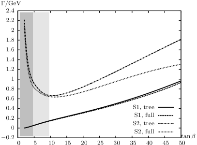
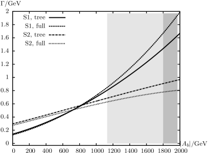
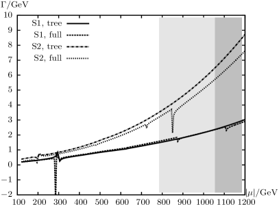
Figure 1: $\Gamma(\tilde{t}_{2}\to\tilde{b}_{1}H^{+})$. Tree-level and full one-loop corrected partial decay widths for the renormalization scheme RS2. The parameters are chosen according to the scenarios S1 and S2. For S1 the grey region is excluded and for S2 the dark grey region is excluded. Upper left plot: $\tan\beta$ varied. Upper right plot: $\tan\beta=20$ and $|A_{b}|$ varied. Lower left plot: $\tan\beta=20$ and $|\mu|$ varied. Lower right plot: $\tan\beta=20$ and $\varphi_{A_{b}}$ varied.

In Fig. 1 we show the partial decay width $\Gamma(\tilde{t}_{2}\to\tilde{b}_{1}H^{+})$ as a function of $\tan\beta$ (upper left), as a function of $A_{b}$ (upper right), as a function of $\mu$ (lower left) and as a function of $\varphi_{A_{b}}$ (lower right plot). “tree” denotes the tree-level value and “full” is the decay width including all one-loop corrections (including hard QED and QCD radiation, see Ref. [3] for details). For S1 the grey region is excluded and for S2 the dark grey region is excluded. The spikes and dips visible in the lower left plot are due to various particle thresholds, while the first dip in S1 is due to $|U_{\tilde{b}_{11}}|\approx|U_{\tilde{b}_{12}}|$. The two spikes in the lower right plot are also due to $|U_{\tilde{b}_{11}}|\approx|U_{\tilde{b}_{12}}|$, which leads to a divergence in RS2, which, however, is confined to very narrow intervals. The loop corrections, as can be observed in all four plots, are relatively modest, staying below $\sim 25\%$ for all parameters. The fact of relatively small one-loop corrections shows that no unphysically large contributions via large counterterms are introduced, a characteristic of a suitable renormalization scheme.

The real quantity of interest at the LHC is the ${\rm BR}(\tilde{t}_{2}\to\tilde{b}_{1}H^{+})$. This, however, requires the evaluation of all decay modes (at the same level of accuracy). The corresponding results will be presented elsewhere [12].

Acknowledgements

S.H. thanks the organizers of cHarged 2010 for the invitation and an inspiring workshop. Work supported in part by the European Community’s Marie-Curie Research Training Network under contract MRTN-CT-2006-035505 ‘Tools and Precision Calculations for Physics Discoveries at Colliders’.

References

• [1]
• [2] H.P. Nilles, Phys. Rept. 110 (1984) 1;
H.E. Haber and G.L. Kane, Phys. Rept. 117 (1985) 75;
R. Barbieri, Riv. Nuovo Cim. 11 (1988) 1.
• [3] S. Heinemeyer, H. Rzehak and C. Schappacher, Phys. Rev. D 82 (2010) 075010 [arXiv:1007.0689 [hep-ph]].
• [4] S. Heinemeyer, W. Hollik and G. Weiglein, Comput. Phys. Commun. 124 (2000) 76 [arXiv:hep-ph/9812320]; see www.feynhiggs.de .
• [5] S. Heinemeyer, W. Hollik and G. Weiglein, Eur. Phys. J. C 9 (1999) 343 [arXiv:hep-ph/9812472].
• [6] G. Degrassi, S. Heinemeyer, W. Hollik, P. Slavich and G. Weiglein, Eur. Phys. J. C 28 (2003) 133 [arXiv:hep-ph/0212020].
• [7] M. Frank, T. Hahn, S. Heinemeyer, W. Hollik, R. Rzehak and G. Weiglein, JHEP 0702 (2007) 047 [arXiv:hep-ph/0611326].
• [8] S. Heinemeyer, W. Hollik, H. Rzehak and G. Weiglein, Phys. Lett. B 652 (2007) 300 [arXiv:0705.0746 [hep-ph]].
• [9] H. Rzehak, PhD thesis: “Two-loop contributions in the supersymmetric Higgs sector”, Technische Universität München, 2005; see: nbn-resolving.de/
with urn: nbn:de:bvb:91-diss20050923-0853568146 .
• [10] J. Küblbeck, M. Böhm and A. Denner, Comput. Phys. Commun. 60 (1990) 165;
T. Hahn, Comput. Phys. Commun. 140 (2001) 418 [arXiv:hep-ph/0012260];
T. Hahn and C. Schappacher, Comput. Phys. Commun. 143 (2002) 54 [arXiv:hep-ph/0105349].
The program and the user’s guide are available via www.feynarts.de .
• [11] A. Fowler and G. Weiglein, JHEP 1001 (2010) 108 [arXiv:0909.5165 [hep-ph]].
• [12] T. Fritzsche, S. Heinemeyer, H. Rzehak, C. Schappacher and G. Weiglein, in preparation.