The Development of Dominance Stripes and Orientation Maps in a Self-Organising Visual Cortex Network (VICON)

A self-organising neural network is presented that is based on a rigorous Bayesian analysis of the information contained in individual neural firing events. This leads to a visual cortex network (VICON) that has many of the properties emerge when a mammalian visual cortex is exposed to data arriving from two imaging sensors (i.e. the two retinae), such as dominance stripes and orientation maps.

1 Introduction

The overall goal of this work is to automate as far as is possible the processing of data from multiple sensors (data fusion), which includes the automatic design of the architecture and functionality of the network(s) that do the processing. In [11] a novel approach to this automation problem was introduced, and the purpose of this paper is to refine and extend the previously reported results.

The problem of automating the design of a data fusion network has many interesting special case solutions. In particular, the type of self-organising neural network (in the mammalian visual cortex) that processes the images arriving from a pair of retinae is one such special case, where the number of sensors involved is just two. For a review of visual cortex neural network models see [2, 14].

The basic idea is to use a soft encoder (i.e. its output is a distributed code in which more than one, and possibly all, of the output neurons is active) to transform the input vector (i.e. the input image) into a posterior probability over various possible classes (i.e. alternative possible interpretations of the input vector), and to optimise the encoder so that this posterior probability is able to retain as much information as possible about the input vector, as measured in the minimum mean square reconstruction error (i.e. $L_{2}$ error) sense [9, 10].

In the special case where the optimisation is performed over the space of all possible soft encoders, the optimum solution is a hard encoder (i.e. it is a “winner-take-all” network in which only one of the output neurons is active) which is an optimal vector quantiser (VQ), of the type described in [4], for encoding the input vector with minimum $L_{2}$ error. In the slightly less special case where the space of possible soft encoders is restricted to include only those whose output is deliberately damaged by the effects of a noise process, this produces a different type of hard encoder which is an optimal self-organising map (SOM) for encoding the input vector with minimum $L_{2}$ error; this is very closely related to the well-known Kohonen map [3], as was demonstrated in [5].

This paper will examine yet another special case, where the optimisation is performed over a very special subspace of soft encoders, rather than over all possible soft encoders. The behaviour of each soft encoder is modelled by a set of posterior probabilities over various possible classes. When a particular parametric form for these posterior probabilities is chosen, a corresponding subspace of possible soft encoders is thus automatically selected, which may be explored by varying the parameters. The parametric form of the posterior probability that is used in this paper is based on the so-called partitioned mixture distribution (PMD) [7, 8], which is a natural generalisation of the standard mixture distribution to a high-dimensional input space.

This use of a PMD leads to a 2-layer visual cortex network (VICON), where the components of the input vector are the output activities of the input neurons, and the components of the PMD posterior probability are the output activities of the output neurons. Various physically realistic constraints are placed on the PMD optimisation (both on the internal PMD structure, and on the type of training data that is used), and these will be described in the text as they arise.

The layout of this paper is as follows. In section 2 all of the necessary theoretical machinery is developed, including folded Markov chains, posterior probability models, derivatives of the objective function, and receptive fields. In section 3 the concepts of dominance stripes and orientation maps are explained, both in the context of the elastic net model, and in the context of theory presented in this paper. In section 4 the results of computer simulations are presented, including both 1 and 2-dimensional retinae, single and pairs of retinae, both for synthetic and natural training data. In appendix B some explicit optimal solutions that minimise the objective function are derived, including the periodicity property of some types of optimal solution.

2 Theory

This section covers all of the basic theoretical machinery that is required to design and train a 2-layer VICON. In section 2.1 the theory of folded Markov chains (FMC) is summarised. In section 2.2 the basic idea of a posterior probability model is introduced, and in section 2.3 this is developed into a full partitioned posterior probability model. In section 2.4 the derivatives of the FMC objective function are derived assuming a partitioned posterior probability model, and in section 2.5 the influence of finite-sized receptive fields on these derivatives is derived.

2.1 Folded Markov Chain

The basis of the entire theoretical treatment is a communication channel model [6] in which an input vector $\mathbf{x}$ is encoded to produce a conditional probability $\Pr\left(y|\mathbf{x}\right)$ over code indices $y$, which is then transmitted along a distorting communication channel to produce a conditional probability $\Pr\left(y^{\prime}|y\right)$ over distorted code indices $y^{\prime}$, which is finally decoded to produce a conditional PDF $\Pr\left(\mathbf{x}^{\prime}|y^{\prime}\right)$ over reconstructions $\mathbf{x}^{\prime}$ of the original input vector $\mathbf{x}$. The three steps in the sequence $\mathbf{x\rightarrow}y\mathbf{\rightarrow}y^{\prime}\mathbf{\rightarrow x}^{\prime}$ are modelled by the conditional probabilities $\Pr\left(y|\mathbf{x}\right)$, $\Pr\left(y^{\prime}|y\right)$, and $\Pr\left(\mathbf{x}^{\prime}|y^{\prime}\right)$, which describe a Markov chain of transitions, which is shown diagrammatically in figure 1(a). $\Pr\left(\mathbf{x}^{\prime}|y\right)$ is completely determined from other defined quantities by using Bayes’ theorem in the form $\Pr\left(\mathbf{x}|y\right)=\frac{\Pr\left(\mathbf{x}\right)\Pr\left(y|\mathbf{x}\right)}{\int d\mathbf{x}^{\prime}\Pr\left(\mathbf{x}^{\prime}\right)\Pr\left(y|\mathbf{x}^{\prime}\right)}$.

Because $\mathbf{x}$ and $\mathbf{x}^{\prime}$ live in the same vector space it is convenient to fold this diagram to produce figure 1(b); this is called a folded Markov chain (FMC) [6].

Figure 1: (a) A Markov chain of transitions $\mathbf{x\rightarrow}y\mathbf{\rightarrow}y^{\prime}\mathbf{\rightarrow x}^{\prime}$. (b) The same diagram as (a), but folded.

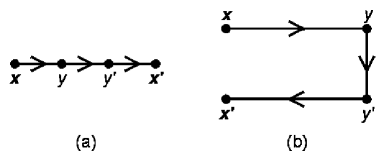
Figure 1(b) is directly related to a 2-layer unsupervised neural network, where $\mathbf{x}$ and $\mathbf{x}^{\prime}$ represent the activity pattern of the whole set of neurons in the input layer, and $y$ and $y^{\prime}$ represent the location(s) of winning neuron(s) in the ouput layer. The overall conditional PDF generated by an FMC is $\Pr(\mathbf{x}^{\prime}|\mathbf{x})$, which is obtained by marginalising $y$ and $y^{\prime}$ in the joint probability $\Pr\left(\mathbf{x}^{\prime},y^{\prime},y|\mathbf{x}\right)=\Pr\left(\mathbf{x}^{\prime}|y^{\prime}\right)\Pr\left(y^{\prime}|y\right)\Pr\left(y|\mathbf{x}\right)$.

Define a network objective function $D$ as [6]

$$D=\int d\mathbf{x}\,d\mathbf{x}^{\prime}\Pr\left(\mathbf{x}\right)\Pr(\mathbf{x}^{\prime}|\mathbf{x})\,\left\|\mathbf{x}-\mathbf{x}^{\prime}\right\|^{2}$$ (1)

which measures the expected Euclidean (or $L_{2}$) reconstruction error caused by feeding input vectors sampled from $\Pr\left(\mathbf{x}\right)$ into the FMC, where each $\mathbf{x}$ is returned as a PDF $\Pr(\mathbf{x}^{\prime}|\mathbf{x})$ of alternative reconstructions $\mathbf{x}^{\prime}$ of $\mathbf{x}$. For simplicity, assume that the communication channel has been assumed to be distortionless so that $\Pr\left(y^{\prime}|y\right)=\delta_{yy^{\prime}}$, and that $y=1,2,\cdots,M$, then

$$D=\sum_{y=1}^{M}\int d\mathbf{x}\,d\mathbf{x}^{\prime}\Pr\left(\mathbf{x}\right)\Pr\left(y|\mathbf{x}\right)\Pr\left(\mathbf{x}^{\prime}|y\right)\,\left\|\mathbf{x}-\mathbf{x}^{\prime}\right\|^{2}$$ (2)

An FMC is completely described by the form of its encoder $\Pr\left(y|\mathbf{x}\right)$ and the form of its reconstruction error $\left\|\mathbf{x}-\mathbf{x}^{\prime}\right\|^{2}$. The functional form of the encoder may be chosen arbitrarily, and independently of the assumed Euclidean form of the reconstruction error, so the FMC does not correspond to a Gaussian mixture distribution model in input space. This is a general result for FMCs in which the functional forms of the encoder and the reconstruction error may be independently chosen. It is only when these functional forms are carefully chosen that a density model interpretation of an FMC is possible (for instance a Euclidean reconstruction error $\left\|\mathbf{x}-\mathbf{x}^{\prime}\right\|^{2}$ must be paired with an encoder $\Pr\left(y|\mathbf{x}\right)$ that describes the posterior probability over class labels that would arise in a Gaussian mixture distribution model).

The expression for $D$ given in equation 2 may be simplified to yield [6] (this readily generalises to the case where $\Pr\left(y^{\prime}|y\right)\neq\delta_{yy^{\prime}}$ (i.e. the communication channel causes distortion))

$$D=2\int d\mathbf{x}\Pr\left(\mathbf{x}\right)\sum_{y=1}^{M}\Pr\left(y|\mathbf{x}\right)\left\|\mathbf{x}-\mathbf{x}^{\prime}\left(y\right)\right\|^{2}$$ (3)

where $\mathbf{x}^{\prime}\left(y\right)$ is a reference vector defined as

$$\mathbf{x}^{\prime}\left(y\right)\equiv\int d\mathbf{x}\Pr\left(\mathbf{x}|y\right)\mathbf{x}$$ (4)

If this definition of $\mathbf{x}^{\prime}\left(y\right)$ is not used, and instead $D$ in equation 3 is minimised with respect to $\mathbf{x}^{\prime}\left(y\right)$, then the stationary solution is $\mathbf{x}^{\prime}\left(y\right)=\int d\mathbf{x}\Pr\left(\mathbf{x}|y\right)\mathbf{x}$, which is consistent with the definition in equation 4. In practice, it is better to determine the stationary $\mathbf{x}^{\prime}\left(y\right)$ by following the gradient $\frac{\partial D}{\partial\mathbf{x}^{\prime}\left(y\right)}$ than to use the explicit expression $\int d\mathbf{x}\Pr\left(\mathbf{x}|y\right)\mathbf{x}$ for the stationary point, because $\frac{\partial D}{\partial\mathbf{x}^{\prime}\left(y\right)}$ is cheap to evaluate whereas $\int d\mathbf{x}\Pr\left(\mathbf{x}|y\right)\mathbf{x}$ is expensive to evaluate. In effect, the $\frac{\partial D}{\partial\mathbf{x}^{\prime}\left(y\right)}$ approach is an example of on-line training, whereas the $\int d\mathbf{x}\Pr\left(\mathbf{x}|y\right)\mathbf{x}$ approach is the corresponding example of batch training, and the on-line and batch approaches each have their own areas where they are best used.

In equation 3 $\Pr\left(y|\mathbf{x}\right)$ is a “recognition model” (i.e. it takes an input vector and recognises by assigning to it a posterior probability over class labels) and $\mathbf{x}^{\prime}\left(y\right)$ is the corresponding “generative model” (i.e. it takes a class label and generates a corresponding vector in input space). This is a simpler type of generative model than appeared in the original expression for $D$ in equation 2, where the generative model is $\Pr\left(\mathbf{x}^{\prime}|y\right)$, which generates a whole distribution of possible vectors in input space, rather than just a single vector which is the centroid of $\Pr\left(\mathbf{x}^{\prime}|y\right)$. The transformation of the FMC from one that uses the PDF $\Pr\left(\mathbf{x}^{\prime}|y\right)$ into one that uses the reference vector $\mathbf{x}^{\prime}\left(y\right)$ is not possible in general; it was made possible here by choosing to use a Euclidean reconstruction error in $D$. In general, an FMC reconstruction is a distribution over alternative inputs, rather than a single representative input, as might be used in decision theory, for instance.

The operation of the various terms in the expression for $D$ in equation 3 is shown in figure 2, which is rotated through 90^∘ anticlockwise with respect to the corresponding diagram in figure 1, and also for simplicity $y^{\prime}=y$ because $\Pr\left(y^{\prime}|y\right)=\delta_{yy^{\prime}}$ was assumed above.

Figure 2: A neural network representation of a folded Markov chain.

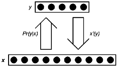
When $D$ is minimised with respect to the choice of encoder $\Pr\left(y|\mathbf{x}\right)$ and reconstruction vector $\mathbf{x}^{\prime}\left(y\right)$ it yields a standard minimum mean square error vector quantiser (VQ) with $M$ code indices [4], and if $\Pr\left(y^{\prime}|y\right)\neq\delta_{yy^{\prime}}$ then the VQ produces code indices that carry information in such a way that it is maximally robust with respect to the damaging effects of communication channel distortion modelled by $\Pr\left(y^{\prime}|y\right)$ [5]. This latter type of VQ can be shown to be approximately equivalent to a self-organising map (SOM) of the type introduced by Kohonen [3].

2.2 Basic Posterior Probability (Single Recognition Model)

The minimisation procedure that leads to a VQ-like optimum assumed that the entire space of posterior probability functions $\Pr\left(y|\mathbf{x}\right)$ was available to be searched. In the neural network interpretation, $\Pr\left(y|\mathbf{x}\right)$ models the probability that neuron $y$ fires first (this encompasses both the case of a soft encoder where more than one neuron can potentially fire first, and the case of a hard encoder where only one neuron can potentially fire first; this is the winner-take-all case), which depends on the detailed underlying dynamics of how all of the neurons interact with each other. Because these neural dynamics are not arbitrary (e.g. they are constrained to be a physically realisable process), it constrains the space of possible posterior probabilities $\Pr\left(y|\mathbf{x}\right)$ that is available to the neural network. $\Pr\left(y|\mathbf{x}\right)$ may then be modelled by the functional form

$$\Pr\left(y|\mathbf{x}\right)\equiv\frac{Q\left(\mathbf{x|}y\right)}{\sum_{y^{\prime}=1}^{M}Q\left(\mathbf{x|}y^{\prime}\right)}$$ (5)

where $Q\left(\mathbf{x|}y\right)$ is the raw “response function” of neuron $y$.

$Q\left(\mathbf{x|}y\right)$ may be interpreted as the raw firing rate of neuron $y$, and $\Pr\left(y|\mathbf{x}\right)$ is then the probability that neuron $y$ fires first out of all of the $M$ competing neurons. This functional form makes it clear that there is a type of lateral inhibition occurring between $\Pr\left(y_{1}|\mathbf{x}\right)$ and $\Pr\left(y_{2}|\mathbf{x}\right)$ (for $y_{1}\neq y_{2}$), because if the raw firing rate $Q\left(\mathbf{x|}y_{1}\right)$ is increased so that $\Pr\left(y_{1}|\mathbf{x}\right)$ increases, nevertheless the denominator $\sum_{y^{\prime}=1}^{M}Q\left(\mathbf{x|}y^{\prime}\right)$ ensures that $\Pr\left(y_{2}|\mathbf{x}\right)$ decreases (for $y_{1}\neq y_{2}$); i.e. the $Q\left(\mathbf{x|}y\right)$ do not exhibit lateral inhibition, but the $\Pr\left(y_{1}|\mathbf{x}\right)$ do exhibit lateral inhibition.

The raw receptive field of a neuron depends on the form of $Q\left(\mathbf{x|}y\right)$. Thus if the functional form of $Q\left(\mathbf{x|}y\right)$ depends only on a subset $\mathbf{\tilde{x}}\left(y\right)$ of components of $\mathbf{x}$, then $\mathbf{\tilde{x}}\left(y\right)$ is the raw receptive field of neuron $y$. However, this is not the same as the the receptive field that is effective in producing the first firing event, because $\Pr\left(y|\mathbf{x}\right)$ depends on all of the $\mathbf{\tilde{x}}\left(y^{\prime}\right)$ (for $y^{\prime}=1,\cdots,M$) as shown in equation 5.

The effect of the distortion $\Pr\left(y\mathbf{|}y\mathbf{{}^{\prime}}\right)$ process, as modelled by $\Pr\left(y\mathbf{|}y\mathbf{{}^{\prime}}\right)$, is to alter at the last minute, as it were, the probability that each neuron fires first. Thus the posterior probability is modified as follows

$$\Pr\left(y|\mathbf{x}\right)\rightarrow\sum_{y^{\prime}=1}^{M}\Pr\left(y\mathbf{|}y\mathbf{{}^{\prime}}\right)\Pr\left(y^{\prime}|\mathbf{x}\right)$$ (6)

where the matrix element $\Pr\left(y\mathbf{|}y\mathbf{{}^{\prime}}\right)$ leaks posterior probability from neuron $y^{\prime}$ onto neuron $y$. Such cross-talk amongst the neurons exists independently of the lateral inhibition effect produced by the denominator term $\sum_{y^{\prime}=1}^{M}Q\left(\mathbf{x|}y^{\prime}\right)$ in equation 5.

The VQ and SOM results (see [4, 3]) may be obtained as special cases of raw neuron firing rates $Q\left(\mathbf{x|}y\right)$, where one neuron’s firing rate is much larger than the other $M-1$ neurons’ firing rates (i.e. there is effectively only one neuron that can fire, so it is the winner-take-all).

2.3 Partitioned Posterior Probability (Multiple Recognition Models)

The form of the posterior probability $\Pr\left(y|\mathbf{x}\right)$ introduced in equation 5 is unsuitable for networks with a large number of neurons $M$, because the lateral inhibition is global rather than local. This can readily be inferred because the denominator term $\sum_{y^{\prime}=1}^{M}Q\left(\mathbf{x|}y^{\prime}\right)$ in equation 5 computes a quantity that is the sum over all of the raw neuron firing rates.

This problem can be amended by defining a localised posterior probability $\Pr\left(y|\mathbf{x;}y^{\prime}\right)$ as

$$\Pr\left(y|\mathbf{x;}y^{\prime}\right)\equiv\frac{Q\left(\mathbf{x|}y\right)\delta_{y\in\mathcal{N}\left(y^{\prime}\right)}}{\sum_{y^{\prime\prime}\in\mathcal{N}\left(y^{\prime}\right)}Q\left(\mathbf{x|}y^{\prime\prime}\right)}$$ (7)

where $\mathcal{N}\left(y^{\prime}\right)$ is the local neighbourhood of neuron $y^{\prime}$, which is assumed to contain at least neuron $y^{\prime}$, and $\delta_{y\in\mathcal{N}\left(y^{\prime}\right)}$ is a Kronecker delta that constrains $y$ to lie in the neighbourhood $\mathcal{N}\left(y^{\prime}\right)$. If $\mathcal{N}\left(y^{\prime}\right)$ contains all $M$ neurons then $\Pr\left(y|\mathbf{x;}y^{\prime}\right)$ reduces to $\Pr\left(y|\mathbf{x}\right)$ as previously defined in equation 5. $\Pr\left(y|\mathbf{x;}y^{\prime}\right)$ has the required normalisation property that $\sum_{y=1}^{M}\Pr\left(y|\mathbf{x;}y^{\prime}\right)=1$ for all $y^{\prime}$. Because $y^{\prime}$ can take $M$ possible values, there are $M$ complete localised posterior probability functions $\Pr\left(y|\mathbf{x;}y^{\prime}\right)$. In effect, the neural network is split up into $M$ overlapping subnetworks (these subnetworks overlap where $\mathcal{N}\left(y_{1}\right)\cap\mathcal{N}\left(y_{2}\right)\neq\emptyset$ for $y_{1}\neq y_{2}$), each of which computes its own posterior probability function; note that any overlap between a pair of subnetworks causes the corresponding $\Pr\left(y|\mathbf{x;}y^{\prime}\right)$ to be mutually dependent.

It is not always convenient to use a neural network model in which there are $M$ separate posterior probability models $\Pr\left(y|\mathbf{x;}y^{\prime}\right)$. However, these $M$ localised posterior probability functions $\Pr\left(y|\mathbf{x;}y^{\prime}\right)$ (for the $M$ different choices of $y^{\prime}$) may be averaged together to produce a single posterior probability function. Thus define $\Pr\left(y|\mathbf{x}\right)$ as

$$\Pr\left(y|\mathbf{x}\right) \equiv \frac{1}{M}\sum_{y^{\prime}\in\mathcal{N}^{-1}\left(y\right)}\Pr\left(y|\mathbf{x;}y^{\prime}\right)$$ (8)

$$= \frac{1}{M}\,Q\left(\mathbf{x|}y\right)\sum_{y^{\prime}\in\mathcal{N}^{-1}\left(y\right)}\frac{1}{\sum_{y^{\prime\prime}\in\mathcal{N}\left(y^{\prime}\right)}Q\left(\mathbf{x|}y^{\prime\prime}\right)}$$

where $\mathcal{N}^{-1}\left(y\right)$ is the inverse neighbourhood of neuron $y$ defined as $\mathcal{N}^{-1}\left(y\right)\equiv\left\{y^{\prime}|y\in\mathcal{N}\left(y^{\prime}\right)\right\}$. This definition has all of the properties of a posterior probability function, including the normalisation property $\sum_{y=1}^{M}\Pr\left(y|\mathbf{x}\right)=1$ (which may be derived by swapping the order of summations using the result $\sum_{y=1}^{M}\sum_{y^{\prime}\in\mathcal{N}^{-1}\left(y\right)}\left(\cdots\right)=\sum_{y^{\prime}=1}^{M}\sum_{y\in\mathcal{N}\left(y^{\prime}\right)}\left(\cdots\right)$). The form of the posterior probability given in equation 8, in which $M$ individual posterior probabilities $\Pr\left(y|\mathbf{x;}y^{\prime}\right)$ are averaged together, can be rigorously justified from a Bayesian point of view (see appendix A). The averaging process produces the posterior probability that should be used when there are $M$ contributing models (as specified by the $\Pr\left(y|\mathbf{x;}y^{\prime}\right)$ for $y^{\prime}=1,2,\cdots,M$) that have equal prior weight. The average over the $M$ models then simply marginalises over an unobserved degree of freedom (the model index $y^{\prime}$).

If this localised definition of $\Pr\left(y|\mathbf{x}\right)$ given in equation 8 is compared with the global definition given in equation 5 it is seen that the normalisation factor has been modified thus

$$\frac{1}{\sum_{y^{\prime}=1}^{M}Q\left(\mathbf{x|}y^{\prime}\right)}\rightarrow\frac{1}{M}\sum_{y^{\prime}\in\mathcal{N}^{-1}\left(y\right)}\frac{1}{\sum_{y^{\prime\prime}\in\mathcal{N}\left(y^{\prime}\right)}Q\left(\mathbf{x|}y^{\prime\prime}\right)}$$ (9)

which alters its lateral inhibition properties. $\frac{1}{\sum_{y^{\prime\prime}\in\mathcal{N}\left(y^{\prime}\right)}Q\left(\mathbf{x|}y^{\prime\prime}\right)}$ is the lateral inhibition factor that derives from the neighbourhood of neuron $y^{\prime}$, which gives rise to a contribution to the lateral inhibition factor for all neurons $y$ in the neighbourhood of $y^{\prime}$ via the average $\frac{1}{M}\sum_{y^{\prime}\in\mathcal{N}^{-1}\left(y\right)}\left(\cdots\right)$. Thus the overall lateral inhibition factor acting on neuron $y$ is derived locally from those neurons $y^{\prime\prime}$ that lie in the set $\mathcal{N}\left(\mathcal{N}^{-1}\left(y\right)\right)$. The posterior probability model defined in equation 8 has been used before in the context of partitioned mixture distributions (PMDs), where multiple mixture distribution models are simultaneously optimised [7, 8].

Figure 3 shows the structure of the neural network corresponding to the PMD posterior probability in equation 8.

Figure 3: A partitioned mixture distribution (PMD) neural network.

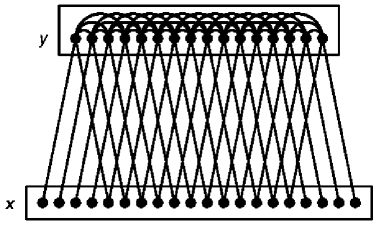
Each output neuron has a raw receptive field of input neurons (which contains 5 input neurons in the example shown), and is also laterally inhibited by its neighbouring output neurons (the size of a neuron neighbourhood is 3 neurons to either side in the example shown). Note that the input-output links in figure 3 do not imply that the raw neuron firing rates $Q\left(\mathbf{x|}y\right)$ can be computed by using simple weighted connections; they are drawn merely to indicate the set of input neurons that influences the raw firing rate of each output neuron. Similarly, the output-output links in figure 3 are drawn to indicate the sizes of the output neuron neighbourhoods; the details of how lateral inhibition modifies the raw firing rates $Q\left(\mathbf{x|}y\right)$ of the output neurons to produce the probability $\Pr\left(y|\mathbf{x}\right)$ that neuron $y$ fires first is given in equation 8.

For completeness, the PMD objective function in equation 3 may now be written out in full using the expression for the PMD posterior probability in equation 8 to yield (where the effects of leakage have been included, as defined in equation 6)

$$D = \frac{2}{M}\int d\mathbf{x}\Pr\left(\mathbf{x}\right)\sum_{y=1}^{M}\sum_{y^{\prime}=1}^{M}\Pr\left(y\mathbf{|}y\mathbf{{}^{\prime}}\right)$$ (10)

$$\times\,Q\left(\mathbf{x|}y^{\prime}\right)\sum_{y^{\prime\prime}\in\mathcal{N}^{-1}\left(y^{\prime}\right)}\frac{1}{\sum_{y^{\prime\prime\prime}\in\mathcal{N}\left(y^{\prime\prime}\right)}Q\left(\mathbf{x|}y^{\prime\prime\prime}\right)}\left\|\mathbf{x}-\mathbf{x}^{\prime}\left(y\right)\right\|^{2}$$

This is the objective function that will be used to characterise to performance of the neural networks in all of the computer simulations.

2.4 Derivatives of the Objective Function

In order to minimise the PMD objective function in equation 10 its derivatives must be calculated. First of all, define some convenient notation [10]

$$\begin{array}[]{ll}L_{y,y^{\prime}}\equiv\Pr\left(y\mathbf{{}^{\prime}|}y\right)&P_{y,y^{\prime}}\equiv\Pr\left(y\mathbf{{}^{\prime}|x;}y\right)\equiv\frac{Q\left(\mathbf{x|}y^{\prime}\right)\delta_{y^{\prime}\in\mathcal{N}\left(y\right)}}{\sum_{y^{\prime\prime}\in\mathcal{N}\left(y\right)}Q\left(\mathbf{x|}y^{\prime\prime}\right)}\\ p_{y}\equiv\sum_{y^{\prime}\in\mathcal{N}^{-1}\left(y\right)}P_{y^{\prime},y}&\left(L^{T}p\right)_{y}\equiv\sum_{y^{\prime}\in\mathcal{L}^{-1}\left(y\right)}L_{y^{\prime}\mathbf{,}y}p_{y^{\prime}}\\ e_{y}\equiv\left\|\mathbf{x}-\mathbf{x}^{\prime}\left(y\right)\right\|^{2}&\left(Le\right)_{y}\equiv\sum_{y^{\prime}\in\mathcal{L}\left(y\right)}L_{y,y^{\prime}}e_{y^{\prime}}\\ \left(PLe\right)_{y}\equiv\sum_{y^{\prime}\in\mathcal{N}\left(y\right)}P_{y,y^{\prime}}\left(Le\right)_{y^{\prime}}&\left(P^{T}PLe\right)_{y}\equiv\sum_{y^{\prime}\in\mathcal{N}^{-1}\left(y\right)}P_{y\mathbf{{}^{\prime},}y}\left(PLe\right)_{y^{\prime}}\end{array}$$ (11)

where $\mathcal{L}\left(y\right)$ denotes the leakage neighbourhood of neuron $y$, which is the set of neurons that have posterior probability leaked onto them by neuron $y$, and the inverse leakage neighbourhood $\mathcal{L}^{-1}\left(y\right)$ is defined as $\mathcal{L}^{-1}\left(y\right)\equiv\left\{y^{\prime}|y\in\mathcal{L}\left(y^{\prime}\right)\right\}$. Assume that the raw neuron firing rates may be modelled using a sigmoid function

$$Q\left(\mathbf{x}|y\right)=\frac{1}{1+\exp\left(-\mathbf{w}\left(y\right)\cdot\mathbf{x}-b\left(y\right)\right)}$$ (12)

whence the derivatives may be obtained in the form [10]

$$\frac{\partial D}{\partial\mathbf{x}^{\prime}\left(y\right)} = -\frac{4}{M}\int d\mathbf{x}\Pr\left(\mathbf{x}\right)\left(L^{T}p\right)_{y}\left(\mathbf{x}-\mathbf{x}^{\prime}\left(y\right)\right)$$

$$\frac{\partial D}{\partial\left(\begin{array}[]{l}b\left(y\right)\\ \mathbf{w}\left(y\right)\end{array}\right)} = \frac{2}{M}\int d\mathbf{x}\Pr\left(\mathbf{x}\right)\left[\begin{array}[]{c}\left(p_{y}\left(Le\right)_{y}-(P^{T}PLe)_{y}\right)\\ \times\left(1-Q\left(\mathbf{x}|y\right)\right)\left(\begin{array}[]{l}1\\ \mathbf{x}\end{array}\right)\end{array}\right]$$ (19)

where the two derivatives $\frac{\partial D}{\partial b\left(y\right)}$ and $\frac{\partial D}{\partial\mathbf{w}\left(y\right)}$ have been written together for compactness.

2.5 Receptive Fields

The raw firing rate $Q\left(\mathbf{x}|y\right)$ of neuron $y$ depends only on a subset $\mathbf{\tilde{x}}\left(y\right)$ of components of $\mathbf{x}$; $\mathbf{\tilde{x}}\left(y\right)$ is thus the raw receptive field of neuron $y$. However, the posterior probability $\Pr\left(y|\mathbf{x}\right)$ that neuron $y$ fires first is derived from $Q\left(\mathbf{x}|y\right)$ by weighting it with a lateral inhibition factor that depends on the raw firing rates of all neurons in $\mathcal{N}\left(\mathcal{N}^{-1}\left(y\right)\right)$, as seen in equation 8, so the overall receptive field of a neuron is rather broader than its raw receptive field. The effect of leakage, as defined in equation 6, is to broaden the overall receptive field further still. The optimal reference vector $\mathbf{x}^{\prime}\left(y\right)$ has non-trivial structure only within this overall receptive field, so inside the overall receptive field the components of $\mathbf{x}^{\prime}\left(y\right)$ must be subjected to an optimisation procedure to discover their optimal form, whereas outside the overall receptive field the components of $\mathbf{x}^{\prime}\left(y\right)$ may be set to be the average values of the corresponding components of the training vectors $\mathbf{x}$ (see the definition of $\mathbf{x}^{\prime}\left(y\right)$ in equation 4, which reduces to $\mathbf{x}^{\prime}\left(y\right)=\int d\mathbf{x}\Pr\left(\mathbf{x}\right)\mathbf{x}$ for those components of $\mathbf{x}^{\prime}\left(y\right)$ that lie outside the overall receptive field of neuron $y$).

In the simulations that will be presented here a suboptimal approach is used, where only those components of $\mathbf{x}^{\prime}\left(y\right)$ that lie inside the raw receptive field are optimised; this produces a least upper bound on the value of the objective function that would have been obtained if a full optimisation had been used. Also, it is assumed that the input data has been prepared in such a way that each component is zero mean. This is not actually a restriction, because the objective function is invariant with respect to adding a different constant to each component of $\mathbf{x}$, because it is a function of the difference $\mathbf{x}-\mathbf{x}^{\prime}$. In this suboptimal approach, and with the zero mean assumption, the components of $\mathbf{x}^{\prime}\left(y\right)$ that lie outside the raw receptive field of neuron $y$ will be set to zero.

The fact that the components of $\mathbf{x}^{\prime}\left(y\right)$ that lie outside the raw receptive field of neuron $y$ are zero may be used to simplify the evaluation of the various terms $\frac{\partial D}{\partial b\left(y\right)}$ and $\frac{\partial D}{\partial\mathbf{w}\left(y\right)}$ in equation 19. Thus evaluate $p_{y}\left(Le\right)_{y}-(P^{T}PLe)_{y}$ by expanding $e_{y}$ as

$$e_{y} = \left\|\mathbf{x}\right\|^{2}-2\mathbf{x}\cdot\mathbf{x}^{\prime}\left(y\right)+\left\|\mathbf{x}^{\prime}\left(y\right)\right\|^{2}$$ (20)

$$= \left\|\mathbf{x}\right\|^{2}+\mathbf{x}^{\prime}\left(y\right)\cdot\left(\mathbf{x}^{\prime}\left(y\right)-2\mathbf{x}\right)$$

which is a sum of a constant (i.e. does not depend on $y$) term $\left\|\mathbf{x}\right\|^{2}$ and a term $\mathbf{x}^{\prime}\left(y\right)\cdot\left(\mathbf{x}^{\prime}\left(y\right)-2\mathbf{x}\right)$ that does depend on $y$. What happens to the constant term when it is substituted into $p_{y}\left(Le\right)_{y}-(P^{T}PLe)_{y}$?

$$p_{y}\left(Le\right)_{y}-(P^{T}PLe)_{y} \rightarrow p_{y}\left(L\cdot\mathbf{1}\right)_{y}-(P^{T}PL\cdot\mathbf{1})_{y}$$ (21)

$$= p_{y}\mathbf{1}_{y}-(P^{T}P\cdot\mathbf{1})_{y}$$

$$= p_{y}-p_{y}$$

$$= 0$$

It cancels out, so $e_{y}$ might as well be replaced as follows in $p_{y}\left(Le\right)_{y}-(P^{T}PLe)_{y}$

$$e_{y}\rightarrow\mathbf{x}^{\prime}\left(y\right)\cdot\left(\mathbf{x}^{\prime}\left(y\right)-2\mathbf{x}\right)$$ (22)

Because the components of $\mathbf{x}^{\prime}\left(y\right)$ that lie outside the raw receptive field of neuron $y$ are set to zero, the $\mathbf{x}^{\prime}\left(y\right)\cdot\left(\cdots\right)$ operation effectively projects out any components of $\left(\cdots\right)$ that happen to lie outside this raw receptive field. This means that the only components of $\mathbf{x}$ in equation 22 that survive are those that lie inside the raw receptive field, so effectively $e_{y}$ depends only on quantities that lie inside the raw receptive field of neuron $y$. Note that a full optimisation of $\mathbf{x}^{\prime}\left(y\right)$, in which all components that lie inside the overall receptive field of neuron $y$ are optimised, would produce a different result.

3 Dominance Stripes and Orientation Maps

The purpose of this section is to discuss the two phenomena of dominance stripes and orientation maps. In section 3.1 a brief review of the popular elastic net model of dominance stripes is presented, and in section 3.2 an informal derivation of the origin of both dominance stripes and orientation maps is given.

3.1 Review of Dominance Stripes Using the Elastic Net Model

The results that will be presented here are, broadly speaking, equivalent to the way in which ocular dominance stripes are obtained in the elastic net model (as reviewed in [2, 14]) as applied to a pair of retinae. The essential features of this type of model of ocular dominance are shown in figure 4 (which is copied from [2]).

Figure 4: An elastic net oscillating back and forth in ocularity between a pair of retinae.

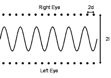
The left and right retinae are represented as 1-dimensional lines of units at the top and bottom of the diagram. The horizontal dimension represents distance across a retina, and the vertical dimension represents the ocularity degree of freedom. The distance between any two retinal units, either within or between retinae, represents the correlation between those two units [2]. Thus the ratio $\frac{l}{d}$ determines the relative strength of the inter-retinal and intra-retinal correlations. The elastic net is represented by the line oscillating back and forth between the retinae. The net effect of the elastic net algorithm is to encourage the elastic net to pass as close as possible (in a well-defined sense) to all of the retinal units, and also to minimise its total length. These are conflicting requirements, and the oscillatory solution shown in figure 4 is typical of an optimal elastic net configuration, which thus predicts an oscillatory pattern of ocular dominance (i.e. which corresponds to dominance stripes in the case of 2-dimensional retinae).

This type of model inevitably leads to dominance stripe formation, because the elastic net model separates the input components into two clusters (see figure 4) according to whether they belong to the left or right retina. In effect the output layer of the network is explicitly told which retina an input component belongs to, and this fact is expressed by the position of the component along the ocularity dimension. The goal in this paper is to construct a more natural model of dominance stripe formation, in which the ocularity dimension is revealed by a process of self-organisation, rather than being hard-wired into the model. Thus, the visual cortex model that is presented in this paper will not explicitly label the input pixels as belonging to the right or left retina (as they are in figure 4), but will have to deduce their left/right retina membership from the properties of the training set instead.

3.2 Informal Derivation of Dominance Stripes and Orientation Maps

The purpose of this section is to present a simple picture that makes it clear what types of behaviour should be expected from neural network that minimises the objective function in equation 10.

3.2.1 Neural Network Model

It is assumed that each of the output neurons has only a limited receptive field of input neurons within each of the two retinae. In effect, this is a hand-crafted version of a “wire length” constraint, which ensures that the total length of the input-to-output connections is limited. In the context of the elastic net model this corresponds to the limited range of interaction between retinal units (the input) and elastic net units (the output). Also, it is assumed that sigmoidal neurons with local probability leakage are used, which generates an effect that is analogous to the elastic tension in the elastic net model, because it encourages neighbouring neurons to adopt similar parameter values.

This model is drawn in figure 5 in an analogous way to the elastic net model in figure 4.

Figure 5: Neural network model with a limited receptive field.

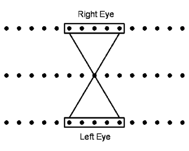
In this model the ocularity dimension is not explicitly present, and the elasticity (of the elastic net) is replaced by the probability leakage mechanism that enables neighbouring output neurons to communicate with each other. The separation of input neurons into left and right retinae in figure 5 is made only for comparison between figure 5 and the elastic net model in figure 4. When the left and right receptive fields are presented to the output neuron, all information about which retina the various input neurons belong to has been discarded; all input neurons within the left and right receptive fields are treated on an equal basis. The ocularity dimension will emerge by a process of self-organisation driven by the statistical properties of the images received by the left and right retinae.

3.2.2 Very Low Resolution Input Images

The simplest situation is when there are two retinae (as in the above elastic net model), each of which senses independently a featureless scene, i.e. all the units in a retina sense the same brightness value, but the two brightnesses that the left and right retinae sense are independent of each other. This situation would arise if the images projected onto the two retinae were very low resolution, so all spatial detail is lost. This limits the input data to lying in a 2-dimensional space $R^{2}$. If these two featureless input images (i.e. left and right retinae) are then normalised so that the sum of left and right retina brightness is constrained to be constant, then the input data is projected down onto a 1-dimensional space $R^{1}$, which effectively becomes the ocularity dimension. If each of the $M$ output neurons had an infinite-sized receptive field, then the optimal network would be the one in which the $M\,$neurons cooperate to give the best soft encoding of $R^{1}$.

However, because of the limited receptive field size and output neuron neighbourhood size, the neurons can at best co-operate together a few at a time (this also depends on the size of the leakage neighbourhood). If the network properties are translation invariant this leads to an optimal network whose properties fluctuate periodically across the network (see appendix B), where each period typically contains a complete repertoire of the computing machinery that is needed to process the contents of a receptive field; this effect is called completeness, and it is a characteristic emergent property of this type of neural network.

The only unexplained step in this argument is the use of a normalisation procedure on the input. However, if the input to this network is the PMD posterior probability computed by the output layer of another such network, then there is already such a normalisation effect induced by the lateral inhibition within the PMD posterior probability. For featureless input images, this lateral inhibition effect causes precisely the type of normalisation that is used above (i.e. left plus right retina brightness is constant) to occur naturally.

These results are summarised in figure 6

Figure 6: Typical neural reference vectors for very low resolution input images.

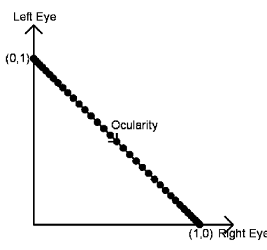
where the ocularity dimension runs from $\left(0,1\right)$ to $\left(1,0\right)$, and a typical set of neural reference vectors is shown. The oscillation of these reference vectors back and forth along the ocularity dimension corresponds to the oscillations of the elastic net that are represented in figure 4.

3.2.3 Low Resolution Input Images

A natural generalisation of the above is to the case of not-quite-featureless input images. This could be brought about by gradually increasing the resolution of the input images until it is sufficient to reveal spatial detail on a size scale equal to the receptive field size. Instead of seeing a featureless input, each neuron would then see a brightness gradient within its receptive field. This could be interpreted by considering the low order terms of a Taylor expansion of the input image about a point at the centre of the neuron’s receptive field: the zeroth term is local average brightness (which lives on a 1-dimensional line $R^{1}$), and the two first order terms are the local brightness gradient (which lives in a 2-dimensional space $R^{2}$). When normalisation is applied this reduces the space in which the two images live to $R^{1}\times R^{2}\times R^{2}$ ($R^{1}$ from the zeroth order Taylor term with normalisation taken into account, $R^{2}$ from the first order Taylor terms, counted twice to deal with each retina).

The $R^{1}$ from the zeroth order Taylor term gives rise to ocular dominance stripes, which thus causes the left and right retinae to map to different stripe-shaped regions of the output layer. The remaining $R^{2}\times R^{2}$ then naturally splits into two contributions (left retina and right retina), each of which maps to the appropriate stripe. If the stripes did not separate the left and right retinae, then the $R^{2}\times R^{2}$ could not be split apart in this simple manner. Finally, since each ocular dominance stripe occupies a 2-dimensional region of the output layer, a direct mapping of the corresponding $R^{2}$ (which carries local brightness gradient information) to output space can be made. As in the case of dominance stripes alone, the limited receptive field size and output neuron neighbourhood size causes the neurons to co-operate together only a few at a time, so that each local patch of neurons contains a complete mapping from $R^{2}$ to the 2-dimensional output layer.

These results are summarised in figure 7

Figure 7: Typical neural reference vectors for low resolution input images.

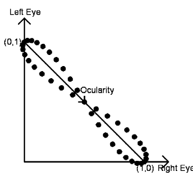
where the pure oscillation back and forth along the ocularity dimension that occurred in figure 6 develops to reveal some additional degrees of freedom, only one of which is represented in figure 7 (it is perpendicular to the ocularity axis).

If the leakage is reduced then the oscillation back and forth along the dominance axis tends to be more like a square wave than a sine wave, in which case figure 7 becomes as shown in figure 8

Figure 8: Typical neural reference vectors for low resolution input images, where reduced leakage causes the ocularity to switch abruptly back and forth.

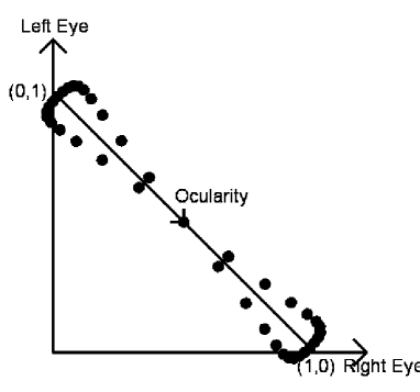
where the neural reference vectors are bunched near to the points $\left(0,1\right)$ and $\left(1,0\right)$, and explore the additional degree(s) of freedom at each end of the ocularity axis. In the extreme case, where the ocularity switches back and forth as a square wave, the neurons separate into two clusters, one of which responds only to the left retina’s image and the other to the right retina’s image. Furthermore, within each of these clusters, the neurons explore the additonal degree(s) of freedom that occur within the corresponding retina’s image. Note only one such degree of freedom is represented in figure 8; it is perpendicular to the ocularity axis.

The above arguments can be generalised to the case of input images with fine spatial structure (i.e. lots of high order terms in the Taylor expansion are required). However, more and more neurons (per receptive field) are required in order to build a faithful mapping from input space to a 2-dimensional representation in output space. For a given number of neurons (per receptive field) a saturation point will quickly be reached, where the least important detail (from the point of view of the objective function) is discarded, keeping only those properties of the input images that best preserve the ability of the neural network to reconstruct its own input with minimum Euclidean error (on average).

4 Simulations

Two types of training data will be used: synthetic, and natural. Synthetic data is used in order to demonstrate simple properties of the neural network, without introducing extraneous detail to complicate the interpretation of the results. Natural data is used to remove any doubt that the neural network is capable of producing interesting and useful results when it encounters data that is more representative of what it might encounter in the real world.

In section 4.1 dominance stripes are produced from a 1-dimensional retina, and in section 4.2 these results are generalised to a 2-dimensional retina. In both cases both synthetic and natural image results are shown. In section 4.3 orientation maps are produced for the case of two retinae trained with natural images.

4.1 Dominance Stripes: The 1-Dimensional Case

The purpose of the simulations that are presented in this section is to demonstrate the emergence of ocular dominance stripes in the simplest possible realistic case. The results will correspond to the situation outlined in figure 6.

4.1.1 Synthetic Training Data

The purpose of this simulation is to demonstrate the emergence of ocular dominance stripes, of the type that were shown in figure 6, by presenting a model of the type shown in figure 5 with very low-resolution input images. In fact, the resolution is so low that each image is entirely featureless, so that all the neurons in a retina have the same input brightness, but the two retinae have independent input brightnesses. These input images are normalised by processing them so that they look like the PMD posterior probability computed by the output layer of another such network; the neighbourhood size used for this normalisation process was chosen to be the same as the network’s own output layer neighbourhood size.

In the first simulation the parameters used were: network size = $30$, receptive field size = $9$, output layer neighbourhood size = $5$ (centred on the source neuron), leakage neighbourhood size = $5$ (centred on the source neuron), number of training updates = $2000$, update step size = $0.01$. For each neuron the leakage probability had a Gaussian profile centred on the neuron, and the standard deviation was chosen as $1$, to make the profile fall from $1$ on the source neuron to $\exp\left(-1/2\right)$ on each of its two closest neighbours.

The update scheme used was a crude gradient following algorithm parameterised by three numbers which controlled the rate at which the weight vectors, biasses and reference vectors were updated. These three numbers were continuously adjusted to ensure that the maximum rate of change (as measured over all the neurons in the network) of the length of each weight vector, and also the maximum rate of change of the absolute value of each bias, was always equal to the requested update step size; this prescription will adjust the parameter values until they jitter around in the neighbourhood of their optimum values. The optimum reference vectors could in principle be completely determined using equation 4 for each choice of weights and biasses, but it is not necessary for the reference vectors to keep in precise synchrony with the weights and biasses. Rather, the reference vectors were controlled in a similar way to the weight vectors, except that they used three times the update step size, which made them more agile than the weights and biasses they were trying to follow.

The ocular dominance stripes that emerge from this simulation are shown in figure 9. The ocularity for a given neuron was estimated by computing the average of the absolute deviations (as measured with respect to the overall mean reference vector component value, which is zero for the zero mean training data that is used here) of its reference vector components within its receptive field, both for the left retina and the right retina. This allows two plots to be drawn: average value of absolute deviations from the mean in left retina’s receptive field as a function of position across the network, and similarly the right retina’s receptive field.

Figure 9: 1-dimensional dominance stripes after training on synthetic data.

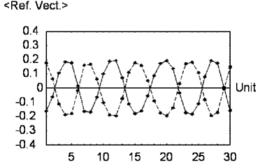
As can be seen in figure 9, these two curves are approximately periodic, and are in antiphase with each other; this corresponds to the situation shown in figure 6. The amplitude of the ocularity curves is less than the $0.5$ that would be required for the end points of the ocularity dimension to be reached, because one of the effects of leakage is to introduce a type of elastic tension between the reference vectors that causes them to contract towards zero ocularity. Note how the ocular dominance curves have a period of approximately $7$, which is slightly greater than the output layer neighbourhood size (which is $5$). In the limit of zero leakage and infinite receptive field size the period would be equal to the output layer neighbourhood size, in order to guarantee that a complete set of processing machinery is contained within each output layer neighbourhood size; this effect is called completeness.

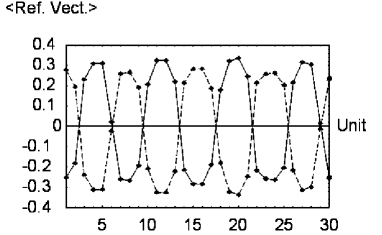
If the above simulation is continued for a further $2000$ updates with a reduced leakage, by reducing the standard deviation of the Gaussian leakage profile from $1$ to $0.5$, then the ocular dominance curves become more like square waves than sine waves, as shown in figure 10; this is similar to the type of situation that was shown in figure 8, except that the input images are featureless in this case.

Figure 10: 1-dimensional square wave dominance stripes after further training with reduced probability leakage on synthetic data.

4.1.2 Natural Training Data

Figure 11 shows the Brodatz texture image [1] that was used to generate a more realistic training set than was used in the synthetic simulations described above.

Figure 11: Brodatz texture image used as a natural training image.

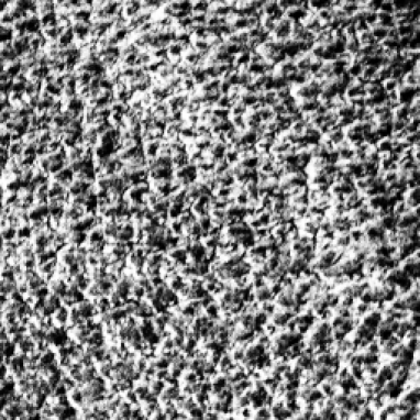
Figure 12 shows an enlarged portion of figure 11, where it is clear that the characteristic length scale of the texture structure is in the range $5-10$ pixels.

Figure 12: Magnified portion of the Brodatz texture training image.

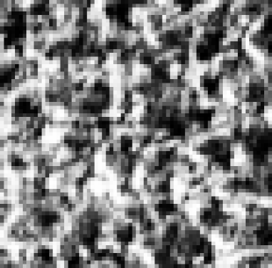
This is large enough compared to the receptive field size ($9$) and the output layer neighbourhood size ($5$) that a simulation using 1-dimensional training vectors extracted from this 2-dimensional Brodatz image will effectively see very low resolution training data, and should repond approximately as described in figure 6.

The results corresponding to figure 9 and figure 10 are shown in figure 13 and figure 14, respectively.

Figure 13: 1-dimensional dominance stripes after training on natural data.

Figure 14: 1-dimensional square wave dominance stripes after further training with reduced probability leakage on natural data.

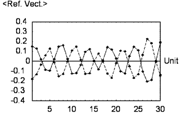
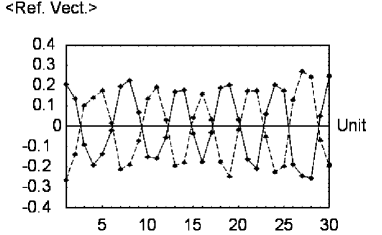
The general behaviour is much the same in the synthetic and Brodatz cases, except that the depth of the ocularity fluctuations is somewhat less in the real case, because in the Brodatz case the training data is not actually featureless within each receptive field.

4.2 Dominance Stripes: The 2-Dimensional Case

This section extends the results of the previous section to the case of 2-dimensional neural networks. The training schedule(s) used in the simulations have not been optimised. Usually the update rate is chosen conservatively (i.e. smaller than it needs to be) to avoid possible numerical instabilities, and the number of training updates is chosen to be larger than it needs to be to ensure that convergence has occurred. It is highly likely that much more efficient training schedules could be found.

4.2.1 Synthetic Training Data

The results that were presented in figure 9 may readily be extended to the case of a 2-dimensional network. The parameters used were: network size = $100\times 100$, receptive field size = $3\times 3$ (which is artificially small to allow the simulation to run faster), output layer neighbourhood size = $5\times 5$ (centred on the source neuron), leakage neighbourhood size = $3\times 3$ (centred on the source neuron), number of training updates = $24000$ (dominance stripes develop quickly, so far fewer than $24000$ training updates could be used), update step size = $0.001$. For each neuron the leakage probability had a Gaussian profile centred on the neuron, and the standard deviations were chosen as $1\times 1$, to make the profile fall from $1$ on the source neuron to $\exp\left(-1/2\right)$ on each of its four closest neighbours.

Apart from the different parameter values, the simulation was conducted in precisely the same way as in the 1-dimensional case, and the results for ocular dominance are shown in figure 15, where ocularity has been quantised as a binary-valued quantity.

Figure 15: 2-dimensional dominance stripes after training on synthetic data.

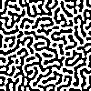
These results show the characteristic striped structure that is familiar from experiments on the mammalian visual cortex. The behaviour near to the boundary depends critically on the interplay between the receptive field size(s) and the output layer neighbourhood size(s).

4.2.2 Natural Training Data

The simulation, whose results were shown in figure 15, may be repeated using the Brodatz image training set shown in figure 11, to yield the results shown in figure 16.

Figure 16: 2-dimensional dominance stripes after training on natural data.

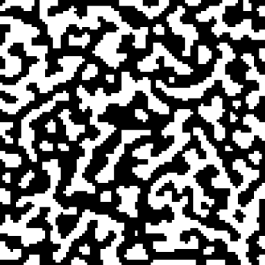
These results are not quite as stripe-like as the results in figure 15, because in the Brodatz case the training data is not actually featureless within each receptive field.

4.3 Orientation Maps

The purpose of the simulations that are presented in this section is to demonstrate the emergence of orientation maps in the simplest possible realistic case. In the case of two retinae, the results will correspond to the situation outlined in figure 7 (or, at least, a higher dimensional version of that figure).

4.3.1 Orientation Map (One Retina)

In this simulation the parameters used were: network size = $30\times 30$, receptive field size = $17\times 17$, output layer neighbourhood size = $9\times 9$ (centred on the source neuron), leakage neighbourhood size = $3\times 3$ (centred on the source neuron), number of training updates = $24000$, update step size = $0.01$. For each neuron the leakage probability had a Gaussian profile centred on the neuron, and the standard deviations were chosen as $1\times 1$, to make the profile fall from $1$ on the source neuron to $\exp\left(-1/2\right)$ on each of its four closest neighbours.

Note that both the receptive field size and the output layer neighbourhood size are substantially larger than in the 2-dimensional dominance stripe simulations, because many more neurons are required in order to allow orientation maps to develop than to allow dominance stripes to develop; in fact it would be preferable to use even larger sizes than were used here. To limit the computer run time this meant that the overall size of the neural network had to be reduced from $100\times 100$ to $30\times 30$. The training set was the Brodatz texture image in figure 11.

The results are shown in figure 17

Figure 17: Orientation map after training on natural data.

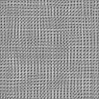
where the receptive fields have been gathered together in a montage. There is a clear swirl-like pattern that is characteristic of orientation maps. Each local clockwise or anticlockwise swirl typically circulates around an unoriented region.

4.3.2 Using the Orientation Map

In figure 18 the orientation map network shown in figure 17 is used to encode and decode a typical input image. On the left of figure 18 the input image (i.e. $\mathbf{x}$) is shown, in the centre of figure 18 the corresponding output (i.e. its PMD posterior probability $\Pr\left(y|\mathbf{x}\right)$) produced by the orientation map is shown, and on the right of figure 18 the corresponding reconstruction (i.e. $\sum_{y=1}^{M}\Pr\left(y|\mathbf{x}\right)\mathbf{x}^{\prime}\left(y\right)$) is shown.

Figure 18: Typical input, output and reconstruction produced by the orientation map.

The output consists of a number of isolated “activity bubbles” of posterior probability, and the reconstruction is a low resolution version of the original input. The form of output is familiar as a type of “sparse coding” of the input, where only a small fraction of the neurons participate in encoding a given input (this type of transformation of the input is central to the work that was reported in [13]). This type of encoding is very convenient because it has effectively transformed the input into a small number of constituents each of which corresponds to an activity bubble, rather than transforming the input into a representation where the output activity is spread over all of the neurons, which is thus not easily interpretable as arising from a small number of constituents.

The reconstruction has a lower resolution than the input because there are insufficient neurons to faithfully record all the information that is required to reconstruct the input exactly (e.g. probability leakage causes neighbouring neurons to have a correlated response, thus reducing the effective number of neurons that are available). The featureless region around the edge of the reconstruction is an artefact, which occurs because fewer neurons (per unit area) contribute to the reconstruction near the edge of the input array.

4.3.3 Orientation Map (Two Retinae)

The above orientation map results may be generalised to the case of two retinae. The parameter values used were the same, apart from the standard deviation of the leakage Gaussian which was reduced to $0.5\times 0.5$ in order to allow more detailed structure to develop in the adaptive parameter values of the output neurons. This is necessary because the presence of two retinae causes dominance stripes to develop, which allows only half of the neurons to be allocated to each retina, so a complete repertoire of computing machinery must be forced into half the number of neurons that were used in the case of one retina.

The results are shown in figure 19

Figure 19: Orientation map and dominance stripes after training on natural data.

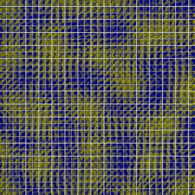
where the receptive fields for the left and right retinae have been used to create a colour separation in which one retina is coded as blue and the other as yellow. Within each retina there is a long-scale periodic fluctuation in overall brightness which corresponds to the dominance stripes. Within each dominance stripe there is the characteristic swirl-like pattern of the orientation map. Note that the unoriented regions typically occur at the centre of dominance stripes, as observed in the visual cortex; this can be understood intuitively by referring to figure 8.

A larger simulation would be required in order to accurately estimate the detailed orientation map as a vector flow field. Such simulations could be used to verify whether the iso-orientation contours typically lie perpendicular to the dominance stripe boundaries, as observed in the visual cortex. The dominance stripe structure that appears in this simulation is not as distinct as the stripes in figure 16. This is not a fundamental problem, but rather it is a result of the limited size of computer simulation that could be run in a reasonable length of time. It should also be noted that the dominance stripes that are observed in the visual cortex are sometimes more blob-like than stripe-like [14], so it is pleasing that different choices of parameter value should yield a variety of degrees of stripiness in our simulations.

5 Conclusions

This paper has shown how folded Markov chains (FMCs) [6] can be combined with partitioned mixture distributions (PMDs) [7] to yield a class of self-organising neural networks that has many of the properties that are observed in the mammalian visual cortex [2, 14], which are thus called visual cortex networks (VICON). These neural networks differ from previous models of the visual cortex, insofar as they model the neuron behaviour in terms of their individual firing events, and operate in the real space of input images rather than a hand-crafted abstract space, and the use of Bayesian methods makes the nature of the network’s computations clearer than in the case where the network behaviour is simply postulated. When the neural network structure (e.g. receptive field size) parameters are appropriately chosen, dominance stripes and orientation maps emerge naturally when the network is trained on a natural image (e.g. a Brodatz texture image).

These results show how this type of network is capable of self-organising its internal parameters in familiar ways when trained on data from multiple sources (actually, only two sources in the case of the visual cortex-like network). The same network objective function could be used when an arbitrary number of data sources is presented, and it is anticipated that it would lead to analogous results.

An extension of the network objective function to the case where sets of multiple neural firing events are considered has been published [9, 10], and an extension to the case of a multilayer network has been published [12]. When combined, these extensions could be applied to the problem of the processing of data from multiple sensors (i.e. data fusion).

Appendix A Bayesian PMD

In this section a fully Bayesian interpretation of a partitioned mixture distribution (PMD) will be presented.

Consider the general problem of computing a posterior probability $\Pr\left(y|\mathbf{x}\right)$ over classes $y$ given an input vector $\mathbf{x}$. If there is more than one model $k$ then $\Pr\left(y|\mathbf{x}\right)$ is given by a marginal PDF

$$\Pr\left(y|\mathbf{x}\right)=\sum_{k}\Pr\left(y,k|\mathbf{x}\right)$$ (23)

where $\Pr\left(y,k|\mathbf{x}\right)$ is the joint PDF of class $y$ and model $k$ given an input vector $\mathbf{x}$. Bayes’ theorem may be used to rewrite this as follows

$$\Pr\left(y,k|\mathbf{x}\right) = \frac{\Pr\left(y,k,\mathbf{x}\right)}{\Pr\left(\mathbf{x}\right)}$$ (24)

$$= \frac{\Pr\left(y|k,\mathbf{x}\right)\Pr\left(k,\mathbf{x}\right)}{\Pr\left(\mathbf{x}\right)}$$

$$= \Pr\left(y|k,\mathbf{x}\right)\Pr\left(k\right)$$

where $\Pr\left(k,\mathbf{x}\right)=\Pr\left(k\right)\Pr\left(\mathbf{x}\right)$ (i.e. independence of model $k$ and data vector $\mathbf{x}$) has been assumed in the last step. Thus the posterior probability $\Pr\left(y|\mathbf{x}\right)$ may be written as

$$\Pr\left(y|\mathbf{x}\right)=\sum_{k}\Pr\left(y|k,\mathbf{x}\right)\Pr\left(k\right)$$ (25)

Assume that there are $M$ models, and that the prior probabilities $\Pr\left(k\right)$ of the various models are equal, so that $\Pr\left(k\right)=\frac{1}{M}$, in which case the posterior probability reduces to

$$\Pr\left(y|\mathbf{x}\right)=\frac{1}{M}\sum_{k=1}^{M}\Pr\left(y|k,\mathbf{x}\right)$$ (26)

which is an average of $M$ contributing posterior probabilities (one from each of the contributing models). The PMD posterior probability in equation 8 is a special case of this result.

More generally, the prior probabilities $\Pr\left(k\right)$ are $k$-dependent, and might be chosen in some optimal fashion to best handle the training set. The simplest way of determining an optimal $\Pr\left(k\right)$ is to minimise $D$ with respect to $\Pr\left(k\right)$; this merely extends the space in which $D$ is optimised to include more of the parameters inside $\Pr\left(y|\mathbf{x}\right)$.

Appendix B Optimal Solutions

In this section the the objective function $D$ will be minimised in the case where the input space consists of one or more subspaces, within each of which all of the input vector components have the same value. In the language of imaging sensors, these special cases correspond to each sensor viewing a featureless scene (i.e. all pixels having the same brightness value), which is effectively the lowest order term in a Taylor expansion of the spatial variation of pixel brightness values. This might not appear to be an interesting scenario to consider, but it leads to a highly non-trivial optimal network behaviour when $D$ is minimised. More complicated input statistics leads to even more complicated optimal network behaviour, so only the simplest case described above will be considered at first.

B.1 One Input Subspace

This may be used to optimise the network for a single sensor viewing a featureless scene. For a $d$-dimensional input space $\Pr\left(\mathbf{x}\right)$ is thus given by

$$\Pr\left(\mathbf{x}\right)=\Pr\left(x_{1}\right)\prod_{i=2}^{d}\delta\left(x_{i}-x_{1}\right)$$ (27)

whence the objective function $D$ in equation 3 reduces to

$$D=2d\int dx_{1}\Pr\left(x_{1}\right)\sum_{y=1}^{M}\Pr\left(y|x_{1}\right)\left(x_{1}-x_{1}^{\prime}\left(y\right)\right)^{2}$$ (28)

This is $d$ times the objective function for a 1-dimensional soft scalar quantiser which encodes inputs in $x_{1}$-space whose PDF is $\Pr\left(x_{1}\right)$.

B.2 Two Input Subspaces

This may be used to optimise the network for a pair of sensors each of which views a featureless scene, and which are possibly correlated with each other. The one input subspace case above can readily be generalised to more input subspaces. Let the $d$-dimensional input space be split into two $\frac{d}{2}$-dimensional subspaces, where $\Pr\left(\mathbf{x}\right)$ is given by

$$\Pr\left(\mathbf{x}\right)=\Pr\left(x_{1},x_{2}\right)\prod_{i=2}^{\frac{d}{2}}\delta\left(x_{2\bar{\imath}-1}-x_{1}\right)\delta\left(x_{2\bar{\imath}}-x_{2}\right)$$ (29)

where one of the subspaces consists of the odd-numbered components, and the other the even-numbered components of the input vector (this particular ordering of the components is not important). Whence the objective function $D$ in equation 3 reduces to

$$D = d\int dx_{1}dx_{2}\Pr\left(x_{1},x_{2}\right)\sum_{y=1}^{M}\Pr\left(y|x_{1},x_{2}\right)$$ (30)

$$\times\left(\left(x_{1}-x_{1}^{\prime}\left(y\right)\right)^{2}+\left(x_{2}-x_{2}^{\prime}\left(y\right)\right)^{2}\right)$$

This is $\frac{d}{2}$ times the objective function for a 2-dimensional soft vector quantiser which encodes inputs in $\left(x_{1},x_{2}\right)$-space whose PDF is $\Pr\left(x_{1},x_{2}\right)$. This result generalises in the obvious way to a larger number of input subspaces.

B.3 PMD Posterior Probability

In the above special cases each neuron potentially responds to all of the components of the input vector. If this were to be built in hardware, then each neuron would have a number of inputs equal to the dimensionality of the input space, which becomes unwieldy if the input space had a high dimensionality (e.g. an image). For high-dimensional inputs it is sensible to limit the number of inputs to each neuron, which can readily be implemented by imposing a finite-sized receptive field on the input of each neuron, such that it can respond only to a limited subset of all of the input vector components. This constraint will prevent the ideal vector quantiser solutions from being obtained, so the purpose of this section is to derive the constrained optimal solution. Note that this type of input is a special case of the type of solution that would be obtained by adding a “wire-length” penalty term to the objective function in order to penalise the connection of a neuron to too many input components.

Even if receptive fields are used to restrict the length of the input connections, the posterior probability $\Pr\left(y|\mathbf{x}\right)$ effectively needs long-range lateral connections between the output neurons in order to implement the normalisation condition $\sum_{y=1}^{M}\Pr\left(y|\mathbf{x}\right)=1$. The simplest example of this is the standard vector quantiser, whose winner-take-all property requires that all neurons are laterally connected to all other neurons even if each of them has only a finite-sized receptive field. A partitioned mixture distribution (PMD) posterior probability, in which the posterior probability $\Pr\left(y|\mathbf{x}\right)$ is only locally connected, can be used to ensure that all the connections in the network are local (see section 2.3).

B.3.1 Receptive Fields

Write the input vector as $\mathbf{x=}\left(\mathbf{\tilde{x}}\left(y\right),\mathbf{\bar{x}}\left(y\right)\right)$ where $\mathbf{\tilde{x}}\left(y\right)$ is the part of $\mathbf{x}$ that lies within the receptive field of neuron $y$, and, for simplicity, assume that the receptive field used for $\mathbf{x}^{\prime}\left(y\right)$ is chosen to be the same as that for $\mathbf{\tilde{x}}\left(y\right)$, and that all receptive fields see the same number $w$ of input components. Because the input vector is split into two subspaces as $\mathbf{x}=\left(\mathbf{x}_{1},\mathbf{x}_{2}\right)$, its decompositon as $\left(\mathbf{\tilde{x}}\left(y\right),\mathbf{\bar{x}}\left(y\right)\right)$ may similarly be split into two subspaces as $\mathbf{\tilde{x}}\left(y\right)=\left(\mathbf{\tilde{x}}_{1}\left(y\right),\mathbf{\tilde{x}}_{2}\left(y\right)\right)$ and $\mathbf{\bar{x}}\left(y\right)=\left(\mathbf{\bar{x}}_{1}\left(y\right),\mathbf{\bar{x}}_{2}\left(y\right)\right)$. Use the orthogonality of $\mathbf{\tilde{x}}\left(y\right)$ and $\mathbf{\bar{x}}\left(y\right)$ to write (for $i=1,2$)

$$\left\|\mathbf{\bar{x}}_{i}\left(y\right)+\mathbf{\tilde{x}}_{i}\left(y\right)-\mathbf{x}_{i}^{\prime}\left(y\right)\right\|^{2}=\left\|\mathbf{\bar{x}}_{i}\left(y\right)\right\|^{2}+\left\|\mathbf{\tilde{x}}_{i}\left(y\right)-\mathbf{x}_{i}^{\prime}\left(y\right)\right\|^{2}$$

and simplify $D$ in equation 3 thus

$$D = 2\int d\mathbf{x}_{1}d\mathbf{x}_{2}\Pr\left(\mathbf{x}_{1},\mathbf{x}_{2}\right)\sum_{y}\Pr\left(y|\mathbf{x}_{1},\mathbf{x}_{2}\right)$$ (33)

$$\times\left(\begin{array}[]{c}\left\|\mathbf{\bar{x}}_{1}\left(y\right)\right\|^{2}+\left\|\mathbf{\bar{x}}_{2}\left(y\right)\right\|^{2}\\ +\left\|\mathbf{\tilde{x}}_{1}\left(y\right)-\mathbf{x}_{1}^{\prime}\left(y\right)\right\|^{2}+\left\|\mathbf{\tilde{x}}_{2}\left(y\right)-\mathbf{x}_{2}^{\prime}\left(y\right)\right\|^{2}\end{array}\right)$$

There are two terms to consider.

1. $\left\|\mathbf{\bar{x}}_{1}\left(y\right)\right\|^{2}+\left\|\mathbf{\bar{x}}_{2}\left(y\right)\right\|^{2}$. This is the contribution from outside the $y^{th}$ receptive field, which is the $L_{2}$ norm of those components of the input vector that lie outside the $y^{th}$ receptive field.

2. $\left\|\mathbf{\tilde{x}}_{1}\left(y\right)-\mathbf{x}_{1}^{\prime}\left(y\right)\right\|^{2}+\left\|\mathbf{\tilde{x}}_{2}\left(y\right)-\mathbf{x}_{2}^{\prime}\left(y\right)\right\|^{2}$: This is the contribution from inside the $y^{th}$ receptive field, which is the $L_{2}$ norm of those components of the error vector (i.e. input minus reconstruction) that lie inside the $y^{th}$ receptive field.

B.3.2 Simplify the $\left\|\mathbf{\bar{x}}_{1}\left(y\right)\right\|^{2}+\left\|\mathbf{\bar{x}}_{2}\left(y\right)\right\|^{2}$ Term

$\left\|\mathbf{\bar{x}}_{1}\left(y\right)\right\|^{2}+\left\|\mathbf{\bar{x}}_{2}\left(y\right)\right\|^{2}$ is the $L_{2}$ norm of those components of the input vector that lie outside the $y^{th}$ receptive field, which is known once the input vector is specified. Furthermore, because of the assumed input PDF (i.e. all input components in each subspace have the same value), together with the assumed receptive field prescription (i.e. all receptive fields are the same size $w$), this $L_{2}$ norm is independent of $y$ given that $\mathbf{x}$ is known, so this term has the following contribution to $D$

$$D=\left(d-w\right)\left(\int dx_{1}\Pr\left(x_{1}\right)x_{1}^{2}+\int dx_{2}\Pr\left(x_{2}\right)x_{2}^{2}\right)$$ (34)

where $d-w$ is the number of input components that lie outside each receptive field.

B.3.3 Simplify the $\left\|\mathbf{\tilde{x}}_{1}\left(y\right)-\mathbf{x}_{1}^{\prime}\left(y\right)\right\|^{2}+\left\|\mathbf{\tilde{x}}_{2}\left(y\right)-\mathbf{x}_{2}^{\prime}\left(y\right)\right\|^{2}$ Term

Assume that $\Pr\left(y|\mathbf{x}_{1},\mathbf{x}_{2}\right)$ has the PMD form of a sum over mixture distribution posterior probabilities (as described in section 2.3), so that

$$\Pr\left(y|\mathbf{x}_{1},\mathbf{x}_{2}\right) = \frac{1}{M}\sum_{y^{\prime}\in\mathcal{N}^{-1}\left(y\right)}\Pr\left(y|\mathbf{x}_{1},\mathbf{x}_{2}\mathbf{;}y^{\prime}\right)$$ (35)

$$= \frac{1}{M}\,Q\left(\mathbf{\tilde{x}}_{1},\mathbf{\tilde{x}}_{2}\mathbf{|}y\right)\sum_{y^{\prime}\in\mathcal{N}^{-1}\left(y\right)}\frac{1}{\sum_{y^{\prime\prime}\in\mathcal{N}\left(y^{\prime}\right)}Q\left(\mathbf{\tilde{x}}_{1},\mathbf{\tilde{x}}_{2}\mathbf{|}y^{\prime\prime}\right)}$$

The overall receptive field that effects the value of $\Pr\left(y|\mathbf{x}_{1},\mathbf{x}_{2}\right)$ (for a given $y$) may be read off this expression. Thus $\mathbf{\tilde{x}}\left(y^{\prime\prime}\right)$ comprises those components of $\mathbf{x}$ that lie within the receptive field of neuron $y^{\prime\prime}$, and the $\sum_{y^{\prime}\in\mathcal{N}^{-1}\left(y\right)}\frac{1}{\sum_{y^{\prime\prime}\in\mathcal{N}\left(y^{\prime}\right)}\left(\cdots\right)}$ operation compounds these $\mathbf{\tilde{x}}\left(y^{\prime\prime}\right)$ so that the overall set of components of $\mathbf{x}$ that are needed for the purposes of calculating $\Pr\left(y|\mathbf{x}_{1},\mathbf{x}_{2}\right)$ is given by (using a somewhat cavalier notation)

$$\mathbf{\tilde{X}}\left(y\right)\equiv\bigcup_{y^{\prime}\in\mathcal{N}^{-1}\left(y\right)}\bigcup_{y^{\prime\prime}\in\mathcal{N}\left(y^{\prime}\right)}\mathbf{\tilde{x}}\left(y^{\prime\prime}\right)$$ (36)

The individual $\Pr\left(y|\mathbf{x}_{1},\mathbf{x}_{2}\mathbf{;}y^{\prime}\right)$ that contribute to $\Pr\left(y|\mathbf{x}_{1},\mathbf{x}_{2}\right)$ each depend on a smaller set of components of $\mathbf{x}$ than the full $\Pr\left(y|\mathbf{x}_{1},\mathbf{x}_{2}\right)$, because there is one less summation over a $y$ variable. However, it is convenient, and imposes no constraint, to use the full set of components thus

$$\Pr\left(y|\mathbf{x}_{1},\mathbf{x}_{2};y^{\prime}\right)=\Pr\left(y|\mathbf{\tilde{X}}_{1}\left(y\right),\mathbf{\tilde{X}}_{2}\left(y\right);y^{\prime}\right)$$ (37)

The $y$ and $y^{\prime}$ summations can be interchanged using $\sum_{y=1}^{M}\sum_{y^{\prime}\in\mathcal{N}^{-1}\left(y\right)}\left(\cdots\right)=\sum_{y^{\prime}=1}^{M}\sum_{y\in\mathcal{N}\left(y^{\prime}\right)}\left(\cdots\right)$, whence the contribution to $D$ is

$$D = \frac{2}{M}\int d\mathbf{x}_{1}\,d\mathbf{x}_{2}\Pr\left(\mathbf{x}_{1},\mathbf{x}_{2}\right)\sum_{y^{\prime}=1}^{M}\sum_{y\in\mathcal{N}\left(y^{\prime}\right)}\Pr\left(y|\mathbf{\tilde{X}}_{1}\left(y\right),\mathbf{\tilde{X}}_{2}\left(y\right);y^{\prime}\right)$$ (38)

$$\times\left(\left\|\mathbf{\tilde{x}}_{1}\left(y\right)-\mathbf{x}_{1}^{\prime}\left(y\right)\right\|^{2}+\left\|\mathbf{\tilde{x}}_{2}\left(y\right)-\mathbf{x}_{2}^{\prime}\left(y\right)\right\|^{2}\right)$$

Because the components of $\mathbf{\tilde{x}}_{i}\left(y\right)$ are a subset of the components of $\mathbf{\tilde{X}}_{i}\left(y\right)$(for $i=1,2$), $\Pr\left(\mathbf{x}_{1},\mathbf{x}_{2}\right)$ can be marginalised to yield

$$D = \frac{2}{M}\sum_{y^{\prime}=1}^{M}\sum_{y\in\mathcal{N}\left(y^{\prime}\right)}\int d\mathbf{\tilde{X}}_{1}\left(y\right)\,d\mathbf{\tilde{X}}_{2}\left(y\right)\Pr\left(\mathbf{\tilde{X}}_{1}\left(y\right),\mathbf{\tilde{X}}_{2}\left(y\right)\right)$$ (39)

$$\times\Pr\left(y|\mathbf{\tilde{X}}_{1}\left(y\right),\mathbf{\tilde{X}}_{2}\left(y\right);y^{\prime}\right)$$

$$\times\left(\left\|\mathbf{\tilde{x}}_{1}\left(y\right)-\mathbf{x}_{1}^{\prime}\left(y\right)\right\|^{2}+\left\|\mathbf{\tilde{x}}_{2}\left(y\right)-\mathbf{x}_{2}^{\prime}\left(y\right)\right\|^{2}\right)$$

Because $\Pr\left(\mathbf{x}_{1},\mathbf{x}_{2}\right)$ specifies that all of the components in each subspace are the same, this contribution to $D$ may be simplified to

$$D = \frac{w}{M}\sum_{y^{\prime}=1}^{M}\sum_{y\in\mathcal{N}\left(y^{\prime}\right)}\int dx_{1}\,dx_{2}\Pr\left(x_{1},x_{2}\right)\Pr\left(y|x_{1},x_{2};y^{\prime}\right)$$ (40)

$$\times\left(\left(x_{1}-x_{1}^{\prime}\left(y\right)\right)^{2}+\left(x_{2}-x_{2}^{\prime}\left(y\right)\right)^{2}\right)$$

B.3.4 Periodic Optimal Solutions

Combining the results from outside (equation 34) and inside (equation 40) the receptive fields yields finally

$$D = \left(d-w\right)\left(\int dx_{1}\Pr\left(x_{1}\right)x_{1}^{2}+\int dx_{2}\Pr\left(x_{2}\right)x_{2}^{2}\right)$$ (41)

$$+\frac{w}{M}\sum_{y^{\prime}=1}^{M}\sum_{y\in\mathcal{N}\left(y^{\prime}\right)}\int dx_{1}\,dx_{2}\Pr\left(x_{1},x_{2}\right)\Pr\left(y|x_{1},x_{2};y^{\prime}\right)$$

$$\times\left(\left(x_{1}-x_{1}^{\prime}\left(y\right)\right)^{2}+\left(x_{2}-x_{2}^{\prime}\left(y\right)\right)^{2}\right)$$

The first of these terms is constant, so it may be ignored insofar as network optimisation is concerned. The second term is much more interesting. It is the sum of the objective functions of a large number of 2-dimensional soft vector quantisers. However, these objective functions cannot be optimised independently of each other, because the posterior probabilities $\Pr\left(y|x_{1},x_{2};y^{\prime}\right)$ force the neurons to share parameters with each other.

Drop the constant term, and interchange the order of summation to obtain

$$D = w\sum_{y=1}^{M}\int dx_{1}\,dx_{2}\Pr\left(x_{1},x_{2}\right)\Pr\left(y|x_{1},x_{2}\right)$$ (42)

$$\times\left(\left(x_{1}-x_{1}^{\prime}\left(y\right)\right)^{2}+\left(x_{2}-x_{2}^{\prime}\left(y\right)\right)^{2}\right)$$

where $\Pr\left(y|x_{1},x_{2}\right)$ is the PMD posterior probability given by

$$\Pr\left(y|x_{1},x_{2}\right)=\frac{1}{M}\sum_{y^{\prime}\in\mathcal{N}^{-1}\left(y\right)}\Pr\left(y|x_{1},x_{2};y^{\prime}\right)$$ (43)

Now suppose that $\Pr\left(y|x_{1},x_{2}\right)$ and $x_{i}^{\prime}\left(y\right)$ have the periodicity property

$$\Pr\left(y+m|x_{1},x_{2}\right) = \Pr\left(y|x_{1},x_{2}\right)$$

$$x_{i}^{\prime}\left(y+m\right) = x_{i}^{\prime}\left(y\right)$$ (44)

where the fact that $y$ is restricted to $1\leq y\leq M$ has been ignored for simplicity, then $D$ can be simplified thus (again, ignoring the fact that $y$ is restricted to $1\leq y\leq M$)

$$D = w\sum_{y_{0}=0}^{\frac{M}{m}-1}\sum_{y=my_{0}+1}^{m\left(y_{0}+1\right)}\int dx_{1}\,dx_{2}\Pr\left(x_{1},x_{2}\right)\Pr\left(y|x_{1},x_{2}\right)$$ (45)

$$\times\left(\left(x_{1}-x_{1}^{\prime}\left(y\right)\right)^{2}+\left(x_{2}-x_{2}^{\prime}\left(y\right)\right)^{2}\right)$$

$$= w\sum_{y=1}^{m}\int dx_{1}\,dx_{2}\Pr\left(x_{1},x_{2}\right)\frac{M}{m}\Pr\left(y|x_{1},x_{2}\right)$$

$$\times\left(\left(x_{1}-x_{1}^{\prime}\left(y\right)\right)^{2}+\left(x_{2}-x_{2}^{\prime}\left(y\right)\right)^{2}\right)$$

where $\frac{M}{m}\sum_{y=1}^{m}\Pr\left(y|x_{1},x_{2}\right)=1$ follows from $\sum_{y=1}^{M}\Pr\left(y|x_{1},x_{2}\right)=1$ and the periodicity property, so $\frac{M}{m}\Pr\left(y|x_{1},x_{2}\right)$ serves as a posterior probability for $1\leq y\leq m$.

This demonstrates that if the optimal solution is periodic, with period $m$, then the objective function is proportional to the objective function for a 2-dimensional soft vector quantiser with $m$ neurons. Note that thus far nothing has been said about the actual value of $m$; its optimal value depends on the interplay between the receptive field size(s), the output layer neighbourhood size(s), and the leakage neighbourhood size(s). Because this type of periodic solution is essentially a set of overlapping $m$ neuron soft vector quantisers, each set of $m$ neurons will typically exhibit the properties of such quantisers. In particular this means that each set of $m$ neurons will have the means to encode and (approximately) reconstruct those components of the input vector that it sees via its receptive fields.

This type of solution is the archetype for orientation maps, where the neurons arrange their properties so that each local patch (corresponding to the $m$ neurons in the periodic solution derived above) has the means to encode whatever orientation of object it sees via its receptive fields. The full derivation of an orientation map would require a more sophisticated analysis than the simple 1-dimensional case derived above.

References

- [1] Brodatz P, 1966, Textures - a photographic album for artists and designers, Dover.
- [2] Goodhill G, 1992, CSRP 226, University of Sussex, Correlations, competition and optimality: modelling the development of topography and ocular dominance.
- [3] Kohonen T, 1984, Springer-Verlag, Self-organisation and associative memory.
- [4] Linde Y, Buzo A and Gray R M, 1980, IEEE Trans. COM, 28, 84-95 An algorithm for vector quantiser design.
- [5] Luttrell S P, 1990, IEEE Transactions on Neural Networks, 1, 229-232, Derivation of a class of training algorithms.
- [6] Luttrell S P, 1994, Neural Computation, 6, 767-794, A Bayesian analysis of self-organising maps.
- [7] Luttrell S P, 1994, Proc. IEE Vision, Image and Signal Processing, 141, 251-260, The partitioned mixture distribution: an adaptive Bayesian network for low-level image processing.
- [8] Luttrell S P, 1994, Proc. 14th Int. MAXENT Workshop, 279-286, Kluwer, The partitioned mixture distribution: multiple overlapping density models.
- [9] Luttrell S P, 1996, Handbook of Neural Computation, section B5.3, OUP, Designing analysable networks.
- [10] Luttrell S P, 1996, to appear in the Proceedings of the 1st Conference on Mathematics of Artificial Neural Networks and Applications (in Annals of Mathematics and Artificial Intelligence), Oxford, A theory of self-organising neural networks.
- [11] Luttrell S P, 1995, DRA Report, DRA/CIS(SE1)/651/11/RP/1.1, A self-organising network for processing data from multiple sensors.
- [12] Luttrell S P, 1996, Network, 7, 285-290, A discrete firing event analysis of the adaptive cluster expansion network.
- [13] Webber C J S, 1994, Network, 5, 471-495, Self-organisation of transformation-invariant detectors for constituents of perceptual patterns.
- [14] Swindale N V, 1996, Network, 7, 161-247, The development of topography in the visual cortex: a review of models.