Stochastic Vector Quantisers

Abstract: In this paper a stochastic generalisation of the standard Linde-Buzo-Gray (LBG) approach to vector quantiser (VQ) design is presented, in which the encoder is implemented as the sampling of a vector of code indices from a probability distribution derived from the input vector, and the decoder is implemented as a superposition of reconstruction vectors, and the stochastic VQ is optimised using a minimum mean Euclidean reconstruction distortion criterion, as in the LBG case. Numerical simulations are used to demonstrate how this leads to self-organisation of the stochastic VQ, where different stochastically sampled code indices become associated with different input subspaces. This property may be used to automate the process of splitting high-dimensional input vectors into low-dimensional blocks before encoding them.

1 Introduction

In vector quantisation a code book is used to encode each input vector as a corresponding code index, which is then decoded (again, using the codebook) to produce an approximate reconstruction of the original input vector [3, 2]. The purpose of this paper is to generalise the standard approach to vector quantiser (VQ) design [7], so that each input vector is encoded as a vector of code indices that are stochastically sampled from a probability distribution that depends on the input vector, rather than as a single code index that is the deterministic outcome of finding which entry in a code book is closest to the input vector. This will be called a stochastic VQ (SVQ), and it includes the standard VQ as a special case. Note that this approach is different from the various soft competition and stochastic relaxation schemes that are used to train VQs (see e.g. [13]), because here the probability distribution is an essential part of the encoder, both during and after training.

One advantage of using the stochastic approach, which will be demonstrated in this paper, is that it automates the process of splitting high-dimensional input vectors into low-dimensional blocks before encoding them, because minimising the mean Euclidean reconstruction error can encourage different stochastically sampled code indices to become associated with different input subspaces [10]. Another advantage is that it is very easy to connect SVQs together, by using the vector of code index probabilities computed by one SVQ as the input vector to another SVQ [11].

In section 2 various pieces of previously published theory are unified to give a coherent account of SVQs. In section 3 the results of some new numerical simulations are presented, which demonstrate how the code indices in a SVQ can become associated in various ways with input subspaces.

2 Theory

In this section various pieces of previously published theory are unified to establish a coherent framework for modelling SVQs.

In section 2.1 the basic theory of folded Markov chains (FMC) is given [8], and in section 2.2 it is extended to the case of high-dimensional input data [9]. In section 2.3 some properties of the solutions that emerge when the input vector lives on a 2-torus are summarised [10]. Finally, in section 2.4 the theory is further generalised to chains of linked FMCs [11].

2.1 Folded Markov Chains

The basic building block of the encoder/decoder model used in this paper is the folded Markov chain (FMC) [8]. Thus an input vector $\mathbf{x}$ is encoded as a code index vector $\mathbf{y}$, which is then subsequently decoded as a reconstruction $\mathbf{x}^{\prime}$ of the input vector. Both the encoding and decoding operations are allowed to be probabilistic, in the sense that $\mathbf{y}$ is a sample drawn from $\Pr\left(\mathbf{y}|\mathbf{x}\right)$, and $\mathbf{x}^{\prime}$ is a sample drawn from $\Pr\left(\mathbf{x}^{\prime}|\mathbf{y}\right)$, where $\Pr\left(\mathbf{y}|\mathbf{x}\right)$ and $\Pr\left(\mathbf{x}|\mathbf{y}\right)$ are Bayes’ inverses of each other, as given by

$$\Pr\left(\mathbf{x}|\mathbf{y}\right)=\frac{\Pr\left(\mathbf{y}|\mathbf{x}\right)\Pr\left(\mathbf{x}\right)}{\int d\mathbf{z}\Pr\left(\mathbf{y}|\mathbf{z}\right)\Pr\left(\mathbf{z}\right)}$$ (1)

and $\Pr\left(\mathbf{x}\right)$ is the prior probability from which $\mathbf{x}$ was sampled.

Because the chain of dependences in passing from $\mathbf{x}$ to $\mathbf{y}$ and then to $\mathbf{x}^{\prime}$ is first order Markov (i.e. it is described by the directed graph $\mathbf{x}\longrightarrow\mathbf{y}\longrightarrow\mathbf{x}^{\prime}$), and because the two ends of this Markov chain (i.e. $\mathbf{x}$ and $\mathbf{x}^{\prime}$) live in the same vector space, it is called a folded Markov chain (FMC). The operations that occur in an FMC are summarised in figure 1.

Figure 1: A folded Markov chain (FMC) in which an input vector $\mathbf{x}$ is encoded as a code index vector $\mathbf{y}$ that is drawn from a conditional probability $\Pr\left(\mathbf{y}|\mathbf{x}\right)$, which is then decoded as a reconstruction vector $\mathbf{x}^{\prime}$ drawn from the Bayes’ inverse conditional probability $\Pr\left(\mathbf{x}^{\prime}|\mathbf{y}\right)$.

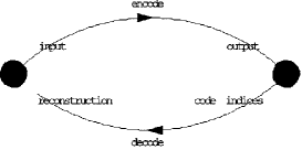
In order to ensure that the FMC encodes the input vector optimally, a measure of the reconstruction error must be minimised. There are many possible ways to define this measure, but one that is consistent with many previous results, and which also leads to many new results, is the mean Euclidean reconstruction error measure $D$, which is defined as

$$D\equiv\int d\mathbf{x}\Pr\left(\mathbf{x}\right)\sum_{\mathbf{y}=1}^{\mathbf{M}}\Pr\left(\mathbf{y}|\mathbf{x}\right)\int d\mathbf{x}^{\prime}\Pr\left(\mathbf{x}^{\prime}|\mathbf{y}\right)\left\|\mathbf{x}-\mathbf{x}^{\prime}\right\|^{2}$$ (2)

where $\Pr\left(\mathbf{x}\right)\Pr\left(\mathbf{y}|\mathbf{x}\right)\Pr\left(\mathbf{x}^{\prime}|\mathbf{y}\right)$ is the joint probability that the FMC has state $\left(\mathbf{x},\mathbf{y},\mathbf{x}^{\prime}\right)$, $\left\|\mathbf{x}-\mathbf{x}^{\prime}\right\|^{2}$ is the Euclidean reconstruction error, and $\int d\mathbf{x}\sum_{\mathbf{y}=1}^{\mathbf{M}}\int d\mathbf{x}^{\prime}\left(\cdots\right)$ sums over all possible states of the FMC (weighted by the joint probability). The code index vector $\mathbf{y}$ is assumed to lie on a rectangular lattice of size $\mathbf{M}$.

The Bayes’ inverse probability $\Pr\left(\mathbf{x}^{\prime}|\mathbf{y}\right)$ may be integrated out of this expression for $D$ to yield

$$D=2\int d\mathbf{x}\Pr\left(\mathbf{x}\right)\sum_{\mathbf{y}=1}^{\mathbf{M}}\Pr\left(\mathbf{y}|\mathbf{x}\right)\left\|\mathbf{x}-\mathbf{x}^{\prime}\left(\mathbf{y}\right)\right\|^{2}$$ (3)

where the reconstruction vector $\mathbf{x}^{\prime}\left(\mathbf{y}\right)$ is defined as $\mathbf{x}^{\prime}\left(\mathbf{y}\right)\equiv\int d\mathbf{x}\Pr\left(\mathbf{x}|\mathbf{y}\right)\,\mathbf{x}$. Because of the quadratic form of the objective function, it turns out that $\mathbf{x}^{\prime}\left(\mathbf{y}\right)$ may be treated as a free parameter whose optimum value (i.e. the solution of $\frac{\partial D}{\partial\mathbf{x}^{\prime}\left(\mathbf{y}\right)}=0$) is $\int d\mathbf{x}\Pr\left(\mathbf{x}|\mathbf{y}\right)\,\mathbf{x}$, as required.

If $D$ is now minimised with respect to the probabilistic encoder $\Pr\left(\mathbf{y}|\mathbf{x}\right)$ and the reconstruction vector $\mathbf{x}^{\prime}\left(\mathbf{y}\right)$, then the optimum has the form

$$\Pr\left(\mathbf{y}|\mathbf{x}\right) = \delta_{\mathbf{y},\mathbf{y}\left(\mathbf{x}\right)}$$

$$\mathbf{y}\left(\mathbf{x}\right) = \begin{array}[]{c}\arg\min\\ \mathbf{y}\end{array}\left\|\mathbf{x}-\mathbf{x}^{\prime}\left(\mathbf{y}\right)\right\|^{2}$$ (6)

$$\mathbf{x}^{\prime}\left(\mathbf{y}\right) = \int d\mathbf{x}\Pr\left(\mathbf{x}|\mathbf{y}\right)\,\mathbf{x}$$ (7)

where $\Pr\left(\mathbf{y}|\mathbf{x}\right)$ has reduced to a deterministic encoder (as described by the Kronecker delta $\delta_{\mathbf{y},\mathbf{y}\left(\mathbf{x}\right)}$), $\mathbf{y}\left(\mathbf{x}\right)$ is a nearest neighbour encoding algorithm using code vectors $\mathbf{x}^{\prime}\left(\mathbf{y}\right)$ to partition the input space into code cells, and (in an optimised configuration) the $\mathbf{x}^{\prime}\left(\mathbf{y}\right)$ are the centroids of these code cells. This is equivalent to a standard VQ [7].

An extension of the standard VQ to the case of where the code index is transmitted along a noisy communication channel before the reconstruction is attempted [6, 1] was derived in [8], and was shown to lead to a good approximation to a topographic mapping neural network [5].

2.2 High Dimensional Input Spaces

A problem with the standard VQ is that its code book grows exponentially in size as the dimensionality of the input vector is increased, assuming that the contribution to the reconstruction error from each input dimension is held constant. This means that such VQs are useless for encoding extremely high dimensional input vectors, such as images. The usual solution to this problem is to partition the input space into a number of lower dimensional subspaces (or blocks), and then to encode each of these subspaces separately. However, this produces an undesirable side effect, where the boundaries of the blocks are clearly visible in the reconstruction; this is the origin of the blocky appearance of reconstructed images, for instance.

There is also a much more fundamental objection to this type of partitioning, because the choice of blocks should ideally be decided in such a way that the correlations within a block are much stronger than the correlations between blocks. In the case of image encoding, this will usually be the case if the partitioning is that each block consists of contiguous image pixels. However, more generally, there is no guarantee that the input vector statistics will respect the partitioning in this convenient way. Thus it will be necessary to deduce the best choice of blocks from the training data.

In order to solve the problem of finding the best partitioning, consider the following constraint on $\Pr\left(\mathbf{y}|\mathbf{x}\right)$ and $\mathbf{x}^{\prime}\left(\mathbf{y}\right)$ in the FMC objective function in equation 3

$$\mathbf{y} = \left(y_{1},y_{2},\cdots,y_{n}\right),1\leq y_{i}\leq M$$

$$\Pr\left(\mathbf{y}|\mathbf{x}\right) = \Pr\left(y_{1}|\mathbf{x}\right)\Pr\left(y_{2}|\mathbf{x}\right)\cdots\Pr\left(y_{n}|\mathbf{x}\right)$$

$$\mathbf{x}^{\prime}\left(\mathbf{y}\right) = \frac{1}{n}\sum_{i=1}^{n}\mathbf{x}^{\prime}\left(y_{i}\right)$$ (8)

Thus the code index vector $\mathbf{y}$ is assumed to be $n$-dimensional, each component $y_{i}$ (for $i=1,2,\cdots,n$ and $1\leq y_{i}\leq M$) is an independent sample drawn from $\Pr(y|\mathbf{x})$, and the reconstruction vector $\mathbf{x}^{\prime}\left(\mathbf{y}\right)$ (vector argument) is assumed to be a superposition of $n$ contributions $\mathbf{x}^{\prime}\left(y_{i}\right)$ (scalar argument) for $i=1,2,\cdots,n$. As $D$ is minimised, this constraint allows partitioned solutions to emerge by a process of self-organisation.

For instance, solutions can have the structure illustrated in figure 2.

Figure 2: A typical solution in which the components of the input vector $\mathbf{x}$ and the range of values of the output code index $y$ are both partitioned into blocks. These input and output blocks are connected together as illustrated. More generally, the blocks may overlap each other.

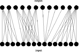
This type of structure is summarised as follows

$$\mathbf{x} = \left(\mathbf{x}_{1},\mathbf{x}_{2},\cdots,\mathbf{x}_{N}\right)$$

$$\Pr\left(\mathbf{y}|\mathbf{x}\right) = \Pr\left(y_{1}|\mathbf{x}_{p\left(y_{1}\right)}\right)\Pr\left(y_{2}|\mathbf{x}_{p\left(y_{2}\right)}\right)\,\cdots\,\Pr\left(y_{n}|\mathbf{x}_{p\left(y_{n}\right)}\right)$$ (9)

In this type of solution the input vector $\mathbf{x}$ is partitioned as $\left(\mathbf{x}_{1},\mathbf{x}_{2},\cdots,\mathbf{x}_{N}\right)$, the probability $\Pr\left(y|\mathbf{x}\right)$ reduces to $\Pr\left(y|\mathbf{x}_{p\left(y\right)}\right)$ which depends only on $\mathbf{x}_{p\left(y\right)}$, where the function $p\left(y\right)$ computes the index of the block which code index $y$ inhabits. There is not an exact correspondence between this type of partitioning and that used in the standard approach to encoding image blocks, because here the $n$ code indices are spread at random over the $N$ image blocks, which does not guarantee that every block is encoded. Although, for a given $N$, if $n$ is chosen to be suffiently large, then there is a virtual certainty that every block is encoded. This is the price that has to be paid when it is assumed that the code indices are drawn independently.

The constraints in equation 8 prevent the full space of possible values of $\Pr\left(\mathbf{y}|\mathbf{x}\right)$ or $\mathbf{x}^{\prime}\left(\mathbf{y}\right)$ from being explored as $D$ is minimised, so they lead to an upper bound $D_{1}+D_{2}$ on the FMC objective function $D$ (i.e. $D\leq D_{1}+D_{2}$), which may be derived as [9]

$$D_{1} \equiv \frac{2}{n}\int d\mathbf{x}\Pr\left(\mathbf{x}\right)\sum_{y=1}^{M}\Pr\left(y|\mathbf{x}\right)\left\|\mathbf{x}-\mathbf{x}^{\prime}\left(y\right)\right\|^{2}$$

$$D_{2} \equiv \frac{2\left(n-1\right)}{n}\int d\mathbf{x}\Pr\left(\mathbf{x}\right)\left\|\mathbf{x}-\sum_{y=1}^{M}\Pr\left(y|\mathbf{x}\right)\mathbf{x}^{\prime}\left(y\right)\right\|^{2}$$ (10)

Note that $M$ and $n$ are model order parameters, whose values need to be chosen appropriately for each encoder optimisation problem.

For $n=1$ only the $D_{1}$ term contributes, and it is equivalent to the FMC objective function $D$ in equation 3 with the vector code index $\mathbf{y}$ replaced by a scalar code index $y$, so its minimisation leads to a standard vector quantiser as in equation 7, in which each input vector is approximated by a single reconstruction vector $\mathbf{x}^{\prime}\left(y\right)$.

When $n$ becomes large enough that $D_{2}$ dominates over $D_{1}$, the optimisation problem reduces to minimisation of the mean Euclidean reconstruction error (approximately). This encourages the approximation $\mathbf{x}\approx\sum_{y=1}^{M}\Pr\left(y|\mathbf{x}\right)\mathbf{x}^{\prime}\left(y\right)$ to hold, in which the input vector $\mathbf{x}$ is approximated as a weighted (using weights $\Pr\left(y|\mathbf{x}\right)$) sum of many reconstruction vectors $\mathbf{x}^{\prime}\left(y\right)$. In numerical simulations this has invariably led to solutions which are a type of principal components analysis (PCA) of the input vectors, where the expansion coefficients $\Pr\left(y|\mathbf{x}\right)$ are constrained to be non-negative and sum to unity. Also, the approximation $\mathbf{x}\approx\sum_{y=1}^{M}\Pr\left(y|\mathbf{x}\right)\mathbf{x}^{\prime}\left(y\right)$ is very good for solutions in which $\Pr\left(y|\mathbf{x}\right)$ depends on the whole of $\mathbf{x}$, rather than merely on a subspace of $\mathbf{x}$, so this does not lead to a partitioned solution.

For intermediate values of $n$, where both $D_{1}$ and $D_{2}$ are comparable in size, partitioned solutions can emerge. However, in this intermediate region the properties of the optimum solution depend critically on the interplay between the statistical properties of the training data and the model order parameters $M$ and $n$. To illustrate how the choice of $M$ and $n$ affects the solution, the case of input vectors that live on a 2-torus is summarised in section 2.3.

When the full FMC objective function in equation 3 is optimised it leads to the standard (deterministic) VQ in equation 7. However, it turns out that the constrained FMC objective function $D_{1}+D_{2}$ in equation 10 does not allow a deterministic VQ to emerge (except in the case $n=1$), because a more accurate reconstruction can be obtained by allowing more than one code index to be sampled for each input vector. Because of this behaviour, in which the encoder is stochastic both during and after training, this type of constrained FMC will be called a SVQ.

2.3 Example: 2-Torus Case

A scene is defined as a number of objects at specified positions and orientations, so is it specified by a low-dimensional vector of scene coordinates, which are effectively the intrinsic coordinates of a low-dimensional manifold. An image of that scene is an embedding of the low-dimensional manifold in the high-dimensional space of image pixel values. Because the image pixel values are non-linearly related to the vector of scene coordinates, this embedding operation distorts the manifold so that it becomes curved. The problem of finding the optimal way to encode images may thus be viewed as the problem of finding the optimal way to encode curved manifolds, where the instrinsic dimensionality of the manifold is the same as the dimensionality of the vector of scene coordinates.

The simplest curved manifold is the circle, and the next most simple curved manifold is the 2-torus (which has 2 intrinsic circular coordinates). By making extensive use of the fact that the optimal form of $\Pr\left(y|\mathbf{x}\right)$ must be a piecewise linear function of the input vector $\mathbf{x}$ [11], the optimal encoders for these manifolds have been derived analytically [10]. The toroidal case is very interesting because it demonstrates the transition between the unpartitioned and partitioned optimum solutions as $n$ is increased. A 2-torus is a realistic model of the manifold generated by the linear superposition of 2 sine waves, having fixed amplitudes and wavenumbers. The phases of the 2 sine waves are then the 2 intrinsic circular coordinates of this manifold, and if these phases are both uniformly distributed on the circle, then $\Pr\left(y|\mathbf{x}\right)$ defines a constant probability density on the 2-torus.

A typical $\Pr\left(y|\mathbf{x}\right)$ for small $n$ is illustrated in figure 3.

Figure 3: A typical probability $\Pr\left(y|\mathbf{x}\right)$ (only one $y$ value is illustrated) for encoding a 2-torus using a small value of $n$. This defines a smoothly tapered localised region on the 2-torus. The toroidal mesh serves only to help visualise the 2-torus.

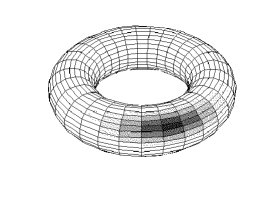
Only in the case where $n=1$ would $\Pr\left(y|\mathbf{x}\right)$ correspond to a sharply defined code cell; for $n>1$ the edges of the code cells are tapered so that they overlap with one other. The 2-torus is covered with a large number of these overlapping code cells, and when a code index $y$ is sampled from $\Pr\left(y|\mathbf{x}\right)$, it allows a reconstruction of the input to be made to within an uncertainty area commensurate with the size of a code cell. This type of encoding is called joint encoding, because the 2 intrinsic dimensions of the 2-torus are simultaneously encoded by $y$.

A typical pair of $\Pr\left(y|\mathbf{x}\right)$ (i.e. $\Pr\left(y_{1}|\mathbf{x}\right)$ and $\Pr\left(y_{2}|\mathbf{x}\right)$) for large $n$ is illustrated in figure 4.

Figure 4: Two typical probabilities $\Pr\left(y_{1}|\mathbf{x}\right)$ and $\Pr\left(y_{2}|\mathbf{x}\right)$ for encoding a 2-torus using a large value of $n$. Each separately defines a smoothly tapered collar-shaped region on the 2-torus. However, taken together, their region of intersection defines a smoothly tapered localised region on the 2-torus. The toroidal mesh serves only to help visualise the 2-torus.

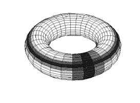
The partitioning splits the code indices into two different types: one type encodes one of the intrinsic dimensions of the 2-torus, and the other type encodes the other intrinsic dimension of the 2-torus, so each code cell is a tapered collar-shaped region. When the code indices $\left(y_{1},y_{2},\cdots,y_{n}\right)$ are sampled from $\Pr\left(y|\mathbf{x}\right)$, they allow a reconstruction of the input to be made to within an uncertainty area commensurate with the size of the region of intersection of a pair of orthogonal code cells, as illustrated in figure 4. This type of encoding is called factorial encoding, because the 2 intrinsic dimensions of the 2-torus are separately encoded in $\left(y_{1},y_{2},\cdots,y_{n}\right)$.

For a 2-torus there is an upper limit $M\approx 12$ beyond which the optimum solution is always a joint encoder (as shown in figure 3). This limit arises because when $M\gtrsim 12$ the code book is sufficiently large that the joint encoder gives the best reconstruction for all values of $n$. This result critically depends on the fact that as $n$ is increased the code cells overlap progressively more and more, so the accuracy of the reconstruction progressively increases. For $M\gtrsim 12$ the rate at which the accuracy of the joint encoder improves (as $n$ increases) is sufficiently great that it is always better than that of the factorial encoder (which also improves as $n$ increases).

2.4 Chains of Linked FMCs

Thus far it has been shown that the FMC objective function in equation 3, with the constraints imposed in equation 8, leads to useful properties, such as the automatic partitioning of the code book to yield the factorial encoder, such as that illustrated in figure 4 (and more generally, as illustrated in figure 2). The free parameters $\left(M,n\right)$ (i.e. the size of the code book, and the number of code indices sampled) can be adjusted to obtain an optimal solution that has the desired properties (e.g. a joint or a factorial encoder, as in figures 3 and 4, respectively). However, since there are only 2 free parameters, there is a limit to the variety of types of properties that the optimal solution can have. It would thus be very useful to introduce more free parameters.

The FMC illustrated in figure 1 may be generalised to a chain of linked FMCs as shown in figure 5.

Figure 5: A chain of linked FMCs, in which the output from each stage is its vector of posterior probabilities (for all values of the code index), which is then used as the input to the next stage. Only 3 stages are shown, but any number may be used. More generally, any acyclically linked network of FMCs may be used.

Each stage in this chain is an FMC of the type shown in figure 1, and the vector of probabilities (for all values of the code index) computed by each stage is used as the input vector to the next stage; there are other ways of linking the stages together, but this is the simplest possibility. The overall objective function is a weighted sum of the FMC objective functions derived from each stage. The total number of free parameters in an $L$ stage chain is $3L-1$, which is the sum of 2 free parameters for each of the $L$ stages, plus $L-1$ weighting coefficients; there are $L-1$ rather than $L$ weighting coefficients because the overall normalisation of the objective function does not affect the optimum solution.

The chain of linked FMCs may be expressed mathematically by first of all introducing an index $l$ to allow different stages of the chain to be distinguished thus

$$M \longrightarrow M^{\left(l\right)},y\longrightarrow y^{\left(l\right)}$$

$$\mathbf{x} \longrightarrow \mathbf{x}^{\left(l\right)},\mathbf{x}^{\prime}\longrightarrow\mathbf{x}^{\left(l\right)\prime}$$

$$n \longrightarrow n^{\left(l\right)},D\longrightarrow D^{\left(l\right)}$$

$$D_{1} \longrightarrow D_{1}^{\left(l\right)},D_{2}\longrightarrow D_{2}^{\left(l\right)}$$ (11)

The stages are then defined and linked together thus (the detailed are given only as far as the input to the third stage)

$$\mathbf{x}^{\left(1\right)} \longrightarrow y^{\left(1\right)}\longrightarrow\mathbf{x}^{\left(1\right)\prime}$$

$$\mathbf{x}^{\left(2\right)} = \left(x_{1}^{\left(2\right)},x_{2}^{\left(2\right)},\cdots,x_{M^{\left(1\right)}}^{\left(2\right)}\right)$$

$$x_{i}^{\left(2\right)} = \Pr\left(y^{\left(1\right)}=i|\mathbf{x}^{\left(1\right)}\right),1\leq i\leq M^{\left(1\right)}$$

$$\mathbf{x}^{\left(2\right)} \longrightarrow y^{\left(2\right)}\longrightarrow\mathbf{x}^{\left(2\right)\prime}$$

$$\mathbf{x}^{\left(3\right)} = \left(x_{1}^{\left(3\right)},x_{2}^{\left(3\right)},\cdots,x_{M^{\left(2\right)}}^{\left(3\right)}\right)$$

$$x_{i}^{\left(3\right)} = \Pr\left(y^{\left(2\right)}=i|\mathbf{x}^{\left(2\right)}\right),1\leq i\leq M^{\left(2\right)}$$ (12)

The objective function and its upper bound are then given by

$$D = \sum_{l=1}^{L}s^{\left(l\right)}D^{\left(l\right)}$$ (13)

$$\leq D_{1}+D_{2}$$

$$= \sum_{l=1}^{L}s^{\left(l\right)}\left(D_{1}^{\left(l\right)}+D_{2}^{\left(l\right)}\right)$$

where $s^{\left(l\right)}\geq 0$ is the weighting that is applied to the contribution of stage $l$ of the chain to the overall objective function.

The piecewise linearity property enjoyed by $\Pr\left(y|\mathbf{x}\right)$ in a single stage chain also holds for all of the $\Pr\left(y^{\left(l\right)}|\mathbf{x}^{\left(l\right)}\right)$ in a multi-stage chain, provided that the stages are linked together as prescribed in equation 12 [11]. This will allow optimum analytic solutions to be derived by an extension of the single stage methods used in [10].

3 Simulations

In this section the results of various numerical simulations are presented, which demonstrate some of the types of behaviour exhibited by an encoder that consists of a chain of linked FMCs. Synthetic, rather than real, training data are used in all of the simulations, because this allows the basic types of behaviour to be cleanly demonstrated.

In section 3.1 the training algorithm is presented. In section 3.2 the training data is described. In section 3.3 a single stage encoder is trained on data that is a superposition of two randomly positioned objects. In section 3.4 this is generalised to objects with correlated positions, and three different types of behaviour are demonstrated: factorial encoding using both a 1-stage and a 2-stage encoders (section 3.4.1), joint encoding using a 1-stage encoder (section 3.4.2), and invariant encoding (i.e. ignoring a subspace of the input space altogether) using a 2-stage encoder (section 3.4.3).

3.1 Training Algorithm

Assuming that $\Pr\left(y|\mathbf{x}\right)$ is modelled as in appendix A (i.e. $\Pr\left(y|\mathbf{x}\right)=\frac{Q\left(y|\mathbf{x}\right)}{\sum_{y^{\prime}=1}^{M}Q\left(y^{\prime}|\mathbf{x}\right)}$ and $Q\left(y|\mathbf{x}\right)=\frac{1}{1+\exp\left(-\mathbf{w}\left(y\right)\cdot\mathbf{x}-b\left(y\right)\right)}$), then the partial derivatives of $D_{1}+D_{2}$ with respect to the 3 types of parameters in a single stage of the encoder may be denoted as

$$\mathbf{g}_{w}\left(y\right) \equiv \frac{\partial\left(D_{1}+D_{2}\right)}{\partial\mathbf{w}\left(y\right)}$$

$$g_{b}\left(y\right) \equiv \frac{\partial\left(D_{1}+D_{2}\right)}{\partial b\left(y\right)}$$

$$\mathbf{g}_{x}\left(y\right) \equiv \frac{\partial\left(D_{1}+D_{2}\right)}{\partial\mathbf{x}^{\prime}\left(y\right)}$$ (14)

This may be generalised to each stage of a multi-stage encoder by including an $\left(l\right)$ superscript, and ensuring that for each stage the partial derivatives include the additional contributions that arise from forward propagation through later stages; this is essentially an application of the chain rule of differentiation, using the derivatives $\frac{\partial\mathbf{x}^{\left(l+1\right)}}{\partial\mathbf{w}^{\left(l\right)}\left(y^{\left(l\right)}\right)}$ and $\frac{\partial\mathbf{x}^{\left(l+1\right)}}{\partial b^{\left(l\right)}\left(y^{\left(l\right)}\right)}$ to link the stages together (see appendix A).

A simple algorithm for updating these parameters is (omitting the $\left(l\right)$ superscript, for clarity)

$$\mathbf{w}\left(y\right) \longrightarrow \mathbf{w}\left(y\right)-\varepsilon\,\frac{\mathbf{g}_{w}\left(y\right)}{g_{w,0}}$$

$$b\left(y\right) \longrightarrow b\left(y\right)-\varepsilon\,\frac{g_{b}\left(y\right)}{g_{b,0}}$$

$$\mathbf{x}^{\prime}\left(y\right) \longrightarrow \mathbf{x}^{\prime}\left(y\right)-\varepsilon\,\frac{\mathbf{g}_{x}\left(y\right)}{g_{x,0}}$$ (15)

where $\varepsilon$ is a small update step size parameter, and the three normalisation factors are defined as

$$g_{w,0} \equiv \begin{array}[]{c}\max\\ y\end{array}\sqrt{\frac{\left\|\mathbf{g}_{w}\left(y\right)\right\|^{2}}{\dim\mathbf{x}}}$$ (18)

$$g_{b,0} \equiv \begin{array}[]{c}\max\\ y\end{array}\left|b\left(y\right)\right|$$ (21)

$$g_{x,0} \equiv \begin{array}[]{c}\max\\ y\end{array}\sqrt{\frac{\left\|\mathbf{g}_{x}\left(y\right)\right\|^{2}}{\dim\mathbf{x}}}$$ (24)

The $\frac{\mathbf{g}_{w}\left(y\right)}{g_{w,0}}$ and $\frac{\mathbf{g}_{x}\left(y\right)}{g_{x,0}}$ factors ensure that the maximum update step size for $\mathbf{w}\left(y\right)$ and $\mathbf{x}^{\prime}\left(y\right)$ is $\varepsilon\dim\mathbf{x}$ (i.e. $\varepsilon$ per dimension), and the $\frac{g_{b}\left(y\right)}{g_{b,0}}$ factor ensures that the maximum update step size for $b\left(y\right)$ is $\varepsilon$. This update algorithm can be generalised to use a different $\varepsilon$ for each stage of the encoder, and also to allow a different $\varepsilon$ to be used for each of the 3 types of parameter. Furthermore, the size of $\varepsilon$ can be varied as training proceeds, usually starting with a large value, and then gradually reducing its size as the solution converges. It is not possible to give general rules for exactly how to do this, because training conditions depend very much on the statistical properties of the training set.

3.2 Training Data

The key property that this type of self-organising encoder exhibits is its ability to automatically split up high-dimensional input spaces into lower-dimensional subspaces, each of which is separately encoded. For instance, see section 2.2 for a summary of the analytically solved case of training data that lives on a simple curved manifold (i.e. a 2-torus). This self-organisation manifests itself in many different ways, depending on the interplay between the statistical properties of the training data, and the $3$ free parameters (i.e. the code book size $M$, the number of code indices sampled $n$, and the stage weighting $s$) per stage of the encoder (see section 2.4). However, it turns out that the joint and factorial encoders (of the same general type as those obtained in the case of a 2-torus) are also the optimum solutions for more general curved manifolds.

In order to demonstrate the various different basic types of self-organisation it is necessary to use synthetic training data with controlled properties. All of the types of self-organisation that will be demonstrated in this paper may be obtained by training a 1-stage or 2-stage encoder on 24-dimensional data (i.e. $M=24$) that consists of a superposition of a pair of identical objects (with circular wraparound to remove edge effects), such as is shown in figure 6.

Figure 6: An example of a typical training vector for $M=24$. Each object is a Gaussian hump with a half-width of 1.5 units, and peak amplitude of 1. The overall input vector is formed as a linear superposition of the 2 objects. Note that the input vector is wrapped around circularly to remove minor edge effects that would otherwise arise.

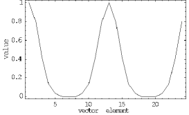
The training data is thus uniformly distributed on a manifold with 2 intrinsic circular coordinates, which is then embedded in a 24-dimensional image space. The embedding is a curved manifold, but is not a 2-torus, and there are two reasons for this. Firstly, even though the manifold has 2 intrinsic circular coordinates, the non-linear embedding distorts these circles in the 24-dimensional embedding space so that they are not planar (i.e. the profile of each object lives in the full 24-dimensional embedding space). Secondly, unlike a 2-torus, each point on the manifold maps to itself under interchange of the pair of circular coordinates, so the manifold is covered twice by a 2-torus (i.e. the objects are identical, so it makes no difference if they are swapped over). However, these differences do not destroy the general character of the joint and factorial encoder solutions that were obtained in section 2.2.

In the simulations presented below, two different methods of selecting the object positions are used: either the positions are statistically independent, or they are correlated. In the independent case, each object position is a random integer in the interval $\left[1,24\right]$. In the correlated case, the first object position is a random integer in the interval $\left[1,24\right]$, and the second object position is chosen relative to the first one as an integer in the range $\left[4,8\right]$, so that the mean object separation is $6$ units.

3.3 Independent Objects

The simplest demonstration is to let a single stage encoder discover the fact that the training data consists of a superposition of a pair of objects, which is an example of independent component analysis (ICA) or blind signal separation (BSS) [4]. This may readily be done by setting the parameters values as follows: code book size $M=16$, number of code indices sampled $n=20$, $\varepsilon=0.2$ for $250$ training steps, $\varepsilon=0.1$ for a further $250$ training steps.

The self-organisation of the $16$ reconstruction vectors as training progresses (measured down the page) is shown in figure 7.

Figure 7: A factorial encoder emerges when a single stage encoder is trained on data that is a superposition of 2 objects in independent locations.

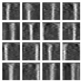
After some initial confusion, the reconstruction vectors self-organise so that each code index corresponds to a single object at a well defined location. This behaviour is non-trivial, because each training vector is a superposition of a pair of objects at independent locations, so typically more than one code index must be sampled by the encoder, which is made possible by the relatively large choice $n=20$. This result is a factorial encoder, because the objects are encoded separately. This is a rudimentary example of the type of solution that was illustrated in figure 2, although here the blocks overlap each other.

The case of a joint encoder requires a rather large code book when the objects are independent. However, when correlations between the objects are introduced then the code book can be reduced to a manageable size, as will be demonstrated in the next section.

3.4 Correlated Objects

A more interesting situation arises if the positions of the pair of objects are mutually correlated, so that the training data is non-uniformly distributed on a manifold with 2 intrinsic circular coordinates. The pair of objects can then be encoded in 3 fundamentally different ways:

1. Factorial encoder. This encoder ignores the correlations between the objects, and encodes them as if they were 2 independent objects. Each code index would thus encode a single object position, so many code indices must be sampled in order to virtually guarantee that both object positions are encoded. This result is a type of independent component analysis (ICA) [4].

2. Joint encoder. This encoder regards each possible joint placement of the 2 objects as a distinct configuration. Each code index would thus encode a pair of object positions, so only one code index needs to be sampled in order to guarantee that both object positions are encoded. This result is basically the same as what would be obtained by using a standard VQ [7].

3. Invariant encoder. This encoder regards each possible placement of the centroid of the 2 objects as a distinct configuration, but regards all possible object separations (for a given centroid) as being equivalent. Each code index would thus encode only the centroid of the pair of objects. This type of encoder does not arise when the objects are independent. This is similar to self-organising transformation invariant detectors described in [12].

Each of these 3 possibilities is shown in figure 8, where the diagrams are meant only to be illustrative. The correlated variables live in the large 2-dimensional rectangular region extending from bottom-left to top-right of each diagram. For data of the type shown in figure 6, the rectangular region is in reality the curved manifold generated by varying the pair of object coordinates, and the invariance of the data under interchange of the pair of object coodinates means that the upper left and lower right halves of each diagram cover the manifold twice.

Figure 8: Three alternative ways of using $30$ code indices to encode a pair of correlated variables. The typical code cells are shown in bold.

The factorial encoder has two orthogonal sets of long thin rectangular code cells, and the diagram shows how a pair of such cells intersect to define a small square code cell. The joint encoder behaves as a standard vector quantiser, and is illustrated as having a set of square code cells, although their shapes will not be as simple as this in practice. The invariant encoder has a set of long thin rectangular code cells that encode only the long diagonal dimension.

In all 3 cases there is overlap between code cells. In the case of the factorial and joint encoders the overlap tends to be only between nearby code cells, whereas in the case of an invariant encoder the range of the overlap is usually much greater, as will be seen in the numerical simulations below. In practice the optimum encoder may not be a clean example of one of the types illustrated in figure 8, as will also be seen in the numerical simulations below.

3.4.1 Factorial Encoding

A factorial encoder may be trained by setting the parameter values as follows: code book size $M=16$, number of code indices sampled $n=20$, $\varepsilon=0.2$ for $500$ training steps, $\varepsilon=0.1$ for a further $500$ training steps. This is the same as in the case of independent objects, except that the number of training steps has been doubled.

The result is shown in figure 9

Figure 9: A factorial encoder emerges when a single stage encoder is trained on data that is a superposition of 2 objects in correlated locations.

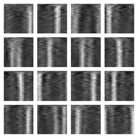
which should be compared with the result for independent objects in figure 7. The presence of correlations degrades the quality of this factorial code relative to the case of independent objects. The contamination of the factorial code takes the form of a few code indices which respond jointly to the pair of objects.

The joint coding contamination of the factorial code can be reduced by using a 2-stage encoder, in which the second stage has the same values of $M$ and $n$ as the first stage (although identical parameter values are not necessary), and (in this case) both stages have the same weighting in the objective function (see equation 13).

The results are shown in figure 10.

Figure 10: The factorial encoder is improved, by the removal of the joint encoding contamination, when a 2-stage encoder is used.

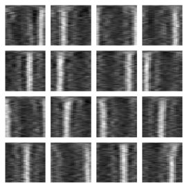
The reason that the second stage encourages the first to adopt a pure factorial code is quite subtle. The result shown in figure 10 will lead to the first stage producing an output in which 2 code indices (one for each object) typically have probability $\frac{1}{2}$ of being sampled, and all of the remaining code indices have a very small probability (this is an approximation which ignores the fact that the code cells overlap). On the other hand, figure 9 will lead to an output in which the probability is sometimes concentrated on a single code index. However, the contribution of the second stage to the overall objective function encourages it to encode the vector of probabilities output by the first stage with minimum Euclidean reconstruction error, which is easier to do if the situation is as in figure 10 rather than as in figure 9. In effect, the second stage likes to see an output from the first stage in which a large number of code indices are each sampled with a low probability, which favours factorial coding over joint encoding.

3.4.2 Joint Encoding

A joint encoder may be trained by setting the parameter values as follows: code book size $M=16$, number of code indices sampled $n=3$, $\varepsilon=0.2$ for $500$ training steps, $\varepsilon=0.1$ for a further $500$ training steps, $\varepsilon=0.05$ for a further $1000$ training steps. This is the same as the parameter values for the factorial encoder above, except that $n$ has been reduced to $n=3$, and the training schedule has been extended.

The result is shown in figure 11.

Figure 11: A joint encoder emerges when a single stage encoder is trained on data that is a superposition of 2 objects in correlated locations.

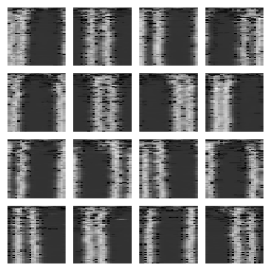
After some initial confusion, the reconstruction vectors self-organise so that each code index corresponds to a pair of objects at well defined locations, so the code index jointly encodes the pair of object positions; this is a joint encoder. The small value of $n$ prevents a factorial encoder from emerging.

3.4.3 Invariant Encoding

An invariant encoder may be trained by using a 2-stage encoder, and setting the parameter values identically in each stage as follows (where the weighting of the second stage relative to the first is denoted as $s$): code book size $M=16$, number of code indices sampled $n=3$, $\varepsilon=0.2$ and $s=5$ for $500$ training steps, $\varepsilon=0.1$ and $s=10$ for a further $500$ training steps, $\varepsilon=0.05$ and $s=20$ for a further $500$ training steps, $\varepsilon=0.05$ and $s=40$ for a further $500$ training steps. This is basically the same as the parameter values used for the joint encoder above, except that there are now 2 stages, and the weighting of the second stage is progressively increased throughout the training schedule. Note that the large value that is used for $s$ is offset to a certain extent by the fact that the ratio of the normalisation of the inputs to the first and second stages is very large; the anomalous normalisation of the input to the first stage could be removed by insisting that the input to the first stage is a vector of probabilities, but that is not done in these simulations.

The result is shown in figure 12.

Figure 12: An invariant encoder emerges when 2-stage encoder is trained on data that is a superposition of 2 objects in correlated locations.

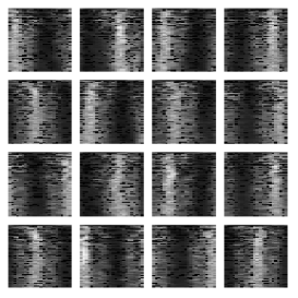
During the early part of the training schedule the weighting of the second stage is still relatively small, so it has the effect of turning what would otherwise have been a joint encoder into a factorial encoder; this is analogous to the effect observed when figure 9 becomes figure 10. However, as the training schedule progresses the weighting of the second stage increases further, and the reconstruction vectors self-organise so that each code index corresponds to a pair of objects with a well defined centroid but indeterminate separation. Thus each code index encodes only the centroid of the pair of objects and ignores their separation. This is a new type of encoder that arises when the objects are correlated, and it will be called an invariant encoder, in recognition of the fact that its output is invariant with respect to the separation of the objects.

Note that in these results there is a large amount of overlap between the code cells, which should be taken into account when interpreting the illustration in figure 8.

4 Conclusions

The numerical results presented in this paper show that a stochastic vector quantiser (VQ) can be trained to find a variety of different types of way of encoding high-dimensional input vectors. These input vectors are generated in two stages. Firstly, a low-dimensional manifold is created whose intrinsic coordinates are the positions of the objects in the scene; this corresponds to generating the scene itself. Secondly, this manifold is non-linearly embedded to create a curved manifold that lives in a high-dimensional space of image pixel values; this corresponds to imaging the generated scene.

Three fundamentally different types of encoder have been demonstrated, which differ in the way that they build a reconstruction that approximates the input vector:

1. A factorial encoder uses a reconstruction that is superposition of a number of vectors that each lives in a well defined input subspace, which is useful for discovering constituent objects in the input vector. This result is a type of independent component analysis (ICA) [4].

2. A joint encoder uses a reconstruction that is a single vector that lives in the whole input space. This result is basically the same as what would be obtained by using a standard VQ [7].

3. An invariant encoder uses a reconstruction that is a single vector that lives in a subspace of the whole input space, so it ignores some dimensions of the input vector, which is therefore useful for discovering correlated objects whilst rejecting uninteresting fluctuations in their relative coordinates. This is similar to self-organising transformation invariant detectors described in [12].

More generally, the encoder will be a hybrid of these basic types, depending on the interplay between the statistical properties of the input vector and the parameter settings of the SVQ.

5 Acknowledgement

I thank Chris Webber for many useful conversations that we had during the course of this research.

Appendix A Derivatives of the Objective Function

In order to minimise $D_{1}+D_{2}$ it is necessary to compute its derivatives. The derivatives were presented in detail in [9] for a single stage chain (i.e. a single FMC). The purpose of this appendix is to extend this derivation to a multi-stage chain of linked FMCs. In order to write the various expressions compactly, infinitesimal variations will be used thoughout this appendix, so that $\delta\left(uv\right)=\delta u\,\,v+u\,\delta v$ will be written rather than $\frac{\partial\left(uv\right)}{\partial\theta}=\frac{\partial u}{\partial\theta}\,v+u\,\frac{\partial v}{\partial\theta}$ (for some parameter $\theta$). The calculation will be done in a top-down fashion, differentiating the objective function first, then differentiating anything that the objective function depends on, and so on following the dependencies down until only constants are left (this is essentially the chain rule of differentiation).

The derivative of $D_{1}+D_{2}$ (defined in equation 13) is given by

$$\delta\sum_{l=1}^{L}s^{\left(l\right)}\left(D_{1}^{\left(l\right)}+D_{2}^{\left(l\right)}\right)=\sum_{l=1}^{L}s^{\left(l\right)}\left(\delta D_{1}^{\left(l\right)}+\delta D_{2}^{\left(l\right)}\right)$$ (25)

The derivatives of the $D_{1}^{\left(l\right)}$ and $D_{2}^{\left(l\right)}$ parts (defined in equation 10, with appropriate $\left(l\right)$ superscripts added) of the contribution of stage $l$ to $D_{1}+D_{2}$ are given by (dropping the $\left(l\right)$ superscripts again, for clarity)

$$\delta D_{1} = \frac{2}{n}\int d\mathbf{x}\Pr\left(\mathbf{x}\right)\sum_{y=1}^{M}\left(\begin{array}[]{c}\delta\Pr\left(y|\mathbf{x}\right)\left\|\mathbf{x}-\mathbf{x}^{\prime}\left(y\right)\right\|^{2}\\ +2\Pr\left(y|\mathbf{x}\right)\left(\delta\mathbf{x-}\delta\mathbf{x}^{\prime}\left(y\right)\right)\cdot\left(\mathbf{x}-\mathbf{x}^{\prime}\left(y\right)\right)\end{array}\right)$$ (28)

$$\delta D_{2} = \frac{4\left(n-1\right)}{n}\int d\mathbf{x}\Pr\left(\mathbf{x}\right)\sum_{y=1}^{M}\left[\begin{array}[]{c}\left(\begin{array}[]{c}\delta\mathbf{x}\\ -\sum_{y^{\prime}=1}^{M}\left(\begin{array}[]{c}\delta\Pr\left(y^{\prime}|\mathbf{x}\right)\mathbf{x}^{\prime}\left(y^{\prime}\right)\\ +\Pr\left(y^{\prime}|\mathbf{x}\right)\delta\mathbf{x}^{\prime}\left(y^{\prime}\right)\end{array}\right)\end{array}\right)\\ \cdot\left(\mathbf{x}-\sum_{y^{\prime}=1}^{M}\Pr\left(y^{\prime}|\mathbf{x}\right)\mathbf{x}^{\prime}\left(y^{\prime}\right)\right)\end{array}\right]$$ (35)

In numerical simulations the exact piecewise linear solution for the optimum $\Pr\left(y|\mathbf{x}\right)$ (see section 2.3) will not be sought, rather $\Pr\left(y|\mathbf{x}\right)$ will be modelled using a simple parametric form, and then the parameters will be optimised. This model of $\Pr\left(y|\mathbf{x}\right)$ will not in general include the ideal piecewise linear optimum solution, so using it amounts to replacing $D_{1}+D_{2}$, which is an upper bound on the objective function $D$ (see equation 13), by an even weaker upper bound on $D$. The justification for using this approach rests on the quality of the results that are obtained from the resulting numerical simulations (see section 3).

The first step in modelling $\Pr\left(y|\mathbf{x}\right)$ is to explicitly state the fact that it is a probability, which is a normalised quantity. This may be done as follows

$$\Pr\left(y|\mathbf{x}\right)=\frac{Q\left(y|\mathbf{x}\right)}{\sum_{y^{\prime}=1}^{M}Q\left(y^{\prime}|\mathbf{x}\right)}$$ (36)

where $Q\left(y|\mathbf{x}\right)\geq 0$ (note that there is a slight change of notation compared with [9], because $Q\left(y|\mathbf{x}\right)$ rather than $Q\left(\mathbf{x}|y\right)$ is written, but the results are equivalent). The $Q\left(y|\mathbf{x}\right)$ are thus unnormalised probabilities, and $\sum_{y^{\prime}=1}^{M}Q\left(y^{\prime}|\mathbf{x}\right)$ is the normalisation factor. The derivative of $\Pr\left(y|\mathbf{x}\right)$ is given by

$$\frac{\delta\Pr\left(y|\mathbf{x}\right)}{\Pr\left(y|\mathbf{x}\right)}=\frac{1}{Q\left(y|\mathbf{x}\right)}\left(\delta Q\left(y|\mathbf{x}\right)-\Pr\left(y|\mathbf{x}\right)\sum_{y^{\prime}=1}^{M}\delta Q\left(y^{\prime}|\mathbf{x}\right)\right)$$ (37)

The second step in modelling $\Pr\left(y|\mathbf{x}\right)$ is to introduce an explicit parameteric form for $Q\left(y|\mathbf{x}\right)$. The following sigmoidal function will be used in this paper

$$Q\left(y|\mathbf{x}\right)=\frac{1}{1+\exp\left(-\mathbf{w}\left(y\right)\cdot\mathbf{x}-b\left(y\right)\right)}$$ (38)

where $\mathbf{w}\left(y\right)$ is a weight vector and $b\left(y\right)$ is a bias. The derivative of $Q\left(y|\mathbf{x}\right)$ is given by

$$\delta Q\left(y|\mathbf{x}\right)=Q\left(y|\mathbf{x}\right)\left(1-Q\left(y|\mathbf{x}\right)\right)\left(\delta\mathbf{w}\left(y\right)\cdot\mathbf{x+w}\left(y\right)\cdot\delta\mathbf{x}+\delta b\left(y\right)\right)$$ (39)

There are also $\delta\mathbf{x}$ derivatives in equation 35 and equation 39. The $\delta\mathbf{x}$ derivative arises only in multi-stage chains of FMCs, and because of the way in which stages of the chain are linked together (see equation 12) it is equal to the derivative of the vector of probabilities output by the previous stage. Thus the $\delta\mathbf{x}$ derivative may be obtained by following its dependencies back through the stages of the chain until the first layer is reached; this is essentially the chain rule of differentiation. This ensures that for each stage the partial derivatives include the additional contributions that arise from forward propagation through later stages, as described in section 3.1.

There are also $\delta\mathbf{x}^{\prime}\left(y\right)$ derivatives in equation 35, but these require no further simplification.

References

- [1] Farvardin N, 1990, A study of vector quantisation for noisy channels, IEEE Transactions on Information Theory, 36, 799-809.
- [2] Gersho A and Gray R M, 1992, Vector quantisation and signal processing, Kluwer.
- [3] Gray R M, 1984, Vector quantisation, IEEE Acoust., Speech, Signal Processing Mag., April 1984, 4-29.
- [4] Hyvärinen A, 1999, Survey on independent component analysis, Neural Computing Surveys, 2, 94-128.
- [5] Kohonen T, 1984, Self-organisation and associative memory, Springer-Verlag.
- [6] Kumazawa H, Kasahara M and Namekawa T, 1984, A construction of vector quantisers for noisy channels, Electronic Engineering Japan, 67B, 39-47.
- [7] Linde Y, Buzo A and Gray R M, 1980, An algorithm for vector quantiser design, IEEE Trans. COM, 28, 84-95.
- [8] Luttrell S P, 1994, A Bayesian analysis of self-organising maps, Neural Computation, 6, 767-794.
- [9] Luttrell S P, 1997, A theory of self-organising neural networks, in Mathematics of Neural Networks: Models, Algorithms and Applications, Kluwer, Ellacott S W, Mason J C and Anderson I J (eds.), 240-244.
- [10] Luttrell S P, 1999, Self-organised modular neural networks for encoding data, in Combining Artificial Neural Nets: Ensemble and Modular Multi-Net Systems, 235-263, Springer-Verlag, Sharkey A J C (ed.).
- [11] Luttrell S P, 1999, An adaptive network for encoding data using piecewise linear functions, to appear in Proceedings of the 9th International Conference on Artificial Neural Networks (ICANN99), Edinburgh, 7-10 September 1999.
- [12] Webber C J S, 1994, Self-organisation of transformation-invariant detectors for constituents of perceptual patterns, Network: Computation in Neural Systems, 5, 471-496.
- [13] Yair E, Zeger K and Gersho A, 1992, Competitive learning and soft competition for vector quantiser design, IEEE Transactions on Signal Processing, 40, 294-309.