Decoherence in Quantum Mechanics

Abstract

We study decoherence in a simple quantum mechanical model using two approaches. Firstly, we follow the conventional approach to decoherence where one is interested in solving the reduced density matrix from the perturbative master equation. Secondly, we consider our novel correlator approach to decoherence where entropy is generated by neglecting observationally inaccessible correlators. We show that both methods can accurately predict decoherence time scales. However, the perturbative master equation generically suffers from instabilities which prevents us to reliably calculate the system’s total entropy increase. We also discuss the relevance of the results in our quantum mechanical model for interacting field theories.

I Introduction

I.1 The Correlator Approach to Decoherence

Recently, we proposed a novel approach to decoherence based on neglecting observationally inaccessible correlators Koksma:2009wa ; Koksma:2010zi , also see Giraud:2009tn . Just as in the conventional approach to decoherence Zeh:1970 ; Zurek:1981xq ; Joos:1984uk ; Zurek:1991vd , we split our world into a distinct system, environment, and observer. Interactions between system and environment in quantum field theory generate non-Gaussian correlators. However, from the observer’s perspective, these correlators are generically small in the perturbative sense. The observer’s inability to measure the information stored in these higher order correlators generates a certain amount of entropy which turns our quantum system into a classical stochastic system. We applied our “correlator approach” to decoherence to an interacting quantum field theoretical model Koksma:2009wa , with an interaction term of the form $h\phi(x)\chi^{2}(x)$, by solving for the renormalised statistical propagator in an out-of-equilibrium setting. Giraud and Serreau Giraud:2009tn performed a similar analysis in a $\lambda\phi^{4}(x)$ field theory. Starting point is the well known von Neumann entropy:

$$S_{\rm vN}=-{\rm Tr}[\hat{\rho}\ln(\hat{\rho})]\,,$$ (1)

where $\hat{\rho}$ denotes the density operator which in the Schrödinger picture satisfies the von Neumann equation:

$$\imath\hbar\frac{\partial}{\partial t}\hat{\rho}=[\hat{H},\hat{\rho}]\,.$$ (2)

By restricting ourselves to a Gaussian density matrix (and thus neglecting all non-Gaussian information that is contained in the full density matrix), one can easily relate the Gaussian von Neumann entropy to the statistical propagator of our field theoretical system Koksma:2010zi ; Campo:2008ij . This procedure can be improved by including non-Gaussian corrections to the entropy Koksma:2010zi . Indeed, the Gaussian von Neumann entropy is in most cases no longer conserved, unlike the total von Neumann entropy in equation (1).

We thus argue to solve directly for the Gaussian correlators characterising the Gaussian properties of our system. A sophisticated field theoretical framework exists to renormalise the statistical propagator, include perturbative corrections and study genuine time evolution in an out-of-equilibrium setting (see e.g. Berges:2004yj ; Garny:2009ni ).

I.2 The Master Equation Approach to Decoherence and its Shortcomings

In the conventional approach to decoherence one is interested in solving for the reduced density matrix which is obtained by tracing over the environmental degrees of freedom in the full density matrix:

$$\hat{\rho}_{\mathrm{red}}(t)=\mathrm{Tr}_{E}[\hat{\rho}(t)]\,.$$ (3)

The unitary von Neumann equation (2) transforms to a non-unitary master equation for $\hat{\rho}_{\mathrm{red}}$. The master equation is in principle equivalent to the von Neumann equation if no approximations are made. This is for example clear from the influence functional method. In other words: the exact master equation is just as hard to solve as the von Neumann equation in interacting quantum field theories. Therefore, one usually relies on perturbative methods to simplify the exact master equation and to derive a perturbative master equation.

The conventional approach to decoherence suffers from both theoretical and practical shortcomings. From a theoretical point of view, it is disturbing that $\rho_{\mathrm{red}}$ is obtained from a non-unitary equation despite of the fact that the underlying theory is unitary. Practically speaking, the (exact or perturbative) master equation is still so hard to solve that even the most basic field theoretical questions have never been properly addressed: no well established framework exists to include perturbative corrections to a reduced density matrix (see however the pioneering work in quantum mechanical cases Hu:1993vs ; Hu:1993qa ; Calzetta:book ) nor has any reduced density matrix ever been renormalised.

I.3 A Clean Comparison Between the Two Approaches

As a solution to the perturbative master equation in a field theoretical setting has so far not been derived, let us study a simple quantum mechanical model. Quantum mechanics thus provides us with the ideal playing field to compare the two approaches to decoherence. In this paper we study a well known textbook example Grabert:1988yt ; Paz:2000le ; Zurek:2003zz ; Calzetta:book of $N+1$ simple harmonic oscillators. Here, one oscillator, $x$, plays the role of the system and the other $N$ oscillators, $q_{n}$, $1\leq n\leq N$, play the role of the environment. The oscillators will be coupled quadratically: $\lambda_{n}xq_{n}$. In quantum mechanics we do not have to worry about divergences and moreover, since we have chosen our model to be Gaussian, we can actually compute the reduced density matrix by tracing over the environmental degrees of freedom. Indeed, all the practical shortcomings to the conventional approach to decoherence as listed above have thus been circumvented.

Furthermore, it is important to realise that the entropy in our correlator approach to decoherence is not generated by neglecting non-Gaussianities as our quantum mechanical model is Gaussian. Instead, the correlation entropy between the system and environment that builds up due to the coupling between the two is neglected. The correlation entropy in this paper thus plays the role of the non-Gaussian contributions to the entropy in a proper field theory. In this paper we present two calculations:

• We calculate the evolution of the entropy by solving for the reduced density matrix from the perturbative master equation;

• We calculate the evolution of the entropy by solving for the Gaussian correlators directly from which we calculate the Gaussian von Neumann entropy.

In particular we identify regions in parameter space where the perturbative master equation performs well and where it does not. In section II we introduce the model and in section III we outline two derivations of the perturbative master equation. In sections IV and V we analyse the evolution of the entropy for $N=1$ and $N=50$, respectively.

II The Model

II.1 Bilinearly Coupled Simple Harmonic Oscillators

We consider the following total quantum mechanical action:

$$S\left[\tilde{x},\{\tilde{q}_{n}\}\right]=\int\mathrm{d}tL\left[\tilde{x},\{\tilde{q}_{n}\}\right]=\int\mathrm{d}t\left\{L_{\mathrm{S}}\left[\tilde{x}\right]+L_{\mathrm{E}}\left[\{\tilde{q}_{n}\}\right]+L_{\mathrm{Int}}\left[\tilde{x},\{\tilde{q}_{n}\}\right]\right\}\,,$$ (4)

where:

$$L_{\mathrm{S}}\left[\tilde{x}\right] = \frac{1}{2}m\dot{\tilde{x}}^{2}-\frac{1}{2}m\omega^{2}_{0}\tilde{x}^{2}$$ (5a)

$$L_{\mathrm{E}}\left[\{\tilde{q}_{n}\}\right] = \sum_{n=1}^{N}\left(\frac{1}{2}m_{n}\dot{\tilde{q}}_{n}^{2}-\frac{1}{2}m_{n}\omega_{n}^{2}\tilde{q}_{n}^{2}\right)$$ (5b)

$$L_{\mathrm{Int}}\left[\tilde{x},\{\tilde{q}_{n}\}\right] = -\sum_{n=1}^{N}\tilde{\lambda}_{n}\tilde{q}_{n}\tilde{x}\,.$$ (5c)

Here $\tilde{x}=\tilde{x}(t)$ denotes the system coordinate and $\tilde{q}_{n}=\tilde{q}_{n}(t)$ with $n=1,\cdots,N$ are the environment coordinates. It is useful to perform the rescaling:

$$x = \sqrt{m}\tilde{x}$$ (6a)

$$q_{n} = \sqrt{m_{n}}\tilde{q}_{n}\,,$$ (6b)

after which the Lagrangian in equation (4) becomes:

$$L\big{[}x,\{q_{n}\}\big{]}=\frac{1}{2}{\dot{x}}^{2}-\frac{1}{2}\omega^{2}_{0}x^{2}+\sum_{n=1}^{N}\left(\frac{1}{2}{\dot{q}}_{n}^{2}-\frac{1}{2}\omega_{n}^{2}q_{n}^{2}\right)-\sum_{n=1}^{N}\lambda_{n}q_{n}x\,,$$ (7)

where $\lambda_{n}=\tilde{\lambda}_{n}/\sqrt{mm_{n}}$. Throughout the paper we will set $\langle\hat{x}\rangle=0$ and $\langle\hat{q}_{n}\rangle=0$, $1\leq n\leq N$. In order to understand how to impose initial conditions later on, it is useful to explicitly derive the statistical propagator in thermal equilibrium. In thermal equilibrium the Schwinger-Keldysh propagators for e.g. the coordinate $x$ are given by:

$$\imath\Delta^{++}(t;t^{\prime}) = \frac{\cos(\omega_{0}\Delta t)}{2\omega_{0}}\coth\Big{(}\frac{\beta\omega_{0}}{2}\Big{)}-\frac{\imath}{2}{\rm sign}(\Delta t)\frac{\sin(\omega_{0}\Delta t)}{\omega_{0}}$$ (8a)

$$\imath\Delta^{--}(t;t^{\prime}) = \frac{\cos(\omega_{0}\Delta t)}{2\omega_{0}}\coth\Big{(}\frac{\beta\omega_{0}}{2}\Big{)}+\frac{\imath}{2}{\rm sign}(\Delta t)\frac{\sin(\omega_{0}\Delta t)}{\omega_{0}}=\Big{[}\imath\Delta^{--}(t;t^{\prime})\Big{]}^{*}$$ (8b)

$$\imath\Delta^{+-}(t;t^{\prime}) = \frac{\cos(\omega_{0}\Delta t)}{2\omega_{0}}\coth\Big{(}\frac{\beta\omega_{0}}{2}\Big{)}+\frac{\imath}{2}\frac{\sin(\omega_{0}\Delta t)}{\omega_{0}}$$ (8c)

$$\imath\Delta^{-+}(t;t^{\prime}) = \frac{\cos(\omega_{0}\Delta t)}{2\omega_{0}}\coth\Big{(}\frac{\beta\omega_{0}}{2}\Big{)}-\frac{\imath}{2}\frac{\sin(\omega_{0}\Delta t)}{\omega_{0}}=\Big{[}\imath\Delta^{+-}(t;t^{\prime})\Big{]}^{*}\,,$$ (8d)

where $\beta=1/(k_{B}T)$, with $k_{B}$ the Stefan-Boltzmann constant and where we defined $\Delta t=t-t^{\prime}$. The causal and statistical propagators now follow as the sum and the difference of the two Wightman propagators:

$$\Delta^{c}(t;t^{\prime}) = \Delta^{-+}(t;t^{\prime})-\Delta^{+-}(t;t^{\prime})=-\frac{\sin(\omega_{0}\Delta t)}{\omega_{0}}$$ (9a)

$$F(t;t^{\prime}) = \frac{1}{2}\Big{(}\imath\Delta^{-+}(t;t^{\prime})+\imath\Delta^{+-}(t;t^{\prime})\Big{)}=\frac{\cos(\omega_{0}\Delta t)}{2\omega_{0}}\coth\Big{(}\frac{\beta\omega_{0}}{2}\Big{)}\,.$$ (9b)

II.2 The Von Neumann Entropy in Quantum Mechanics

II.2.1 $\lambda=0$

It is important to realise that since the Lagrangian in equation (7) is Gaussian, no non-Gaussianities are generated by the coupling $\lambda$. For a free quantum mechanical system ($\lambda=0$), it is simple to find the total von Neumann entropy in equation (1):

$$S_{\mathrm{vN}}=-\mathrm{Tr}[\hat{\rho}_{\mathrm{f}}\log\hat{\rho}_{\mathrm{f}}]\,,$$

where the subscript “f” for “free” reminds us that all interactions or couplings are switched off. The density operator of a quantum mechanical Gaussian state centered at the origin is of the form:

$$\hat{\rho}_{\mathrm{f}}(t)=\int_{-\infty}^{\infty}\mathrm{d}x\int_{-\infty}^{\infty}\mathrm{d}y|x\rangle\rho_{\mathrm{f}}(x,y;t)\langle y|\,,$$ (10a)

where:

$$\rho_{\mathrm{f}}(x,y;t)={\cal N}(t)\exp\left[-a(t)x^{2}-b(t)y^{2}+2c(t)xy\right]\,,$$ (10b)

and where $a=a(t)$, $b=b(t)$ and $c=c(t)$ are determined from the von Neumann equation. Moreover, from $\hat{\rho}_{\mathrm{f}}^{\dagger}=\hat{\rho}_{\mathrm{f}}$ it follows that $b^{*}=a$ and $c^{*}=c$. When $c\neq 0$ the density matrix is mixed and entangled. The normalisation ${\cal N}$ is obtained from requiring $\mathrm{Tr}[\hat{\rho}_{\mathrm{f}}]=1$:

$${\cal N}=\sqrt{\frac{2(a_{\mathrm{R}}-c)}{\pi}}\,,$$ (11)

provided that $c<a_{\mathrm{R}}$ where $a_{\mathrm{R}}=\Re[a]$. We can furthermore derive the three non-trivial Gaussian correlators characterising our system:

$$\langle\hat{x}^{2}\rangle = {\rm Tr}[\hat{\rho}_{\mathrm{f}}\hat{x}^{2}]=\int_{-\infty}^{\infty}\mathrm{d}\tilde{x}\langle\tilde{x}|\hat{\rho}_{\mathrm{f}}\hat{x}^{2}|\tilde{x}\rangle=\frac{1}{4(a_{\mathrm{R}}-c)}$$ (12a)

$$\Big{\langle}\frac{1}{2}\{\hat{x},\hat{p}\}\Big{\rangle} = -\frac{a_{\mathrm{I}}}{2(a_{\mathrm{R}}-c)}$$ (12b)

$$\langle\hat{p}^{2}\rangle = \frac{|a|^{2}-c^{2}}{a_{\mathrm{R}}-c}\,.$$ (12c)

We used $\langle x|\hat{p}|\psi\rangle=-\imath\partial_{x}\langle x|\psi\rangle$. These relations can be inverted:

$$a_{\mathrm{I}} = -\frac{\left\langle\frac{1}{2}\{\hat{x},\hat{p}\}\right\rangle}{2\langle\hat{x}^{2}\rangle}$$ (13a)

$$a_{\mathrm{R}} = \frac{\Delta^{2}+1}{8\langle\hat{x}^{2}\rangle}$$ (13b)

$$c = \frac{\Delta^{2}-1}{8\langle\hat{x}^{2}\rangle}\,,$$ (13c)

We can straightforwardly find the von Neumann entropy by making use of the replica trick (see e.g. Koksma:2010zi ):

$$S_{\rm vN}=\frac{\Delta+1}{2}\ln\left(\frac{\Delta+1}{2}\right)-\frac{\Delta-1}{2}\ln\left(\frac{\Delta-1}{2}\right)\,,$$ (14)

where:

$$\Delta^{2}=\frac{a_{\mathrm{R}}+c}{a_{\mathrm{R}}-c}=4\left[\langle\hat{x}^{2}\rangle\langle\hat{p}^{2}\rangle-\Big{\langle}\frac{1}{2}\{\hat{x},\hat{p}\}\Big{\rangle}^{2}\right]=4\left.\left[F(t;t^{\prime})\partial_{t}\partial_{t^{\prime}}F(t;t^{\prime})-\{\partial_{t}F(t;t^{\prime})\}^{2}\right]\right|_{t=t^{\prime}}\,.$$ (15)

The physical meaning of $\Delta/2$ is the phase space area occupied by a Gaussian state centered at the origin in units of $\hbar$. For a pure state we have $\Delta=1$, whereas for a mixed state $\Delta>1$. The phase space area is an extremely important function, as it coincides precisely with the area the state occupies in Wigner space Koksma:2010zi and is moreover conserved by the evolution $\mathrm{d}/\mathrm{d}t[\Delta^{2}]=0$ in free theories. It is also important to mention that we can associate a statistical particle number to $\Delta$ given by $n=(\Delta-1)/2$ such that the von Neumann entropy reduces to the well-known entropy of $n$ free Bose particles per quantum state.

II.2.2 $\lambda\neq 0$

As in all unitary systems, the von Neumann entropy following from equation (1) is conserved:

$$S_{\mathrm{vN}}=\mathrm{const}\,.$$ (16)

The von Neumann entropy for the model (7) contains both information about the system, the environment and the correlations between system and environment that are generated due to the coupling:

$$S_{\mathrm{vN}}=S_{\mathrm{total}}=S_{S}(t)+S_{E}(t)+S_{SE}(t)\,.$$ (17)

where $S_{S}$ and $S_{E}$ represent the Gaussian von Neumann entropy contained in the system and environment separately, and where $S_{SE}$ denotes the Gaussian correlation entropy. Adding the word “Gaussian” to these entropies might at the moment seem redundant, because our total system and environment are Gaussian so no non-Gaussianities can be generated as we mentioned before. We nevertheless insist on this nomenclature in order to easily compare it with interacting field theories later. For a free system $S$ that is not coupled to or in interaction with an environment $E$ we have derived the von Neumann entropy in equation (14) and (15). Likewise, we can associate a Gaussian von Neumann entropy to our system $S$ in the presence of a coupling $\lambda$ too:

$$S_{S}(t)=\frac{\Delta(t)+1}{2}\ln\left(\frac{\Delta(t)+1}{2}\right)-\frac{\Delta(t)-1}{2}\ln\left(\frac{\Delta(t)-1}{2}\right)\,,$$ (18)

where the phase space area is given in equation (15) and follows from measuring the three non-trivial equal time Gaussian correlators characterising the properties of the system: $\langle\hat{x}^{2}\rangle$, $\langle\hat{p}_{x}^{2}\rangle$ and $1/2\langle\{\hat{x},\hat{p}_{x}\}\rangle$. Note that for the coupled system $S_{S}(t)$ is generally not conserved. A similar argument applies to the environmental oscillators and we can likewise associate an environmental entropy to all $q_{n}$ if we measure its properties. Since the total von Neumann entropy is conserved in equation (17), we can then find the time evolution of the correlation entropy by solving:

$$S_{SE}(t)=S_{\mathrm{vN}}-S_{S}(t)-S_{E}(t)=S_{S}(0)+S_{E}(0)-S_{S}(t)-S_{E}(t)\,,$$ (19)

where we assumed that $S_{SE}(0)=0$ initially. What we would refer to as “Gaussian von Neumann entropy” is referred to as “correlation entropy” in Calzetta:2003dk , where they prove an $H$-theorem for a quantum mechanical $O(N)$ model.

The reduced density matrix captures the average effect from the environmental oscillators on our system oscillator and is defined in equation (3):

$$\hat{\rho}_{\mathrm{red}}(t)=\mathrm{Tr}_{E}[\hat{\rho}(t)]\,.$$

In order to quantify the amount of decoherence that has taken place, one is interested in the “reduced von Neumann entropy” which we can define by:

$$S_{\mathrm{vN}}^{\mathrm{red}}(t)=-\mathrm{Tr}[\hat{\rho}_{\mathrm{red}}(t)\log\hat{\rho}_{\mathrm{red}}(t)]\,.$$ (20)

The Gaussian von Neumann entropy we defined in equation (18) is identical to the “reduced von Neumann entropy” defined above:

$$S_{S}(t)=S_{\mathrm{vN}}^{\mathrm{red}}(t)\,.$$ (21)

The argument is trivial:

$$\langle\hat{x}^{2}\rangle={\rm Tr}[\hat{\rho}\hat{x}^{2}]=\int_{-\infty}^{\infty}\mathrm{d}\tilde{x}\mathrm{d}\tilde{q}\langle\tilde{x}\tilde{q}|\hat{\rho}\hat{x}^{2}|\tilde{q}\tilde{x}\rangle={\rm Tr}_{S}[\hat{\rho}_{\mathrm{red}}\hat{x}^{2}]\,,$$ (22)

and similar expressions hold for $\langle\{\hat{x},\hat{p}_{x}\}\rangle$ and $\langle\hat{p}_{x}^{2}\rangle$. Since the value of all three non-trivial Gaussian correlators does not depend on whether we evaluate the expectation value with the full density matrix or with the reduced density matrix, the value of the phase space area $\Delta(t)$ or indeed the entropy is identical in both cases. We show this explicitly using our coupled system of simple harmonic oscillators in appendix B. Of course, when proper (non-Gaussian) interactions are considered, equation (21) is only true for the “Gaussian reduced von Neumann entropy” $S_{\mathrm{vN}}^{\mathrm{G,red}}(t)$ based on including Gaussian correlators only.

III The Master Equation

In this section we outline for completeness two derivations of the master equation. Paz and Zurek nicely derive the master equation by means of perturbative methods Paz:2000le before they review the “influence functional method”. The latter was pioneered by Caldeira and Leggett Caldeira:1982iu , see also the early review of Grabert, Schramm and Ingold Grabert:1988yt , which in principle allows us to derive a non-perturbative master equation Su:1987pi ; Hu:1991di ; Hu:1993vs ; Hu:1993qa ; Chou:2007jg . In the perturbative approximation both derivations yield the same master equation.

One defines the reduced density matrix by tracing over the environmental degrees of freedom in the full density matrix as in equation (3). In most of the cases of physical interest, it is impossible to solve for the von Neumann equation of the density matrix exactly. Hence, it is impossible to perform the trace to find the reduced density matrix exactly. Consequently, in order to write down an equation of motion for $\rho_{\mathrm{red}}$ that is usually referred to as a “master equation”, one makes certain approximations to the von Neumann equation. For example, one can make a perturbative approximation or neglect the backreaction from the system on the environment. The master equation is non-unitary in nature which is precisely what generates the entropy.

Let us state again explicitly at this point that there is nothing wrong with tracing over environmental degrees of freedom per se, it is the perturbative master equation that is used to obtain the “reduced density matrix” that fails to capture the correct physics at late times as we will see later.

Let us begin by following the perturbative approach as outlined by Paz and Zurek in e.g. Paz:2000le . The Hamiltonian following from (7) is given by:

$$\hat{H}=\hat{H}_{S}+\hat{H}_{E}+\hat{H}_{\mathrm{Int}}=\frac{1}{2}\hat{p}_{x}^{2}+\frac{1}{2}\omega^{2}_{0}\hat{x}^{2}+\sum_{n=1}^{N}\left(\frac{1}{2}\hat{p}_{q_{n}}^{2}+\frac{1}{2}\omega_{n}^{2}\hat{q}_{n}^{2}+\lambda_{n}\hat{q}_{n}\hat{x}\right)\,.$$ (23)

The perturbative solution to the von Neumann equation (2) is the Dyson series which is truncated at second order. We can now trace over the environmental degrees of freedom to obtain:

$$\dot{\hat{\rho}}_{\mathrm{red}}^{\mathrm{I}}(t)=\frac{1}{i\hbar}\mathrm{Tr}_{E}[\hat{H}_{\mathrm{Int}}^{\mathrm{I}}(t),\hat{\rho}(0)]-\frac{1}{\hbar^{2}}\int_{0}^{t}\mathrm{d}t_{1}\mathrm{Tr}_{E}[\hat{H}_{\mathrm{Int}}^{\mathrm{I}}(t),[\hat{H}_{\mathrm{Int}}^{\mathrm{I}}(t_{1}),\hat{\rho}(0)]]\,.$$ (24)

Here, the superscript $\mathrm{I}$ denotes the interaction picture such that $\hat{H}_{\mathrm{Int}}^{\mathrm{I}}(t)=\hat{U}_{0}^{{\dagger}}\hat{H}_{\mathrm{Int}}(0)\hat{U}_{0}$, with $\hat{U}_{0}=\exp[-i/\hbar(\hat{H}_{S}+\hat{H}_{E})]$. If one now assumes that initially the total density matrix is not entangled, i.e.: $\hat{\rho}(0)=\hat{\rho}_{S}(0)\otimes\hat{\rho}_{E}(0)$, one can rewrite equation (24) in order to express it solely in terms of $\hat{\rho}_{\mathrm{red}}^{\mathrm{I}}(t)$:

$$\dot{\hat{\rho}}_{\mathrm{red}}^{\mathrm{I}}(t) = \frac{1}{i\hbar}\mathrm{Tr}_{E}[\hat{H}_{\mathrm{Int}}^{\mathrm{I}}(t),\hat{\rho}_{\mathrm{red}}^{\mathrm{I}}(t)\otimes\hat{\rho}_{E}(0)]-\frac{1}{\hbar^{2}}\int_{0}^{t}\mathrm{d}t_{1}\mathrm{Tr}_{E}[\hat{H}_{\mathrm{Int}}^{\mathrm{I}}(t),[\hat{H}_{\mathrm{Int}}^{\mathrm{I}}(t_{1}),\hat{\rho}_{\mathrm{red}}^{\mathrm{I}}(t)\otimes\hat{\rho}_{E}(0)]]$$

$$+\frac{1}{\hbar^{2}}\int_{0}^{t}\mathrm{d}t_{1}\mathrm{Tr}_{E}\left([\hat{H}_{\mathrm{Int}}^{\mathrm{I}}(t),\mathrm{Tr}_{E}\left([\hat{H}_{\mathrm{Int}}^{\mathrm{I}}(t_{1}),\hat{\rho}_{\mathrm{red}}^{\mathrm{I}}(t)\otimes\hat{\rho}_{E}(0)]\right)\otimes\hat{\rho}_{E}(0)]\right)\,.$$

For the model under consideration (23), the master equation above reduces in the Schrödinger picture to ($\hbar=1$ again):

$$\dot{\hat{\rho}}_{\mathrm{red}}(t)=\frac{1}{i}[\hat{H}_{S}(t),\hat{\rho}_{\mathrm{red}}(t)]-\int_{0}^{t}\mathrm{d}t_{1}\nu(t_{1})[\hat{x},[\hat{x}(-t_{1}),\hat{\rho}_{\mathrm{red}}(t)]]-i\eta(t_{1})[\hat{x},\{\hat{x}(-t_{1}),\hat{\rho}_{\mathrm{red}}(t)\}]\,.$$ (26)

Here, note that $\hat{x}(-t)=\hat{x}\cos(\omega_{0}t)-\hat{p}_{x}/\omega_{0}\sin(\omega_{0}t)$ due to changing back to the Schrödinger picture from the interaction picture. The noise and dissipation kernels $\nu(t)$ and $\eta(t)$ read at the lowest order in perturbation theory:

$$\nu(t) = \sum_{n=1}^{N}\frac{\lambda_{n}^{2}}{2}\langle\{\hat{q}_{n}(t),\hat{q}_{n}(0)\}\rangle=\sum_{n=1}^{N}\lambda_{n}^{2}\frac{\cos(\omega_{n}t)}{2\omega_{n}}\coth\left(\frac{\beta\omega_{n}}{2}\right)$$ (27a)

$$\eta(t) = \sum_{n=1}^{N}\frac{i\lambda_{n}^{2}}{2}\langle[\hat{q}_{n}(t),\hat{q}_{n}(0)]\rangle=\sum_{n=1}^{N}\frac{\lambda_{n}^{2}}{2}\frac{\sin(\omega_{n}t)}{\omega_{n}}\,.$$ (27b)

One thus finds:

$$\dot{\hat{\rho}}_{\mathrm{red}}(t)=-i[\hat{H}_{S}(t)+\frac{1}{2}\Omega^{2}(t)\hat{x}^{2},\hat{\rho}_{\mathrm{red}}(t)]-i\gamma(t)[\hat{x},\{\hat{p}_{x},\hat{\rho}_{\mathrm{red}}(t)\}]-D(t)[\hat{x},[\hat{x},\hat{\rho}_{\mathrm{red}}(t)]]-f(t)[\hat{x},[\hat{p}_{x},\hat{\rho}_{\mathrm{red}}(t)]],$$ (28)

where the frequency “renormalisation” $\Omega(t)$, the damping coefficient $\gamma(t)$ and the two diffusion coefficients $D(t)$ and $f(t)$ are given by:

$$\Omega^{2}(t) = -2\int_{0}^{t}\mathrm{d}t_{1}\eta(t_{1})\cos(\omega_{0}t_{1})=\sum_{n=1}^{N}\frac{-\lambda_{n}^{2}}{\omega_{n}(\omega_{0}^{2}-\omega_{n}^{2})}\left[\omega_{n}\left(\cos(\omega_{0}t)\cos(\omega_{n}t)-1\right)+\omega_{0}\sin(\omega_{0}t)\sin(\omega_{n}t)\right]$$ (29a)

$$\gamma(t) = \int_{0}^{t}\mathrm{d}t_{1}\eta(t_{1})\frac{\sin(\omega_{0}t_{1})}{\omega_{0}}=\sum_{n=1}^{N}\frac{\lambda_{n}^{2}}{2\omega_{0}\omega_{n}(\omega_{0}^{2}-\omega_{n}^{2})}\left[\omega_{n}\cos(\omega_{n}t)\sin(\omega_{0}t)-\omega_{0}\cos(\omega_{0}t)\sin(\omega_{n}t)\right]$$ (29b)

$$D(t) = \int_{0}^{t}\mathrm{d}t_{1}\nu(t_{1})\cos(\omega_{0}t_{1})=\sum_{n=1}^{N}\frac{\lambda_{n}^{2}\coth\left(\frac{\beta\omega_{n}}{2}\right)}{2\omega_{n}(\omega_{0}^{2}-\omega_{n}^{2})}\left[\omega_{0}\cos(\omega_{n}t)\sin(\omega_{0}t)-\omega_{n}\cos(\omega_{0}t)\sin(\omega_{n}t)\right]$$ (29c)

$$f(t) = -\int_{0}^{t}\mathrm{d}t_{1}\nu(t_{1})\frac{\sin(\omega_{0}t_{1})}{\omega_{0}}=\sum_{n=1}^{N}\frac{\lambda_{n}^{2}\coth\left(\frac{\beta\omega_{n}}{2}\right)}{2\omega_{0}\omega_{n}(\omega_{0}^{2}-\omega_{n}^{2})}\left[\omega_{0}\left(\cos(\omega_{0}t)\cos(\omega_{n}t)-1\right)+\omega_{n}\sin(\omega_{0}t)\sin(\omega_{n}t)\right].\phantom{11}$$ (29d)

The crucial point is that the non-unitarity present in the master equation in the terms $\gamma(t)$, $D(t)$ and $f(t)$ in equation (28) brings about the entropy increase. This entropy increase, in turn, is argued to be a good quantitative measure of the process of decoherence. Surprisingly, we are not aware of any direct calculation of the entropy in this approach in generality. Furthermore, it is important to note that the effective coupling constant is not just given by $\lambda$ but rather by:

$$\lambda_{n}^{\mathrm{eff}}=\frac{\lambda_{n}}{\omega_{0}^{2}-\omega_{n}^{2}}\,.$$ (30)

This can be readily appreciated from examining the eigenfrequencies for $N=1$ in equation (53) for small couplings. We will return to this observation in subsequent sections, but let us at this stage already point out that when the system and environmental frequencies are close together, one risks leaving the regime where the master equation is valid. This is disturbing. When both frequencies are roughly equal one is in the so-called resonant regime, i.e.: the regime where the interaction between both oscillators is most effective. There is in principle nothing non-perturbative about the resonant regime. For example, one can study the case $N=1$ where $\omega_{0}\simeq\omega_{1}$ and with both $\lambda/\omega_{0}^{2}\ll 1$ and $\lambda/\omega_{1}^{2}\ll 1$. Despite of this, the coefficients in the master equation tend to become large in this regime.

Before we solve the master equation (28), let us outline the rather well known “influence functional” derivation of the master equation which gives the same perturbative result Caldeira:1982iu ; Paz:2000le . The full density matrix is first projected on position basis:

$$\rho(x,q;y,r,t)=\int\mathrm{d}x^{\prime}\mathrm{d}y^{\prime}\mathrm{d}q^{\prime}\mathrm{d}r^{\prime}\langle x,q|e^{-i\hat{H}t}|x^{\prime},q^{\prime}\rangle\langle x^{\prime},q^{\prime}|\hat{\rho}(0)|y^{\prime},r^{\prime}\rangle\langle y^{\prime},r^{\prime}|e^{i\hat{H}t}|y,r\rangle\,.$$ (31)

One can then define a quantum mechanical kernel Koksma:2007uq to be the position space projection of the evolution operator, which can be evaluated using a path integral approach:

$$K(x,q,t;x^{\prime},q^{\prime},0) = \langle x,q|e^{-i\hat{H}t}|x^{\prime},q^{\prime}\rangle=\int\mathcal{D}x\mathcal{D}q\,e^{iS[x,q]}$$ (32a)

$$K^{\ast}(y,r,t;y^{\prime},r^{\prime},0) = \langle y^{\prime},r^{\prime}|e^{i\hat{H}t}|y,r\rangle=\int\mathcal{D}y\mathcal{D}r\,e^{-iS[y,r]}\,,$$ (32b)

where the action follows from equation (36). The boundary conditions for the path integrals are given by: $x(t)=x$, $x(0)=x^{\prime}$, $q(t)=q$, $q(0)=q^{\prime}$ and likewise $y(t)=y$, $y(0)=y^{\prime}$, $r(t)=r$, $r(0)=r^{\prime}$. Now, we can trace over the environmental degrees of freedom as usual to find the reduced density matrix. Assuming that the system and environment are not entangled initially, i.e.: $\hat{\rho}(0)=\hat{\rho}_{S}(0)\otimes\hat{\rho}_{E}(0)$, one can thus rearrange the integrals to derive:

$$\rho_{\mathrm{red}}(x,y,t)=\int\mathrm{d}q\langle x,q|\hat{\rho}(t)|y,q\rangle=\int\mathrm{d}x^{\prime}\mathrm{d}y^{\prime}J(x,y,t;x^{\prime},y^{\prime},0)\rho_{S}(x^{\prime},y^{\prime},0)\,,$$ (33)

where:

$$J(x,y,t;x^{\prime},y^{\prime},0)=\int\mathcal{D}x\mathcal{D}y\,e^{iS_{S}[x]-iS_{S}[y]}\mathcal{F}(x,y)\,,$$ (34)

and where the influence functional $\mathcal{F}$ is given by:

$$\mathcal{F}(x,y)=\int\mathrm{d}q\mathrm{d}q^{\prime}\mathrm{d}r^{\prime}\rho_{E}(q^{\prime},r^{\prime},0)\int\mathcal{D}q\mathcal{D}r\,e^{iS_{E}[q]-iS_{E}[r]+iS_{\mathrm{Int}}[x,q]-iS_{\mathrm{Int}}[y,r]}\,.$$ (35)

Caldeira and Leggett then derive an equation for $\dot{\rho}_{\mathrm{red}}(x,y,t)$, i.e. the master equation, by carefully studying infinitesimal time translations $\rho_{\mathrm{red}}(x,y,t+\epsilon)$, which they expand in $\epsilon$.

IV Two Coupled Oscillators

We can specialise to the case of two bilinearly coupled simple harmonic oscillators by setting $N=1$ in equation (7). The total Lagrangian we consider in this section is given by:

$$L\big{[}x,q\big{]}=\frac{1}{2}{\dot{x}}^{2}-\frac{1}{2}\omega^{2}_{0}x^{2}+\frac{1}{2}{\dot{q}}^{2}-\frac{1}{2}\omega_{1}^{2}q^{2}-\lambda qx\,.$$ (36)

This is the simplest quantum mechanical system one can think of that captures some of the physics that is relevant for decoherence. In this section, we perform two computations:

• Decoherence in the conventional approach: we can straightforwardly solve for the master equation in this case;

• Decoherence in our correlator approach: we can solve for the statistical propagator of the system oscillator and the environment oscillator by exact analytic methods from which we can extract the exact Gaussian entropy.

The bottom line is clear: the simple case (36) allows for a clean comparison of the two approaches to decoherence.

In appendix B we compute the reduced density matrix by tracing over the environmental degrees of freedom exactly as the Lagrangian (36) is Gaussian. As we can also solve the von Neumann equation for the full density matrix, we can study the (unitary) time evolution of the reduced density matrix and confirm that the equality derived in equation (21) is valid.

IV.1 The Master Equation Approach to Decoherence

We are now ready to evaluate the master equation (28). Let us project this operator equation on the position bras and kets as follows:

$$\rho_{\mathrm{red}}(x,y;t)=\langle x|\hat{\rho}_{\mathrm{red}}(t)|y\rangle=\tilde{\mathcal{N}}(t)\exp\left[-\tilde{a}(t)x^{2}-\tilde{a}^{\ast}(t)y^{2}+2\tilde{c}(t)xy\right]\,.$$ (37)

The master equation (28) thus reduces to the following coupled system of differential equations:

$$\frac{\mathrm{d}\tilde{a}_{\mathrm{R}}}{\mathrm{d}t} = 4\tilde{a}_{\mathrm{I}}\tilde{a}_{\mathrm{R}}-2\gamma(t)(\tilde{a}_{\mathrm{R}}+\tilde{c})+D(t)-2f(t)\tilde{a}_{\mathrm{I}}$$ (38a)

$$\frac{\mathrm{d}\tilde{a}_{\mathrm{I}}}{\mathrm{d}t} = 2\left(\tilde{a}_{\mathrm{I}}^{2}-\tilde{a}_{\mathrm{R}}^{2}+\tilde{c}^{2}\right)+\frac{1}{2}\left(\omega_{0}^{2}+\Omega^{2}(t)\right)-2\gamma(t)\tilde{a}_{\mathrm{I}}+2f(t)(\tilde{a}_{\mathrm{R}}-\tilde{c})$$ (38b)

$$\frac{\mathrm{d}\tilde{c}}{\mathrm{d}t} = 4\tilde{a}_{\mathrm{I}}\tilde{c}-2\gamma(t)(\tilde{a}_{\mathrm{R}}+\tilde{c})+D(t)-2f(t)\tilde{a}_{\mathrm{I}}$$ (38c)

$$\frac{\mathrm{d}}{\mathrm{d}t}\ln({\cal\tilde{N}}) = 2\tilde{a}_{\mathrm{I}}\,.$$ (38d)

Here, the subscript $I$ denotes the imaginary part $a_{\mathrm{I}}=\Im[a]$. It turns out to be advantageous to directly compute the time evolution of our three non-trivial Gaussian correlators. Analogous methods have been used in Blume-Kohout:2003 to analyse decoherence in an upside down simple harmonic oscillator. Let us start by recalling equation (12). It is valid for the coefficients of the reduced density matrix too. We can thus derive the following set of differential equations:

$$\frac{\mathrm{d}\langle\hat{x}^{2}\rangle}{\mathrm{d}t} = -\frac{\dot{\tilde{a}}_{\mathrm{R}}-\dot{\tilde{c}}}{4(\tilde{a}_{\mathrm{R}}-\tilde{c})^{2}}=2\left\langle\frac{1}{2}\{\hat{x},\hat{p}\}\right\rangle$$ (39a)

$$\frac{\mathrm{d}\langle\hat{p}^{2}\rangle}{\mathrm{d}t} = -2(\omega_{0}^{2}+\Omega^{2})\left\langle\frac{1}{2}\{\hat{x},\hat{p}\}\right\rangle-4\gamma(t)\langle\hat{p}^{2}\rangle+2D(t)$$ (39b)

$$\frac{\mathrm{d}\left\langle\frac{1}{2}\{\hat{x},\hat{p}\}\right\rangle}{\mathrm{d}t} = -(\omega_{0}^{2}+\Omega^{2})\langle\hat{x}^{2}\rangle+\langle\hat{p}^{2}\rangle-f(t)-2\gamma(t)\left\langle\frac{1}{2}\{\hat{x},\hat{p}\}\right\rangle\,.$$ (39c)

Initially, we impose that the system is in a pure state:

$$\langle\hat{x}^{2}(t_{0})\rangle = \frac{1}{2\omega_{0}}$$ (40a)

$$\langle\hat{p}^{2}(t_{0})\rangle = \frac{\omega_{0}}{2}$$ (40b)

$$\left\langle\frac{1}{2}\{\hat{x},\hat{p}\}\right\rangle = 0\,.$$ (40c)

We can then straightforwardly find the phase space area in equation (15) and the von Neumann entropy for the system now follows via equation (14). We discuss the results after having solved for the statistical propagator in the correlator approach to decoherence in the next subsection.

IV.2 The Correlator Approach to Decoherence

The statistical propagator in quantum mechanics contains all the relevant information about the three non-trivial Gaussian correlators characterising our system as is apparent from equation (15). Rather than separately solving for these three correlators by means of calculating various expectation values, one can directly solve for the statistical propagator. This method is analogous in spirit to the quantum field theoretical computations we performed in Koksma:2009wa , though there we solved the Kadanoff-Baym equations for the system field $\phi$ to obtain the correlators. The oscillator model of interest is admittedly very simple, so one could use many equivalent methods to solve for the correlators. The point of our calculation is that in cases of real physical interest, such as the one examined in Koksma:2009wa , it is the only tractable method to perform the calculation since for interacting (non-Gaussian) models it is very hard to solve for the total density matrix, even perturbatively. It is possible however to perturbatively solve for the statistical propagator.

As the derivation of the statistical propagator for general initial conditions, i.e.: initial conditions that also permit entangled states, is straightforward but rather cumbersome, we present a full derivation in appendix A. The principle on which this derivation relies is to diagonalise the coupled equations of motion for the two oscillators such that they decouple. One can then solve the differential equations trivially, rotate back to the original frame and impose initial conditions. It is important to realize that our expression for the statistical propagator in equation (59) is exact.

IV.2.1 Initial Conditions I: Pure and Thermal Initial States

In particular, we are interested in what we henceforth call “pure-thermal” initial conditions. Here, pure refers to the initial state of the system, whereas thermal refers to the initial state of the environment field. Since we are dealing with only one environmental simple harmonic oscillator, the phrase “thermal initial condition” might be a little awkward. We only intend to imply that the environmental statistical propagator probes one point on Planck’s distribution. We need of course many more oscillators to sensibly talk about a thermal distribution of oscillators. Also, we require that the system and environment are separable initially, such that no system-environment correlations are present at $t_{0}$. Using equation (9b), we thus require:

$$\begin{array}[]{lllllll}\langle\hat{x}^{2}(t_{0})\rangle=\frac{1}{2\omega_{0}}&\phantom{1}&\langle\hat{p}_{x}^{2}(t_{0})\rangle=\frac{\omega_{0}}{2}&\phantom{1}&\langle\{\hat{x}(t_{0}),\hat{p}_{x}(t_{0})\}\rangle=0&\phantom{1}&\phantom{1}\\ \langle\hat{q}^{2}(t_{0})\rangle=\frac{1}{2\omega_{1}}\coth\left(\frac{\beta\omega_{1}}{2}\right)&\phantom{1}&\langle\hat{p}_{q}^{2}(t_{0})\rangle=\frac{\omega_{1}}{2}\coth\left(\frac{\beta\omega_{1}}{2}\right)&\phantom{1}&\langle\{\hat{q}(t_{0}),\hat{p}_{q}(t_{0})\}\rangle=0&\phantom{1}&\phantom{1}\\ \langle\hat{x}(t_{0})\hat{q}(t_{0})\rangle=0&\phantom{1}&\langle\hat{p}_{x}(t_{0})\hat{p}_{q}(t_{0})\rangle=0&\phantom{1}&\langle\hat{x}(t_{0})\hat{p}_{q}(t_{0})\rangle=0&\phantom{1}&\langle\hat{q}(t_{0})\hat{p}_{x}(t_{0})\rangle=0\,,\end{array}$$ (41)

Having the statistical propagator in equation (59) at our disposal, we can now find the phase space area and the resulting entropy in various interesting cases.

IV.2.2 Initial Conditions II: Time Translation Invariant States

It turns out there is a specific class of initial conditions that, as we shall see, do not give rise to oscillatory behaviour in e.g. the entropy. Expectation values in this case are a constant despite of the coupling $\lambda$ between the two oscillators. We present a derivation at the end of appendix A. Initially, we require:

$$\begin{array}[]{lllllll}\langle\hat{x}^{2}(t_{0})\rangle=\frac{1}{2\omega_{0}}&\phantom{1}&\langle\hat{p}_{x}^{2}(t_{0})\rangle=\frac{\omega_{0}}{2}&\phantom{1}&\langle\{\hat{x}(t_{0}),\hat{p}_{x}(t_{0})\}\rangle=0&\phantom{1}&\phantom{1}\\ \langle\hat{q}^{2}(t_{0})\rangle=\frac{1}{2\omega_{0}}&\phantom{1}&\langle\hat{p}_{q}^{2}(t_{0})\rangle=\frac{\omega_{1}^{2}}{2\omega_{0}}&\phantom{1}&\langle\{\hat{q}(t_{0}),\hat{p}_{q}(t_{0})\}\rangle=0&\phantom{1}&\phantom{1}\\ \langle\hat{x}(t_{0})\hat{q}(t_{0})\rangle=0&\phantom{1}&\langle\hat{p}_{x}(t_{0})\hat{p}_{q}(t_{0})\rangle=\frac{\lambda}{2\omega_{0}}&\phantom{1}&\langle\hat{x}(t_{0})\hat{p}_{q}(t_{0})\rangle=0&\phantom{1}&\langle\hat{q}(t_{0})\hat{p}_{x}(t_{0})\rangle=0\,,\end{array}$$ (42)

Clearly, the system is in a pure state and the environmental oscillator is in a “thermal” state whose temperature is fixed by requiring:

$$\coth\left(\frac{\beta\omega_{1}}{2}\right)=\frac{\omega_{1}}{\omega_{0}}\,.$$ (43)

Finally, we see that the initial state is entangled, i.e.: the initial state is not of the form $\hat{\rho}(0)=\hat{\rho}_{S}(0)\otimes\hat{\rho}_{E}(0)$.

IV.3 Results

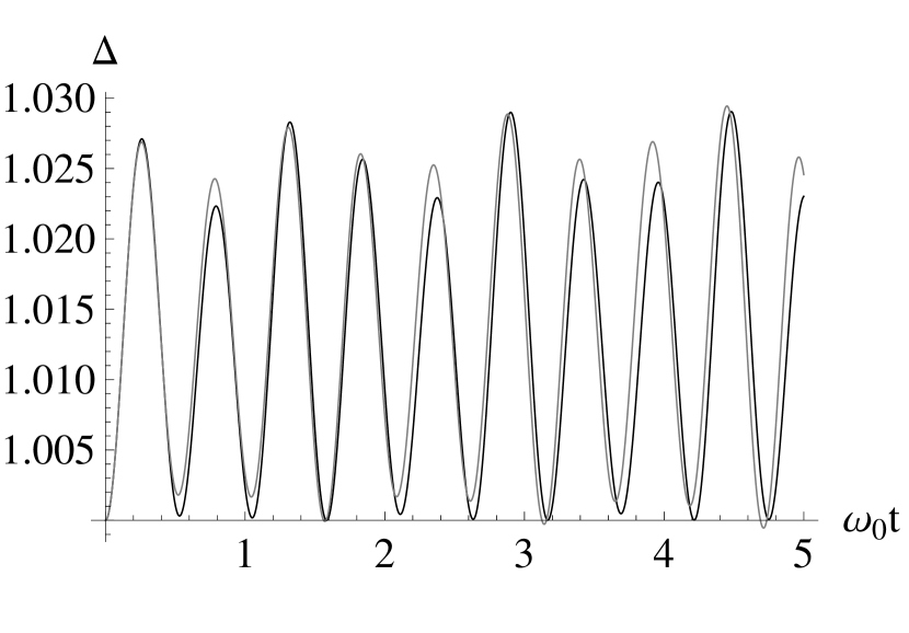
Figure 1: Phase space area as a function of time. Solid black: correlator approach to decoherence. Solid gray: master equation approach to decoherence. We use $\omega_{1}/\omega_{0}=2$, $\lambda/\omega_{0}^{2}=1/2$ and $\beta\omega_{0}=2000$.

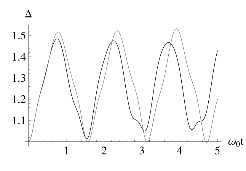
Figure 2: Phase space area as a function of time. Solid black: correlator approach to decoherence. Solid gray: master equation approach to decoherence. We use $\omega_{1}/\omega_{0}=2$, $\lambda/\omega_{0}^{2}=1/2$ and $\beta\omega_{0}=0.2$.

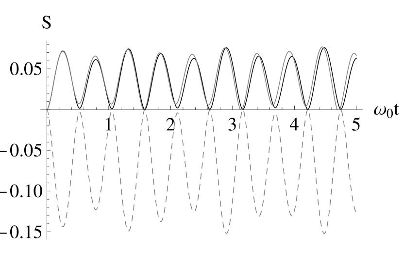
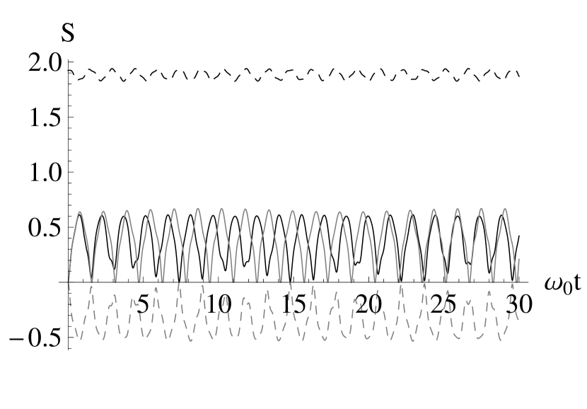
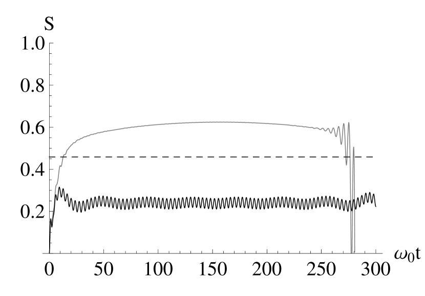
Figure 3: Entropy as a function of time. Solid black: correlator approach to decoherence, which follows from equation (18). Solid gray: master equation approach to decoherence. Dashed gray: correlation entropy, which follows from equation (19). We use $\omega_{1}/\omega_{0}=2$, $\lambda/\omega_{0}^{2}=1/2$ and $\beta\omega_{0}=2000$.

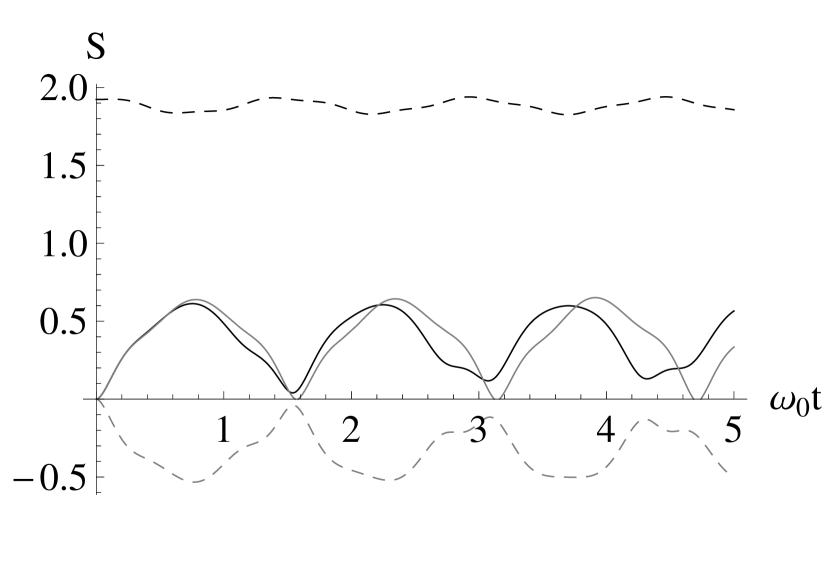
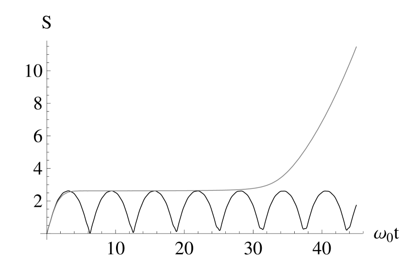
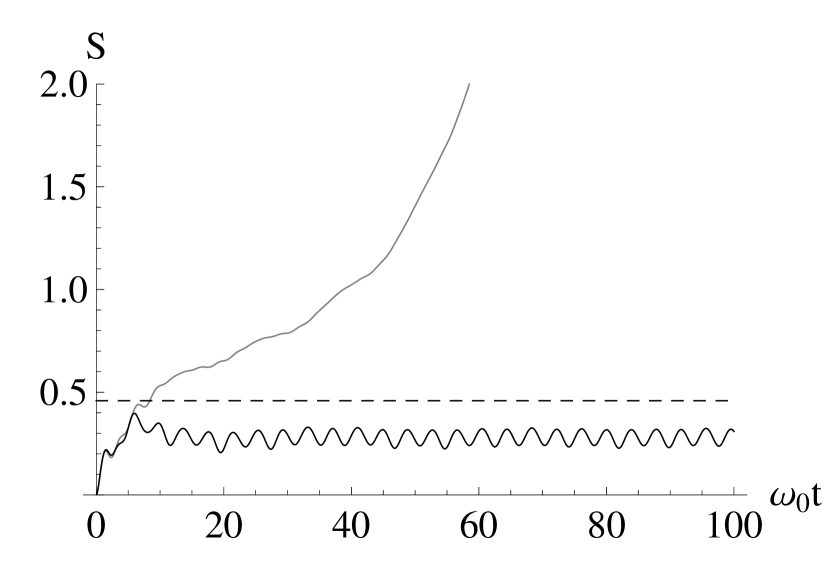
Figure 4: Entropy as a function of time. Solid black: correlator approach to decoherence. Solid gray: master equation approach to decoherence. Dashed black: entropy of the environment oscillator. Dashed gray: correlation entropy. We use $\omega_{1}/\omega_{0}=2$, $\lambda/\omega_{0}^{2}=1/2$ and $\beta\omega_{0}=0.2$.

Figure 5: Entropy as a function of time. Solid black: correlator approach to decoherence. Solid gray: master equation approach to decoherence. Dashed black: entropy of the environment oscillator. Dashed gray: correlation entropy. We use $\omega_{1}/\omega_{0}=2$, $\lambda/\omega_{0}^{2}=1/2$ and $\beta\omega_{0}=0.2$. The quasi periodic behaviour is due to Poincaré’s recurrence theorem.

Figure 6: Entropy as a function of time. Solid black: correlator approach to decoherence. Solid gray: master equation approach to decoherence. We use $\omega_{1}/\omega_{0}=201/200$, $\lambda/\omega_{0}^{2}=1/4$ and $\beta\omega_{0}=0.2$ such that we are in the resonant regime. The entropy as obtained from the master equation shows unphysical behaviour.

Let us begin by examining figures 6 and 6. In these figures we show the phase space area as a function of time for both the master equation approach to decoherence (gray) and our correlator approach to decoherence (black). In figure 6 the environment is, effectively, at $T=0$ as we use $\beta\omega_{0}=2000$. In figure 6 we use $\beta\omega_{0}=0.2$ such that the environmental oscillator is in “thermal equilibrium” at some finite temperature $k_{B}T=5\omega_{0}$. The difference between the two phase space areas is perturbatively small in both cases (the effective frequency that enters the master equation has been calculated by perturbative methods). In other words: both methods agree well. We can thus conclude that the entropy one obtains from the perturbative master equation in the Gaussian case in fact stems from neglecting the correlation entropy, just as in our correlator approach to decoherence.

As energy is conserved in our model, the Poincaré recurrence theorem applies. This theorem states that our system will after a sufficiently long time return to a state arbitrary close to its initial state. The Poincaré recurrence time is the amount of time this takes. In figure 6 we used almost commensurate eigenfrequencies. Consequently, the behaviour of the phase space area as a function of time is very regular. Introducing a non-zero temperature in figure 6 automatically makes the eigenfrequencies non-commensurate and thus induces a greater irregularity in the time evolution of the phase space area. In other words: the Poincaré recurrence time has increased.

Let us recall equation (17):

$$S_{\mathrm{vN}}=S_{\mathrm{total}}=S_{S}(t)+S_{E}(t)+S_{SE}(t)\,.$$

In figures 6, 6 and 6 we show the Gaussian von Neumann entropy for the system $S_{S}(t)$ (solid black) and for the environment $S_{E}(t)$ (dashed black), the Gaussian correlation entropy $S_{SE}(t)$ (dashed gray) and, finally, the entropy resulting from the master equation $S_{\mathrm{vN}}^{\mathrm{red}}(t)$ (solid gray). The solid black line in figure 6 is the entropy $S_{S}(t)$ one obtains from figure 6. Likewise, the solid black lines in figures 6 and 6 show the entropy $S_{S}(t)$ as a function of time one gets from figure 6. In figure 6 we show the behaviour up to very large times to nicely illustrate the quasi periodicity resulting from Poincaré’s recurrence theorem.

The dashed black lines in figures 6 and 6 show the environmental entropy $S_{E}(t)$. Just as $S_{S}(t)$, one can obtain $S_{E}(t)$ from the three non-trivial Gaussian correlators $\langle\hat{q}^{2}\rangle$, $\langle\hat{p}_{q}^{2}\rangle$ and $1/2\langle\{\hat{q},\hat{p}_{q}\}\rangle$ and by making use of equation (15). The environmental entropy in figure 6 is precisely equal to the system entropy $S_{S}(t)$ because both the system and the environment are at $T=0$. The dashed gray lines in figures 6, 6 and 6 show the Gaussian correlation entropy $S_{SE}(t)$ one obtains from equation (19). Finally, we can easily compare with the reduced von Neumann entropy one obtains from solving the master equation (in solid gray). Just as for the phase space area, the results differ only due to a small perturbative error in the master equation.

The oscillatory behaviour in the entropy can be interpreted in two ways:

• If one averages out the oscillations, the entropy of the system oscillator evolves from $S_{S}(0)=0$ to some small non-zero value $\overline{S}_{S}>0$, where $\overline{S}_{S}$ is the (classical) time average $\overline{S}_{S}=\langle S_{S}(t)\rangle$. This average non-zero value of the system entropy $\overline{S}_{S}$ exists by virtue of a negative correlation entropy. The amount of decoherence that the system has experienced thus equals $\overline{S}_{S}$;

• The Poincaré recurrence theorem enforces that the system returns arbitrarily close to its initial state after some finite Poincaré recurrence time. In quantum mechanics this recurrence time is rather small. This is not the case in field theoretical models as we discuss shortly.

So far, it is clear that the phase space area or the entropy in our correlator approach to decoherence and in the master equation approach to decoherence agree well up to perturbative corrections. Let us now examine the so-called resonant regime, where $\omega_{1}\simeq\omega_{0}$ in figure 6. Here, we set $\omega_{1}/\omega_{0}=201/200$. Our coupling is still small in this case so we are well in the perturbative regime where the master equation should yield sensible behaviour. Clearly, it does not as the entropy blows up. In the resonant regime the master equation suffers from secular growth which physically is not acceptable. Our approach indeed yields a perfectly finite evolution for the entropy.

Figure 7: Entropy as a function of time. Solid black: entropy of the system. Dashed black: entropy of the environment oscillator. We use $\omega_{1}/\omega_{0}=2$, $\lambda/\omega_{0}^{2}=1/4$ and $\beta$ is thus fixed via relation (43). The system entropy vanishes (pure state) and is time independent. The environmental entropy is a constant too. Despite that $\lambda\neq 0$, there are no oscillations in the expectation values as shown above.

In figure 7 we show the time evolution of the entropy for the time translation invariant initial conditions in equation (42) in our correlator approach to decoherence. Neither the entropy nor the phase space area change in time. We find this result rather interesting. Despite the fact that we are dealing with a non-zero coupling $\lambda\neq 0$, we can fine tune our initial conditions (42) such that there appears to be no influence of the coupling whatsoever when the entropy is measured. In other words, the expectation values in equation (42) are time independent and consequently fixed by their initial value despite of the coupling. This does not depend on how large the coupling $\lambda$ is.

V N Coupled Oscillators

We are really interested in the general case of $N$-oscillators. Let us consider the original Lagrangian in equation (4). We take $N=50$ throughout this section. In this section, we perform again two calculations:

• Decoherence in the conventional approach: we can numerically solve for the master equation in this case;

• Decoherence in our correlator approach: we can solve for the three non-trivial Gaussian system correlators by exact numerical methods from which we calculate the entropy.

Again does our simple action in equation (4) allow for a clean comparison of the two approaches to decoherence.

V.1 The Master Equation Approach to Decoherence

The form of the Paz-Zurek master equation itself remains unchanged of course and is given in equation (28) and (29). Compared to the previous section where we studied two oscillators only the precise form of the coefficients in equation (29) changes. Therefore, we exploit the same strategy as in the previous section and solve for the three non-trivial Gaussian correlators as in equation (39).

V.2 The Correlator Approach to Decoherence

The simplest way to study $N=50$ oscillators is not to diagonalise the resulting equation of motion (although this is of course possible in principle), but just study the unitary evolution of all Gaussian correlators in our system of interest by numerical methods. Let us recall the total Hamiltonian of our system of interest given in equation (23):

$$\hat{H}=\hat{H}_{S}+\hat{H}_{E}+\hat{H}_{\mathrm{Int}}=\frac{1}{2}\hat{p}_{x}^{2}+\frac{1}{2}\omega^{2}_{0}\hat{x}^{2}+\sum_{n=1}^{N}\left(\frac{1}{2}\hat{p}_{q_{n}}^{2}+\frac{1}{2}\omega_{n}^{2}\hat{q}_{n}^{2}+\lambda_{n}\hat{q}_{n}\hat{x}\right)\,.$$

Hamilton’s equations of motion thus yield:

$$\dot{\hat{x}} = \hat{p}_{x}$$ (44a)

$$\dot{\hat{p}}_{x} = -\omega_{0}^{2}\hat{x}-\sum_{n=1}^{N}\lambda_{n}\hat{q}_{n}$$ (44b)

$$\dot{\hat{q}}_{n} = \hat{p}_{q_{n}}$$ (44c)

$$\dot{\hat{p}}_{q_{n}} = -\omega_{n}^{2}\hat{q}_{n}-\lambda_{n}\hat{x}\,.$$ (44d)

We can thus straightforwardly derive the following set of coupled linear first order differential equations that govern the unitary time evolution of all Gaussian correlators:

$$\frac{\mathrm{d}\langle\hat{x}^{2}\rangle}{\mathrm{d}t} = 2\left\langle\frac{1}{2}\{\hat{x},\hat{p}_{x}\}\right\rangle$$ (45a)

$$\frac{\mathrm{d}\langle\hat{p}_{x}^{2}\rangle}{\mathrm{d}t} = -2\omega_{0}^{2}\left\langle\frac{1}{2}\{\hat{x},\hat{p}_{x}\}\right\rangle-2\sum_{n=1}^{N}\lambda_{n}\langle\hat{p}_{x}\hat{q}_{n}\rangle$$ (45b)

$$\frac{\mathrm{d}\left\langle\frac{1}{2}\{\hat{x},\hat{p}_{x}\}\right\rangle}{\mathrm{d}t} = -\omega_{0}^{2}\langle\hat{x}^{2}\rangle+\langle\hat{p}_{x}^{2}\rangle-\sum_{n=1}^{N}\lambda_{n}\langle\hat{x}\hat{q}_{n}\rangle$$ (45c)

$$\frac{\mathrm{d}\langle\hat{q}^{2}_{n}\rangle}{\mathrm{d}t} = 2\left\langle\frac{1}{2}\{\hat{q}_{n},\hat{p}_{q_{n}}\}\right\rangle$$ (45d)

$$\frac{\mathrm{d}\langle\hat{p}^{2}_{q_{n}}\rangle}{\mathrm{d}t} = -2\omega_{n}^{2}\left\langle\frac{1}{2}\{\hat{q}_{n},\hat{p}_{q_{n}}\}\right\rangle-2\lambda_{n}\langle\hat{p}_{q_{n}}\hat{x}\rangle$$ (45e)

$$\frac{\mathrm{d}\left\langle\frac{1}{2}\{\hat{q}_{n},\hat{p}_{q_{n}}\}\right\rangle}{\mathrm{d}t} = -\omega_{n}^{2}\langle\hat{q}^{2}_{n}\rangle+\langle\hat{p}^{2}_{q_{n}}\rangle-\lambda_{n}\langle\hat{x}\hat{q}_{n}\rangle$$ (45f)

$$\frac{\mathrm{d}\langle\hat{x}\hat{q}_{n}\rangle}{\mathrm{d}t} = \langle\hat{p}_{x}\hat{q}_{n}\rangle+\langle\hat{x}\hat{p}_{q_{n}}\rangle$$ (45g)

$$\frac{\mathrm{d}\langle\hat{p}_{x}\hat{q}_{n}\rangle}{\mathrm{d}t} = \langle\hat{p}_{x}\hat{p}_{q_{n}}\rangle-\omega_{0}^{2}\langle\hat{x}\hat{q}_{n}\rangle-\sum_{i=1}^{N}\lambda_{i}\langle\hat{q}_{i}\hat{q}_{n}\rangle$$ (45h)

$$\frac{\mathrm{d}\langle\hat{x}\hat{p}_{q_{n}}\rangle}{\mathrm{d}t} = \langle\hat{p}_{x}\hat{p}_{q_{n}}\rangle-\omega_{n}^{2}\langle\hat{x}\hat{q}_{n}\rangle-\lambda_{n}\langle\hat{x}^{2}\rangle$$ (45i)

$$\frac{\mathrm{d}\langle\hat{p}_{x}\hat{p}_{q_{n}}\rangle}{\mathrm{d}t} = -\omega_{0}^{2}\langle\hat{x}\hat{p}_{q_{n}}\rangle-\omega_{n}^{2}\langle\hat{p}_{x}\hat{q}_{n}\rangle-\lambda_{n}\left\langle\frac{1}{2}\{\hat{x},\hat{p}_{x}\}\right\rangle-\lambda_{n}\left\langle\frac{1}{2}\{\hat{q}_{n},\hat{p}_{q_{n}}\}\right\rangle-\sum_{\begin{subarray}{c}i=1\\ i\neq n\end{subarray}}^{N}\lambda_{i}\langle\hat{q}_{i}\hat{p}_{q_{n}}\rangle$$ (45j)

$$\frac{\mathrm{d}\langle\hat{q}_{n}\hat{q}_{m}\rangle}{\mathrm{d}t} = \langle\hat{q}_{n}\hat{p}_{q_{m}}\rangle+\langle\hat{q}_{m}\hat{p}_{q_{n}}\rangle$$ (45k)

$$\frac{\mathrm{d}\langle\hat{q}_{n}\hat{p}_{q_{m}}\rangle}{\mathrm{d}t} = \langle\hat{p}_{q_{n}}\hat{p}_{q_{m}}\rangle-\omega_{m}^{2}\langle\hat{q}_{n}\hat{q}_{m}\rangle-\lambda_{m}\langle\hat{x}\hat{q}_{n}\rangle$$ (45l)

$$\frac{\mathrm{d}\langle\hat{p}_{q_{n}}\hat{p}_{q_{m}}\rangle}{\mathrm{d}t} = -\omega_{n}^{2}\langle\hat{q}_{n}\hat{p}_{q_{m}}\rangle-\omega_{m}^{2}\langle\hat{q}_{m}\hat{p}_{q_{n}}\rangle-\lambda_{n}\langle\hat{x}\hat{p}_{q_{m}}\rangle-\lambda_{m}\langle\hat{x}\hat{p}_{q_{n}}\rangle\,.$$ (45m)

In the last three equations $m\neq n$ is implied. In other words, for $m=n$, we would find equations (45d), (45e) and (45f) again. As in the previous section, we require “pure-thermal” initial conditions. They generalise to:

$$\begin{array}[]{lllllll}\langle\hat{x}^{2}(t_{0})\rangle=\frac{1}{2\omega_{0}}&\phantom{1}&\langle\hat{p}_{x}^{2}(t_{0})\rangle=\frac{\omega_{0}}{2}&\phantom{1}&\langle\{\hat{x}(t_{0}),\hat{p}_{x}(t_{0})\}\rangle=0&\phantom{1}&\phantom{1}\\ \langle\hat{q}^{2}_{n}(t_{0})\rangle=\frac{1}{2\omega_{n}}\coth\left(\frac{\beta\omega_{n}}{2}\right)&\phantom{1}&\langle\hat{p}_{q_{n}}^{2}(t_{0})\rangle=\frac{\omega_{n}}{2}\coth\left(\frac{\beta\omega_{n}}{2}\right)&\phantom{1}&\langle\{\hat{q}_{n}(t_{0}),\hat{p}_{q_{n}}(t_{0})\}\rangle=0&\phantom{1}&\phantom{1}\\ \langle\hat{x}(t_{0})\hat{q}_{n}(t_{0})\rangle=0&\phantom{1}&\langle\hat{p}_{x}(t_{0})\hat{p}_{q_{n}}(t_{0})\rangle=0&\phantom{1}&\langle\hat{x}(t_{0})\hat{p}_{q_{n}}(t_{0})\rangle=0&\phantom{1}&\langle\hat{q}_{n}(t_{0})\hat{p}_{x}(t_{0})\rangle=0\\ \langle\hat{q}_{n}(t_{0})\hat{q}_{m}(t_{0})\rangle=0&\phantom{1}&\langle\hat{p}_{q_{n}}(t_{0})\hat{p}_{q_{m}}(t_{0})\rangle=0&\phantom{1}&\langle\hat{q}_{n}(t_{0})\hat{p}_{q_{m}}(t_{0})\rangle=0\,,&\phantom{1}&\phantom{1}\end{array}$$ (46)

where of course $1\leq\{n,m\}\leq N$, $m\neq n$. For simplicity we will restrict ourselves to the case where $\lambda=\lambda_{n}$, $1\leq n\leq N$, throughout the paper.

V.3 Results

Figure 8: Entropy as a function of time. Solid black: correlator approach to decoherence. Solid gray: master equation approach to decoherence. We use $\omega_{n}/\omega_{0}\in[2,3]$, $\lambda/\omega_{0}^{2}=1/8$ and $\beta\omega_{0}=2$.

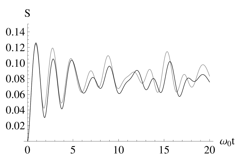
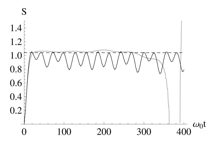
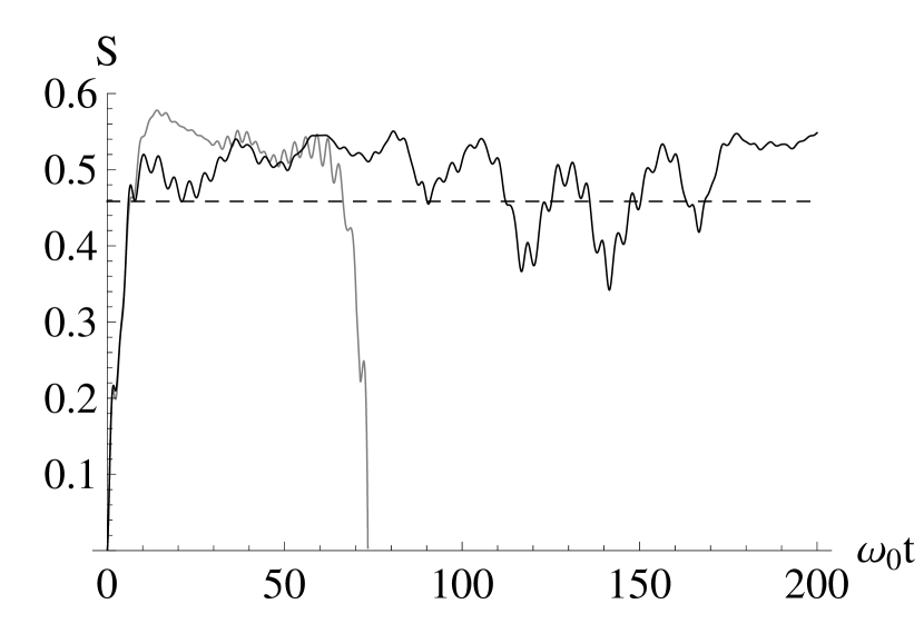
Figure 9: Entropy as a function of time. Solid black: correlator approach to decoherence. Solid gray: master equation approach to decoherence. We use $\omega_{n}/\omega_{0}\in[9/10,11/10]$, $\lambda/\omega_{0}^{2}=1/40$ and $\beta\omega_{0}=1$. The dashed black line indicates complete thermalisation (perfect decoherence).

Figure 10: Entropy as a function of time. Solid black: correlator approach to decoherence. Solid gray: master equation approach to decoherence. We use $\omega_{n}/\omega_{0}=1+n/50$, $\lambda/\omega_{0}^{2}=3/40$ and $\beta\omega_{0}=2$.

Figure 11: Entropy as a function of time. Solid black: correlator approach to decoherence. Solid gray: master equation approach to decoherence. We use $\omega_{n}/\omega_{0}=1+n/100$, $\lambda/\omega_{0}^{2}=3/40$ and $\beta\omega_{0}=2$.

Figure 12: Entropy as a function of time. Solid black: correlator approach to decoherence. Solid gray: master equation approach to decoherence. We use $\omega_{n}/\omega_{0}\in[3/4,3/2]$, $\lambda/\omega_{0}^{2}=1/16$ and $\beta\omega_{0}=2$.

Figure 13: Entropy as a function of time. Solid black: correlator approach to decoherence. Solid gray: master equation approach to decoherence. We use $\omega_{n}/\omega_{0}\in[19/20,21/20]$, $\lambda/\omega_{0}^{2}=1/10$ and $\beta\omega_{0}=1/10$. At such a high environmental temperature we generate a significant amount of entropy.

We consider $N=50$ environmental oscillators. Let us firstly present a case where the master equation produces accurate results. In figure 13 we show the evolution of the entropy obtained from the master equation (solid gray) and in our correlator approach to decoherence (solid black). We randomly generate the environmental frequencies $\omega_{n}/\omega_{0}$, with $1\leq n\leq N$, in the interval between 2 and 3. Henceforth, we denote this by $\omega_{n}/\omega_{0}\in[2,3]$. With $\lambda/\omega_{0}^{2}=1/8$ this case is clearly deep in the perturbative regime away from resonance frequencies as all environmental frequencies are larger than the system frequency. Only a little entropy is generated so virtually no decoherence has taken place compared to the thermal value the entropy can reach in principle if decoherence is effective. Indeed, given some temperature of the environment, the thermal value of the entropy provides us with a reasonable estimate for the upper limit the entropy can reach. For the parameters under consideration, we have a thermal entropy $S_{\mathrm{th}}\simeq 0.458$ as $\beta\omega_{0}=2$, whereas the average generated entropy is only of the order of $\overline{S}_{S}\simeq 0.08$. This case is thus not very different from a $T=0$ evolution. Our system has not decohered as the environmental frequencies are all larger than the system frequency, the coupling is weak and the temperature of the environment is low. In other words, the system and environmental oscillators are virtually decoupled from each other.

Let us now consider figure 13. Here, we used $\omega_{n}/\omega_{0}\in[9/10,11/10]$ with $1\leq n\leq N$. These frequencies are thus randomly spaced around $\omega_{0}$ in a small interval. As all frequencies are close to each other, we expect that thermalisation and decoherence occur swiftly and effectively, unlike in the previous case we considered. At early times $0\leq\omega_{0}t\lesssim 15$, we see that the entropy calculated from the master equation and our correlator approach to decoherence coincide nicely. This is to be expected as the perturbative master equation should yield the correct early time evolution. In other words: it is possible to extract the relevant decoherence time scale correctly from both the master equation and from our correlator approach to decoherence.

As entropy or the phase space area quantifies the amount of decoherence, the rate of change of the phase space area quantifies the decoherence rate $\Gamma$. We can determine $\Gamma$ at each moment in time formally by solving:

$$\dot{\Delta}(t)+\Gamma(t)\Delta(t)=0\,.$$ (47)

Due to the oscillatory nature of the phase space area as a function of time, one should average over a conveniently chosen time interval to sensibly determine for example the decoherence rate at early times. In this quantum mechanical example it is not possible to find a simple (time independent) analytic expression for $\Gamma$, whereas in the field theoretical model we investigated $\Gamma$ is very well approximated by the tree level decay rate Koksma:2009wa . In Zurek:2003zz one can find a decoherence time for this model that depends on the spatial coordinates of the density matrix. We do not find an invariant measure of the decoherence rate of that type.

Now, let us turn our attention to the late time behaviour in figure 13. Around $\omega_{0}t\simeq 280$ the master equation suddenly destabilises and the entropy becomes ill defined in the sense that the effective phase space area of the state becomes negative. One can easily check that the 51 eigenfrequencies one obtains by rotating to the diagonal frame, analogous to equation (53) for $N=1$, are all positive so the resulting evolution should be stable. Clearly, this signals a breakdown of the perturbative master equation.

The latter seems to be a generic feature of the perturbative master equation in the resonant regime. Let us consider the figures 13, 13, 13 and 13. In figure 13 we use $\omega_{n}/\omega_{0}=1+n/50$, in figure 13 we use $\omega_{n}/\omega_{0}=1+n/100$, in figure 13: $\omega_{n}/\omega_{0}\in[3/4,3/2]$ and in figure 13: $\omega_{n}/\omega_{0}\in[19/20,21/20]$. Independently on how precisely one chooses the distribution of environmental frequencies, the perturbative master equation breaks down. In all these cases are the eigenfrequencies positive, and we are in all cases in the perturbative regime, so the evolution of the entropy should be regular at all times.

The system’s entropy should asymptote to the thermal entropy if thermalisation is complete which we indicate by the dashed black line in all the figures in this section. A perfectly thermalised state corresponds to a maximally decohered state and consequently an imperfectly thermalised state corresponds to a partially decohered state. Averaging out the oscillations of our unitary evolution in e.g. figure 13 yields an average value of the entropy that is below this thermal value. This can be expected given the fact that our coupling is very small $\lambda/\omega_{0}^{2}=3/40$. Also, one can verify that the energy is conserved by the evolution as it should.

However, the master equation in figure 13 yields a stationary entropy that is larger than the thermal value, indicating that the temperature of the system would be higher than the environmental temperature. Clearly, this does not make sense. The two most important quantitative measures of decoherence one hopes to extract out of an experiment or a calculation are the decoherence rate and the total generated entropy as the latter tells us how much decoherence has taken place and how classical the state has become, and the former how fast this state is reached. We conclude that for this choice of parameters the total generated entropy at late times does not follow correctly from the master equation. We checked that this failure of the master equation is generic. Even in the case of figure 13, we see that although the asymptote is roughly equal to the thermal value in the range $25\lesssim\omega_{0}t\lesssim 280$, it is too high based on our exact numerical analysis ($\overline{S}_{S}<S_{\mathrm{th}}$).

The oscillations in the entropy as a function of time that are present in our exact evolution are not present in the evolution of the entropy that follows from the master equation. The master equation thus tends to overdamp oscillations in expectation values.

Finally, compared to the $N=1$ case we previously considered, we observe that Poincaré’s recurrence time has dramatically increased. For example in figure 13 one has to wait for a very long time before a random fluctuation decreases the entropy significantly again to values close to its initial value. Thus, by including more oscillators decoherence becomes rapidly more irreversible, as one would expect.

VI Conclusion

Decoherence is often studied by considering a perturbative master equation. This approach suffers from both theoretical and practical shortcomings. It is unsatisfactory that $\rho_{\mathrm{red}}$ evolves non-unitarily while the underlying theory (quantum mechanics or quantum field theory) is unitary. We are not against non-unitary equations or approximations in principle, however, one should make sure that the essential physical features of the system one is describing are kept. The master equations does not break unitarity correctly, as we have shown in this paper. On the practical side, the master equation is so complex that field theoretical questions have barely been addressed: there does not exist a treatment to take perturbative interactions properly into account, nor has any reduced density matrix ever been renormalised. Moreover, as we show in this paper, the perturbative master equations leads even in simple situations in quantum mechanics to physically unacceptable behaviour. Although for early times the entropy increases, for late times the approach fails and suffers from secular growth as the entropy continues to grow without bound. This behaviour is generic when at least some of the environmental oscillators are in the resonant regime. Of course one could argue that we should have solved the non-perturbative master equation in the resonant regime. Although true in principle, the point of this paper is that it is much more convenient on theoretical and practical grounds to solve for correlators than for density matrices.

We advocate a novel approach to decoherence based on neglecting information in observationally unaccessible correlators. If proper interactions (non-Gaussianities) are taken into account, neglecting the information stored in higher order non-Gaussian correlators gives rise to an increase in the Gaussian von Neumann entropy. In this paper we consider a quadratic model of $N$ coupled simple harmonic oscillators where no non-Gaussianities are generated. Due to the non-zero coupling however, an increase in the Gaussian von Neumann entropy can be observed at the expense of a negative correlation entropy as the total von Neumann entropy is constant in unitary theories.

In this paper we study a quadratic model where the trace can be performed, where the perturbative master equation can be solved and where there is no need to renormalise as we study decoherence in a quantum mechanical setting. We can thus circumvent the practical drawbacks that usually prevent us from solving the perturbative master equation in a renormalised interacting quantum field theoretical model. In this simple quadratic quantum mechanical model, we can thus actually compare the master equation approach to decoherence and our correlator approach to decoherence. From the numerical analysis we conclude:

• Away from the resonant regime, where all $\omega_{n}$ significantly differ from $\omega_{0}$, the evolution of the entropy in the master equation approach and in our correlator approach to decoherence agree nicely (up to the expected perturbative corrections). The system decoheres only weakly in this regime however. The two approaches also agree nicely at very early times such that both approaches can be used to accurately calculate decoherence rates;

• In the resonant regime, where a certain number of $\omega_{n}\simeq\omega_{0}$, the perturbative master equation breaks down despite of the fact that we are still in the perturbative regime and despite of the fact that all eigenfrequencies are positive. The value to which the entropy asymptotes in the master equation approach before the breakdown is reached is generically too high. This leads to an inaccurate prediction of the amount of decoherence that has taken place. In some cases, the breakdown occurs already before this asymptotic state has been reached;

• The evolution of the entropy in both the resonant and in the non-resonant regime in our correlator approach to decoherence behaves perfectly finite. The late time asymptote that is eventually reached either indicates perfect thermalisation (maximal decoherence) or, for smaller values of the coupling and a finite number of environmental oscillators, imperfect thermalisation (imperfect decoherence).

Our correlator approach to decoherence thus provides us with a new insight in the conventional approach to decoherence. If the entropy from the master equation agrees with our exact Gaussian von Neumann entropy up to perturbative corrections, then one neglects the information stored in the system-environment correlators in the conventional approach to decoherence too.

There are generally speaking two quantitative results that can be obtained after performing an experiment or a calculation concerning decoherence:

• Decoherence rate;

• Total amount of decoherence.

We argue that one should use the entropy (or, equivalently, the phase space area) to quantify these two aspects of decoherence. The decoherence rate $\Gamma$ is the rate at which the phase space area changes and can formally be obtained from solving equation (47). The total amount of entropy generated measures the total amount of decoherence that has occurred. At late times we have seen that, upon averaging out the oscillations, a thermal state is maximally decohered. This agrees perfectly with the point of view where a reduced density matrix whose off diagonal elements (in the observer’s basis) have disappeared corresponds to a classical state. A (free) thermal density matrix follows from equations (10b) and (13) as:

$$\rho_{\mathrm{th}}(x,y;t)={\cal N}_{\mathrm{th}}(t)\exp\left[-\frac{\Delta_{\mathrm{th}}^{2}}{8\langle\hat{x}^{2}\rangle_{\mathrm{th}}}\left(x-y\right)^{2}-\frac{1}{8\langle\hat{x}^{2}\rangle_{\mathrm{th}}}\left(x+y\right)^{2}\right]\,.$$ (48)

The thermal correlators can be read off for example from equation (41). Clearly, at high temperatures we have that $\Delta_{\mathrm{th}}\gg 1$ such that the off diagonal terms in the density matrix have almost disappeared. The classical limit of quantum mechanics in not classical mechanics but rather classical stochastic mechanics. Likewise the classical limit of quantum field theory (in a thermal environment) is not classical field theory but classical stochastic field theory. This implies that a particular measurement does not yield a certain predetermined outcome but rather a certain outcome that is randomly drawn from a probability distribution function of uncorrelated or not entangled possibilities.

We can learn several things about decoherence in field theories from our quantum mechanical analysis. Firstly, the reason why the perturbative master equation fails in the resonant regime is that the quadratic coupling between system and environment is treated on equal footing as a proper non-Gaussian interaction. In the perturbative master equation, one attempts to solve the following “interaction” in the “Kadanoff-Baym” equations:

$$\includegraphics[width=85.35826pt]{Feynmandiagram.eps}\quad+\quad\includegraphics[width=85.35826pt]{Feynmandiagram2.eps}\quad+\ldots\,.$$ (49)

Of course, this is not a proper interaction and the 1 particle irreducible (1PI) self-mass that enters the Kadanoff-Baym equations due to such a quadratic coupling vanishes. In this simple quantum mechanical example, one should therefore just solve for the correlators following from the von Neumann equation exactly as we showed in this paper. We thus also accounted for the backreaction from the system on the environment. The set of Kadanoff-Baym equations is the sophisticated machinery to properly solve for the propagators in an interacting quantum field theory. Only the diagrams that follow from a 2PI effective action contribute. As is well known, the Kadanoff-Baym equations resum Feynman diagrams and prevent secular terms from developing. This leads to a stable, thermalised late time behaviour (see Berges:2000ur ; Berges:2004yj ; Calzetta:book ). Secondly, for $N=1$ and for almost commensurate eigenfrequencies, we have seen that Poincaré’s recurrence time is rather small: the system returns rather quickly to its initial state. For non-commensurate eigenfrequencies Poincaré’s recurrence time increases. For $N=50$ we have seen that Poincaré’s recurrence time dramatically increases such that we have to wait for a much longer time before the system returns to a state arbitrarily close to its initial state. There are two complementary ways to interpret this observation. One could take the point of view that our system has experienced an average entropy increase, e.g. $0<\overline{S}_{S}\lesssim S_{\mathrm{th}}$, where $\overline{S}_{S}$ is the classical time average of $S_{S}(t)$. In other words, the system has experienced a total amount of decoherence equal to $\overline{S}_{S}$. Alternatively, one can say that since the Poincaré recurrence time is still finite, although large, no irreversible process of decoherence has taken place as the system returns arbitrarily close to its initial state again. In an interacting field theory several modes couple due to the loop integrals (hence $N\rightarrow\infty$) and clearly our Poincaré recurrence time becomes infinite. Hence, the entropy increase has become irreversible (for all practical purposes) and our system has decohered.

We hope to generalise the analysis presented here to a quantum mechanical interaction that comes closer to field theory but is still free from divergences. In particular, we will consider entropy generation in a quantum mechanical $\lambda xq^{2}$ model, which, when analysed by making use of the master equation, is very similar to the present $\lambda xq$ model after $q$ has been integrated out Hu:1993vs . The purpose of introducing our novel approach to decoherence is not to study quadratic quantum mechanical models, but proper interacting field theories, like in Koksma:2009wa .

Appendix A The Statistical Propagator for $N=1$

Let us now return to the lagrangian (36) from which it follows that the equation of motion for the two oscillators can be written in matrix form as:

$$\frac{\mathrm{d}^{2}}{\mathrm{d}t^{2}}\vec{q}+\Omega\vec{q}=0\,,$$ (50)

where:

$$\Omega=\left(\begin{array}[]{cc}\omega_{0}^{2}&\lambda_{1}\\ \lambda_{1}&\omega_{1}^{2}\end{array}\right)$$ (51)

and where we employed the notation $\vec{q}^{\,\,\mathrm{T}}=(x,q)$. We can now easily diagonalise the equation of motion:

$$\frac{\mathrm{d}^{2}}{\mathrm{d}t^{2}}\vec{q}_{\mathrm{d}}+\Omega_{\mathrm{d}}\vec{q}_{\mathrm{d}}=0\,,$$ (52)

where we diagonalised the system by making use of the rotation matrix $R$:

$$\Omega_{\mathrm{d}}=R\Omega R^{T}=\left(\begin{array}[]{cc}\bar{\omega}_{0}^{2}&0\cr 0&\bar{\omega}_{1}^{2}\cr\end{array}\right)=\left(\begin{array}[]{cc}\frac{1}{2}(\omega_{0}^{2}+\omega_{1}^{2})-\frac{1}{2}\sqrt{(\omega_{1}^{2}-\omega_{0}^{2})^{2}+4\lambda_{1}^{2}}&0\cr 0&\frac{1}{2}(\omega_{0}^{2}+\omega_{1}^{2})+\frac{1}{2}\sqrt{(\omega_{1}^{2}-\omega_{0}^{2})^{2}+4\lambda_{1}^{2}}\cr\end{array}\right)\,,$$ (53)

with:

$$R=\left(\begin{array}[]{cc}\cos(\theta)&-\sin(\theta)\cr\sin(\theta)&\cos(\theta)\cr\end{array}\right)\,.$$ (54)

Moreover, we defined:

$$\vec{q}_{\mathrm{d}}(t)=\left(\begin{array}[]{c}\bar{x}(t)\cr\bar{q}(t)\cr\end{array}\right)=\left(\begin{array}[]{c}\cos(\theta)x(t)-\sin(\theta)q(t)\cr\sin(\theta)x(t)+\cos(\theta)q(t)\cr\end{array}\right)\,.$$ (55)

Finally, one can derive that:

$$\cos(2\theta) = \frac{\omega_{1}^{2}-\omega_{0}^{2}}{\sqrt{(\omega_{1}^{2}-\omega_{0}^{2})^{2}+4\lambda_{1}^{2}}}$$ (56a)

$$\sin(2\theta) = \frac{2\lambda_{1}}{\sqrt{(\omega_{1}^{2}-\omega_{0}^{2})^{2}+4\lambda_{1}^{2}}}\,.$$ (56b)

In order for the system to be stable we should have $\bar{\omega}_{0}^{2}\geq 0$, which implies $\lambda_{1}\leq\omega_{0}\omega_{1}$. When $\lambda_{1}>\omega_{0}\omega_{1}$ the upper eigenmode corresponds to an inverted harmonic oscillator, $\bar{\omega}_{0}^{2}<0$, and we shall not consider this case here. We can immediately solve the equation of motion in the diagonal frame:

$$\vec{q}_{\mathrm{d}}(t)=\left(\begin{array}[]{c}\bar{x}(t)\cr\bar{q}(t)\cr\end{array}\right)=\left(\begin{array}[]{c}A_{0}\cos(\bar{\omega}_{0}t)+B_{0}\sin(\bar{\omega}_{0}t)\cr A_{1}\cos(\bar{\omega}_{1}t)+B_{1}\sin(\bar{\omega}_{1}t)\cr\end{array}\right)\,,$$ (57)

We do not yet impose initial conditions for the coefficients in this solution, but rather first solve for the statistical propagator for the system:

$$F_{x}(t;t^{\prime}) = \frac{1}{2}\mathrm{Tr}\left[\hat{\rho}(t_{0})\{\hat{x}(t^{\prime}),\hat{x}(t)\}\right]=\frac{1}{2}\langle\{\hat{x}(t^{\prime}),\hat{x}(t)\}\rangle$$

$$= \frac{1}{2}\Big{[}\cos^{2}(\theta)\langle\{\hat{\bar{x}}(t^{\prime}),\hat{\bar{x}}(t)\}\rangle+\sin^{2}(\theta)\langle\{\hat{\bar{q}}(t^{\prime}),\hat{\bar{q}}(t)\}\rangle+\cos(\theta)\sin(\theta)\langle\{\hat{\bar{x}}(t^{\prime}),\hat{\bar{q}}(t)\}+\{\hat{\bar{q}}(t^{\prime}),\hat{\bar{x}}(t)\}\rangle\Big{]}\,.$$

Inserting the solution (57) yields the general form for the statistical propagator:

$$F_{x}(t;t^{\prime})=$$ (59)

$$\cos^{2}(\theta)\Big{\{}\langle\hat{A}_{0}^{2}\rangle\cos(\bar{\omega}_{0}t)\cos(\bar{\omega}_{0}t^{\prime})+\langle\hat{B}_{0}^{2}\rangle\sin(\bar{\omega}_{0}t)\sin(\bar{\omega}_{0}t^{\prime})+\frac{\langle\{\hat{A}_{0},\hat{B}_{0}\}\rangle}{2}\left(\cos(\bar{\omega}_{0}t)\sin(\bar{\omega}_{0}t^{\prime})+\sin(\bar{\omega}_{0}t)\cos(\bar{\omega}_{0}t^{\prime})\right)\Big{\}}$$

$$+\sin^{2}(\theta)\Big{\{}\langle\hat{A}_{1}^{2}\rangle\cos(\bar{\omega}_{1}t)\cos(\bar{\omega}_{1}t^{\prime})+\langle\hat{B}_{1}^{2}\rangle\sin(\bar{\omega}_{1}t)\sin(\bar{\omega}_{1}t^{\prime})+\frac{\langle\{\hat{A}_{1},\hat{B}_{1}\}\rangle}{2}\left(\cos(\bar{\omega}_{1}t)\sin(\bar{\omega}_{1}t^{\prime})+\sin(\bar{\omega}_{1}t)\cos(\bar{\omega}_{1}t^{\prime})\right)\!\Big{\}}$$

$$+\frac{\sin(2\theta)}{4}\Big{\{}\langle\{\hat{A}_{0},\hat{A}_{1}\}\rangle\left(\cos(\bar{\omega}_{0}t)\cos(\bar{\omega}_{1}t^{\prime})+\cos(\bar{\omega}_{1}t)\cos(\bar{\omega}_{0}t^{\prime})\right)+\langle\{\hat{B}_{0},\hat{B}_{1}\}\rangle\left(\sin(\bar{\omega}_{0}t)\sin(\bar{\omega}_{1}t^{\prime})+\sin(\bar{\omega}_{1}t)\sin(\bar{\omega}_{0}t^{\prime})\right)$$

$$\qquad\quad+\langle\{\hat{A}_{0},\hat{B}_{1}\}\rangle\left(\cos(\bar{\omega}_{0}t)\sin(\bar{\omega}_{1}t^{\prime})+\sin(\bar{\omega}_{1}t)\cos(\bar{\omega}_{0}t^{\prime})\right)+\langle\{\hat{B}_{0},\hat{A}_{1}\}\rangle\left(\sin(\bar{\omega}_{0}t)\cos(\bar{\omega}_{1}t^{\prime})+\cos(\bar{\omega}_{1}t)\sin(\bar{\omega}_{0}t^{\prime})\right)\Big{\}}.$$

Similarly, we can derive the statistical propagator for the environment:

$$F_{q}(t;t^{\prime}) = \frac{1}{2}\mathrm{Tr}\left[\hat{\rho}(t_{0})\{\hat{q}(t^{\prime}),\hat{q}(t)\}\right]=\frac{1}{2}\langle\{\hat{q}(t^{\prime}),\hat{q}(t)\}\rangle$$

$$= \frac{1}{2}\Big{[}\sin^{2}(\theta)\langle\{\hat{\bar{x}}(t^{\prime}),\hat{\bar{x}}(t)\}\rangle+\cos^{2}(\theta)\langle\{\hat{\bar{q}}(t^{\prime}),\hat{\bar{q}}(t)\}\rangle-\cos(\theta)\sin(\theta)\langle\{\hat{\bar{x}}(t^{\prime}),\hat{\bar{q}}(t)\}+\{\hat{\bar{q}}(t^{\prime}),\hat{\bar{x}}(t)\}\rangle\Big{]}\,,$$

such that we find:

$$F_{q}(t;t^{\prime})=$$ (61)

$$\sin^{2}(\theta)\Big{\{}\langle\hat{A}_{0}^{2}\rangle\cos(\bar{\omega}_{0}t)\cos(\bar{\omega}_{0}t^{\prime})+\langle\hat{B}_{0}^{2}\rangle\sin(\bar{\omega}_{0}t)\sin(\bar{\omega}_{0}t^{\prime})+\frac{\langle\{\hat{A}_{0},\hat{B}_{0}\}\rangle}{2}\left(\cos(\bar{\omega}_{0}t)\sin(\bar{\omega}_{0}t^{\prime})+\sin(\bar{\omega}_{0}t)\cos(\bar{\omega}_{0}t^{\prime})\right)\Big{\}}$$

$$+\cos^{2}(\theta)\Big{\{}\langle\hat{A}_{1}^{2}\rangle\cos(\bar{\omega}_{1}t)\cos(\bar{\omega}_{1}t^{\prime})+\langle\hat{B}_{1}^{2}\rangle\sin(\bar{\omega}_{1}t)\sin(\bar{\omega}_{1}t^{\prime})+\frac{\langle\{\hat{A}_{1},\hat{B}_{1}\}\rangle}{2}\left(\cos(\bar{\omega}_{1}t)\sin(\bar{\omega}_{1}t^{\prime})+\sin(\bar{\omega}_{1}t)\cos(\bar{\omega}_{1}t^{\prime})\right)\!\Big{\}}$$

$$-\frac{\sin(2\theta)}{4}\Big{\{}\langle\{\hat{A}_{0},\hat{A}_{1}\}\rangle\left(\cos(\bar{\omega}_{0}t)\cos(\bar{\omega}_{1}t^{\prime})+\cos(\bar{\omega}_{1}t)\cos(\bar{\omega}_{0}t^{\prime})\right)+\langle\{\hat{B}_{0},\hat{B}_{1}\}\rangle\left(\sin(\bar{\omega}_{0}t)\sin(\bar{\omega}_{1}t^{\prime})+\sin(\bar{\omega}_{1}t)\sin(\bar{\omega}_{0}t^{\prime})\right)$$

$$\qquad\quad+\langle\{\hat{A}_{0},\hat{B}_{1}\}\rangle\left(\cos(\bar{\omega}_{0}t)\sin(\bar{\omega}_{1}t^{\prime})+\sin(\bar{\omega}_{1}t)\cos(\bar{\omega}_{0}t^{\prime})\right)+\langle\{\hat{B}_{0},\hat{A}_{1}\}\rangle\left(\sin(\bar{\omega}_{0}t)\cos(\bar{\omega}_{1}t^{\prime})+\cos(\bar{\omega}_{1}t)\sin(\bar{\omega}_{0}t^{\prime})\right)\Big{\}}.$$

Finally, we need the statistical propagator for the system-environment correlations:

$$F_{xq}(t;t^{\prime}) = \frac{1}{2}\mathrm{Tr}\left[\hat{\rho}(t_{0})\{\hat{x}(t^{\prime}),\hat{q}(t)\}\right]=\frac{1}{2}\langle\{\hat{x}(t^{\prime}),\hat{q}(t)\}\rangle$$

$$= \frac{1}{2}\Big{[}\frac{\sin(2\theta)}{2}\left(\langle\{\hat{\bar{q}}(t^{\prime}),\hat{\bar{q}}(t)\}\rangle-\langle\{\hat{\bar{x}}(t^{\prime}),\hat{\bar{x}}(t)\}\rangle\right)+\cos^{2}(\theta)\langle\{\hat{\bar{x}}(t^{\prime}),\hat{\bar{q}}(t)\}\rangle-\sin^{2}(\theta)\langle\{\hat{\bar{q}}(t^{\prime}),\hat{\bar{x}}(t)\}\rangle\Big{]}\,,$$

which in turn yields:

$$F_{xq}(t;t^{\prime})=$$ (63)

$$\frac{\sin(2\theta)}{2}\Big{\{}\langle\hat{A}_{1}^{2}\rangle\cos(\bar{\omega}_{1}t)\cos(\bar{\omega}_{1}t^{\prime})+\langle\hat{B}_{1}^{2}\rangle\sin(\bar{\omega}_{1}t)\sin(\bar{\omega}_{1}t^{\prime})+\frac{\langle\{\hat{A}_{1},\hat{B}_{1}\}\rangle}{2}\left(\cos(\bar{\omega}_{1}t)\sin(\bar{\omega}_{1}t^{\prime})+\sin(\bar{\omega}_{1}t)\cos(\bar{\omega}_{1}t^{\prime})\right)$$

$$\qquad\qquad-\langle\hat{A}_{0}^{2}\rangle\cos(\bar{\omega}_{0}t)\cos(\bar{\omega}_{0}t^{\prime})-\langle\hat{B}_{0}^{2}\rangle\sin(\bar{\omega}_{0}t)\sin(\bar{\omega}_{0}t^{\prime})-\frac{\langle\{\hat{A}_{0},\hat{B}_{0}\}\rangle}{2}\left(\cos(\bar{\omega}_{0}t)\sin(\bar{\omega}_{0}t^{\prime})+\sin(\bar{\omega}_{0}t)\cos(\bar{\omega}_{0}t^{\prime})\right)\!\Big{\}}$$

$$+\frac{\cos^{2}(\theta)}{2}\Big{\{}\langle\{\hat{A}_{0},\hat{A}_{1}\}\rangle\cos(\bar{\omega}_{1}t)\cos(\bar{\omega}_{0}t^{\prime})+\langle\{\hat{B}_{0},\hat{B}_{1}\}\rangle\sin(\bar{\omega}_{1}t)\sin(\bar{\omega}_{0}t^{\prime})$$

$$\qquad\qquad\qquad\qquad+\langle\{\hat{A}_{0},\hat{B}_{1}\}\rangle\sin(\bar{\omega}_{1}t)\cos(\bar{\omega}_{0}t^{\prime})+\langle\{\hat{B}_{0},\hat{A}_{1}\}\rangle\cos(\bar{\omega}_{1}t)\sin(\bar{\omega}_{0}t^{\prime})\Big{\}}$$

$$-\frac{\sin^{2}(\theta)}{2}\Big{\{}\langle\{\hat{A}_{0},\hat{A}_{1}\}\rangle\cos(\bar{\omega}_{0}t)\cos(\bar{\omega}_{1}t^{\prime})+\langle\{\hat{B}_{0},\hat{B}_{1}\}\rangle\sin(\bar{\omega}_{0}t)\sin(\bar{\omega}_{1}t^{\prime})$$

$$\qquad\qquad\qquad\qquad+\langle\{\hat{A}_{0},\hat{B}_{1}\}\rangle\cos(\bar{\omega}_{0}t)\sin(\bar{\omega}_{1}t^{\prime})+\langle\{\hat{B}_{0},\hat{A}_{1}\}\rangle\sin(\bar{\omega}_{0}t)\cos(\bar{\omega}_{1}t^{\prime})\Big{\}},$$

and $F_{qx}(t;t^{\prime})=F_{xq}(t^{\prime};t)$. Now, we can impose initial conditions at $t_{0}$ on all initial correlations. We can derive:

$$\langle\hat{x}^{2}(t_{0})\rangle\! = \cos^{2}(\theta)\langle\hat{A}_{0}^{2}\rangle+\sin^{2}(\theta)\langle\hat{A}_{1}^{2}\rangle+\frac{1}{2}\sin(2\theta)\langle\{\hat{A}_{0},\hat{A}_{1}\}\rangle$$ (64a)

$$\langle\hat{q}^{2}(t_{0})\rangle\! = \sin^{2}(\theta)\langle\hat{A}_{0}^{2}\rangle+\cos^{2}(\theta)\langle\hat{A}_{1}^{2}\rangle-\frac{1}{2}\sin(2\theta)\langle\{\hat{A}_{0},\hat{A}_{1}\}\rangle$$ (64b)

$$\langle\hat{x}(t_{0})\hat{q}(t_{0})\rangle\! = \frac{1}{2}\left[\sin(2\theta)\left(\langle\hat{A}_{1}^{2}\rangle-\langle\hat{A}_{0}^{2}\rangle\right)+\cos(2\theta)\langle\{\hat{A}_{0},\hat{A}_{1}\}\rangle\right]$$ (64c)

$$\langle\hat{p}_{x}^{2}(t_{0})\rangle\! = \cos^{2}(\theta)\bar{\omega}_{0}^{2}\langle\hat{B}_{0}^{2}\rangle+\sin^{2}(\theta)\bar{\omega}_{1}^{2}\langle\hat{B}_{1}^{2}\rangle+\frac{1}{2}\sin(2\theta)\bar{\omega}_{0}\bar{\omega}_{1}\langle\{\hat{B}_{0},\hat{B}_{1}\}\rangle$$ (64d)

$$\langle\hat{p}_{q}^{2}(t_{0})\rangle\! = \sin^{2}(\theta)\bar{\omega}_{0}^{2}\langle\hat{B}_{0}^{2}\rangle+\cos^{2}(\theta)\bar{\omega}_{1}^{2}\langle\hat{B}_{1}^{2}\rangle-\frac{1}{2}\sin(2\theta)\bar{\omega}_{0}\bar{\omega}_{1}\langle\{\hat{B}_{0},\hat{B}_{1}\}\rangle$$ (64e)

$$\langle\hat{p}_{x}(t_{0})\hat{p}_{q}(t_{0})\rangle\! = \frac{1}{2}\left[\sin(2\theta)\left(\bar{\omega}_{1}^{2}\langle\hat{B}_{1}^{2}\rangle-\bar{\omega}_{0}^{2}\langle\hat{B}_{0}^{2}\rangle\right)+\cos(2\theta)\bar{\omega}_{0}\bar{\omega}_{1}\langle\{\hat{B}_{0},\hat{B}_{1}\}\rangle\right]$$ (64f)

$$\langle\{\hat{x}(t_{0}),\hat{p}_{x}(t_{0})\}\rangle\! = \cos^{2}(\theta)\bar{\omega}_{0}\langle\{\hat{A}_{0},\hat{B}_{0}\}\rangle+\sin^{2}(\theta)\bar{\omega}_{1}\langle\{\hat{A}_{1},\hat{B}_{1}\}\rangle+\frac{1}{2}\sin(2\theta)\left(\bar{\omega}_{1}\langle\{\hat{A}_{0},\hat{B}_{1}\}\rangle+\bar{\omega}_{0}\langle\{\hat{B}_{0},\hat{A}_{1}\}\rangle\right)$$ (64g)

$$\langle\{\hat{q}(t_{0}),\hat{p}_{q}(t_{0})\}\rangle\! = \sin^{2}(\theta)\bar{\omega}_{0}\langle\{\hat{A}_{0},\hat{B}_{0}\}\rangle+\cos^{2}(\theta)\bar{\omega}_{1}\langle\{\hat{A}_{1},\hat{B}_{1}\}\rangle-\frac{1}{2}\sin(2\theta)\left(\bar{\omega}_{1}\langle\{\hat{A}_{0},\hat{B}_{1}\}\rangle+\bar{\omega}_{0}\langle\{\hat{B}_{0},\hat{A}_{1}\}\rangle\right)$$ (64h)

$$\langle\hat{x}(t_{0})\hat{p}_{q}(t_{0})\rangle\! = \frac{1}{2}\left[\frac{\sin(2\theta)}{2}\left(\bar{\omega}_{1}\langle\{\hat{A}_{1},\hat{B}_{1}\}\rangle-\bar{\omega}_{0}\langle\{\hat{A}_{0},\hat{B}_{0}\}\rangle\right)+\cos^{2}(\theta)\bar{\omega}_{1}\langle\{\hat{A}_{0},\hat{B}_{1}\}\rangle-\sin^{2}(\theta)\bar{\omega}_{0}\langle\{\hat{B}_{0},\hat{A}_{1}\}\rangle\right]$$ (64i)

$$\langle\hat{q}(t_{0})\hat{p}_{x}(t_{0})\rangle\! = \frac{1}{2}\left[\frac{\sin(2\theta)}{2}\left(\bar{\omega}_{1}\langle\{\hat{A}_{1},\hat{B}_{1}\}\rangle-\bar{\omega}_{0}\langle\{\hat{A}_{0},\hat{B}_{0}\}\rangle\right)+\cos^{2}(\theta)\bar{\omega}_{0}\langle\{\hat{B}_{0},\hat{A}_{1}\}\rangle-\sin^{2}(\theta)\bar{\omega}_{1}\langle\{\hat{A}_{0},\hat{B}_{1}\}\rangle\right]\,.$$ (64j)

These equations can be inverted to give:

$$\langle\hat{A}_{0}^{2}\rangle\! = \frac{1}{2}\Big{[}\langle\hat{x}^{2}(t_{0})\rangle+\langle\hat{q}^{2}(t_{0})\rangle+\cos(2\theta)\left(\langle\hat{x}^{2}(t_{0})\rangle-\langle\hat{q}^{2}(t_{0})\rangle\right)-2\sin(2\theta)\langle\hat{x}(t_{0})\hat{q}(t_{0})\rangle\Big{]}$$ (65a)

$$\langle\hat{A}_{1}^{2}\rangle\! = \frac{1}{2}\Big{[}\langle\hat{x}^{2}(t_{0})\rangle+\langle\hat{q}^{2}(t_{0})\rangle-\cos(2\theta)\left(\langle\hat{x}^{2}(t_{0})\rangle-\langle\hat{q}^{2}(t_{0})\rangle\right)+2\sin(2\theta)\langle\hat{x}(t_{0})\hat{q}(t_{0})\rangle\Big{]}$$ (65b)

$$\langle\{\hat{A}_{0},\hat{A}_{1}\}\rangle\! = \left(\langle\hat{x}^{2}(t_{0})\rangle-\langle\hat{q}^{2}(t_{0})\rangle\right)\sin(2\theta)+2\cos(2\theta)\langle\hat{x}(t_{0})\hat{q}(t_{0})\rangle$$ (65c)

$$\langle\hat{B}_{0}^{2}\rangle\! = \frac{1}{2\bar{\omega}_{0}^{2}}\Big{[}\langle\hat{p}_{x}^{2}(t_{0})\rangle+\langle\hat{p}_{q}^{2}(t_{0})\rangle+\cos(2\theta)\left(\langle\hat{p}_{x}^{2}(t_{0})\rangle-\langle\hat{p}_{q}^{2}(t_{0})\rangle\right)-2\sin(2\theta)\langle\hat{p}_{x}(t_{0})\hat{p}_{q}(t_{0})\rangle\Big{]}$$ (65d)

$$\langle\hat{B}_{1}^{2}\rangle\! = \frac{1}{2\bar{\omega}_{1}^{2}}\Big{[}\langle\hat{p}_{x}^{2}(t_{0})\rangle+\langle\hat{p}_{q}^{2}(t_{0})\rangle-\cos(2\theta)\left(\langle\hat{p}_{x}^{2}(t_{0})\rangle-\langle\hat{p}_{q}^{2}(t_{0})\rangle\right)+2\sin(2\theta)\langle\hat{p}_{x}(t_{0})\hat{p}_{q}(t_{0})\rangle\Big{]}$$ (65e)

$$\langle\{\hat{B}_{0},\hat{B}_{1}\}\rangle\! = \frac{1}{\bar{\omega}_{0}\bar{\omega}_{1}}\Big{[}\left(\langle\hat{p}_{x}^{2}(t_{0})\rangle-\langle\hat{p}_{q}^{2}(t_{0})\rangle\right)\sin(2\theta)+2\cos(2\theta)\langle\hat{p}_{x}(t_{0})\hat{p}_{q}(t_{0})\rangle\Big{]}$$ (65f)

$$\langle\{\hat{A}_{0},\hat{B}_{0}\}\rangle\! = \frac{1}{2\bar{\omega}_{0}}\Big{[}\langle\{\hat{x}(t_{0}),\hat{p}_{x}(t_{0})\}\rangle+\langle\{\hat{q}(t_{0}),\hat{p}_{q}(t_{0})\}\rangle+\cos(2\theta)\left(\langle\{\hat{x}(t_{0}),\hat{p}_{x}(t_{0})\}\rangle-\langle\{\hat{q}(t_{0}),\hat{p}_{q}(t_{0})\}\rangle\right)$$ (65g)

$$\qquad-2\sin(2\theta)\left(\langle\hat{q}(t_{0})\hat{p}_{x}(t_{0})\rangle+\langle\hat{x}(t_{0})\hat{p}_{q}(t_{0})\rangle\right)\Big{]}$$

$$\langle\{\hat{A}_{1},\hat{B}_{1}\}\rangle\! = \frac{1}{2\bar{\omega}_{1}}\Big{[}\langle\{\hat{x}(t_{0}),\hat{p}_{x}(t_{0})\}\rangle+\langle\{\hat{q}(t_{0}),\hat{p}_{q}(t_{0})\}\rangle-\cos(2\theta)\left(\langle\{\hat{x}(t_{0}),\hat{p}_{x}(t_{0})\}\rangle-\langle\{\hat{q}(t_{0}),\hat{p}_{q}(t_{0})\}\rangle\right)$$ (65h)

$$\qquad+2\sin(2\theta)\left(\langle\hat{q}(t_{0})\hat{p}_{x}(t_{0})\rangle+\langle\hat{x}(t_{0})\hat{p}_{q}(t_{0})\rangle\right)\Big{]}$$

$$\langle\{\hat{A}_{0},\hat{B}_{1}\}\rangle\! = \frac{1}{2\bar{\omega}_{1}}\Big{[}\sin(2\theta)\left(\langle\{\hat{x}(t_{0}),\hat{p}_{x}(t_{0})\}\rangle-\langle\{\hat{q}(t_{0}),\hat{p}_{q}(t_{0})\}\rangle\right)+2\left(\langle\hat{x}(t_{0})\hat{p}_{q}(t_{0})\rangle-\langle\hat{q}(t_{0})\hat{p}_{x}(t_{0})\rangle\right)$$ (65i)

$$\qquad+2\cos(2\theta)\left(\langle\hat{x}(t_{0})\hat{p}_{q}(t_{0})\rangle+\langle\hat{q}(t_{0})\hat{p}_{x}(t_{0})\rangle\right)\Big{]}$$

$$\langle\{\hat{B}_{0},\hat{A}_{1}\}\rangle\! = \frac{1}{2\bar{\omega}_{0}}\Big{[}\sin(2\theta)\left(\langle\{\hat{x}(t_{0}),\hat{p}_{x}(t_{0})\}\rangle-\langle\{\hat{q}(t_{0}),\hat{p}_{q}(t_{0})\}\rangle\right)-2\left(\langle\hat{x}(t_{0})\hat{p}_{q}(t_{0})\rangle-\langle\hat{q}(t_{0})\hat{p}_{x}(t_{0})\rangle\right)$$ (65j)

$$\qquad+2\cos(2\theta)\left(\langle\hat{x}(t_{0})\hat{p}_{q}(t_{0})\rangle+\langle\hat{q}(t_{0})\hat{p}_{x}(t_{0})\rangle\right)\Big{]}\,.$$

Note that for example $\hat{x}$ and $\hat{q}$ commute. It might seem that we brought out the big guns to solve such a simple problem. This is necessary, however, to generalise the standard setup to include non-separable initial states. Both Paz and Zurek Paz:2000le and Caldeira and Leggett Caldeira:1982iu for example assume that the density matrix is separable separability, i.e.:

$$\hat{\rho}(0)=\hat{\rho}_{S}(0)\otimes\hat{\rho}_{E}(0)\,.$$ (66)

As is apparent from equations (64) above, we are now in the position to easily relax this assumption and generalise to non-separable initial states. Grabert et al. Grabert:1988yt and Romero and Paz Romero:1996bm do not assume separable initial conditions in their discussion of the master equation and consider more general initial states too.

For the “pure-thermal” initial conditions given in equation (41), we obtain by means of equation (65):

$$\langle\hat{A}_{0}^{2}\rangle = \frac{1}{2}\Bigg{[}\frac{1}{2\omega_{0}}+\frac{1}{2\omega_{1}}\coth\left(\frac{\beta\omega_{1}}{2}\right)+\cos(2\theta)\left(\frac{1}{2\omega_{0}}-\frac{1}{2\omega_{1}}\coth\left(\frac{\beta\omega_{1}}{2}\right)\right)\Bigg{]}$$ (67a)

$$\langle\hat{A}_{1}^{2}\rangle = \frac{1}{2}\Bigg{[}\frac{1}{2\omega_{0}}+\frac{1}{2\omega_{1}}\coth\left(\frac{\beta\omega_{1}}{2}\right)-\cos(2\theta)\left(\frac{1}{2\omega_{0}}-\frac{1}{2\omega_{1}}\coth\left(\frac{\beta\omega_{1}}{2}\right)\right)\Bigg{]}$$ (67b)

$$\langle\{\hat{A}_{0},\hat{A}_{1}\}\rangle = \sin(2\theta)\left(\frac{1}{2\omega_{0}}-\frac{1}{2\omega_{1}}\coth\left(\frac{\beta\omega_{1}}{2}\right)\right)$$ (67c)

$$\langle\hat{B}_{0}^{2}\rangle = \frac{1}{2\bar{\omega}_{0}^{2}}\Bigg{[}\frac{\omega_{0}}{2}+\frac{\omega_{1}}{2}\coth\left(\frac{\beta\omega_{1}}{2}\right)+\cos(2\theta)\left(\frac{\omega_{0}}{2}-\frac{\omega_{1}}{2}\coth\left(\frac{\beta\omega_{1}}{2}\right)\right)\Bigg{]}$$ (67d)

$$\langle\hat{B}_{1}^{2}\rangle = \frac{1}{2\bar{\omega}_{1}^{2}}\Bigg{[}\frac{\omega_{0}}{2}+\frac{\omega_{1}}{2}\coth\left(\frac{\beta\omega_{1}}{2}\right)-\cos(2\theta)\left(\frac{\omega_{0}}{2}-\frac{\omega_{1}}{2}\coth\left(\frac{\beta\omega_{1}}{2}\right)\right)\Bigg{]}$$ (67e)

$$\langle\{\hat{B}_{0},\hat{B}_{1}\}\rangle = \frac{1}{\bar{\omega}_{0}\bar{\omega}_{1}}\sin(2\theta)\left(\frac{\omega_{0}}{2}-\frac{\omega_{1}}{2}\coth\left(\frac{\beta\omega_{1}}{2}\right)\right)\,,$$ (67f)

with all other correlators vanishing.

Let us now discuss the time translation invariant states as initial conditions as discussed in subsection IV.2.2. In order to investigate the dependence on the initial conditions, it turns out to be advantageous to rewrite equation (59) in terms of the average time and the time difference:

$$\tau = \frac{1}{2}(t+t^{\prime})$$ (68a)

$$\Delta t = t-t^{\prime}\,.$$ (68b)

Making use of several trigonometric identities, this yields:

$$F_{x}(\tau;\Delta t)=$$

$$\phantom{+}\frac{\cos^{2}(\theta)}{2}\left[\cos(\bar{\omega}_{0}\Delta t)\left[\langle\hat{A}_{0}^{2}\rangle+\langle\hat{B}_{0}^{2}\rangle\right]+\cos(2\bar{\omega}_{0}\tau)\left[\langle\hat{A}_{0}^{2}\rangle-\langle\hat{B}_{0}^{2}\rangle\right]+\sin(2\bar{\omega}_{0}\tau)\langle\{\hat{A}_{0},\hat{B}_{0}\}\rangle\right]$$ (69)

$$+\frac{\sin^{2}(\theta)}{2}\left[\cos(\bar{\omega}_{1}\Delta t)\left[\langle\hat{A}_{1}^{2}\rangle+\langle\hat{B}_{1}^{2}\rangle\right]+\cos(2\bar{\omega}_{1}\tau)\left[\langle\hat{A}_{1}^{2}\rangle-\langle\hat{B}_{1}^{2}\rangle\right]+\sin(2\bar{\omega}_{1}\tau)\langle\{\hat{A}_{1},\hat{B}_{1}\}\rangle\right]$$

$$+\frac{\sin(2\theta)}{4}\Bigg{[}\cos(\Delta\bar{\omega}\tau)\cos(\bar{\omega}\Delta t)\left(\langle\{\hat{A}_{0},\hat{A}_{1}\}\rangle+\langle\{\hat{B}_{0},\hat{B}_{1}\}\rangle\right)+\cos(2\bar{\omega}\tau)\cos(\Delta\bar{\omega}\Delta t/2)\left(\langle\{\hat{A}_{0},\hat{A}_{1}\}\rangle-\langle\{\hat{B}_{0},\hat{B}_{1}\}\rangle\right)$$

$$\qquad\qquad+\sin(\Delta\bar{\omega}\tau)\cos(\bar{\omega}\Delta t)\left(\langle\{\hat{B}_{0},\hat{A}_{1}\}\rangle-\langle\{\hat{A}_{0},\hat{B}_{1}\}\rangle\right)+\sin(2\bar{\omega}\tau)\cos(\Delta\bar{\omega}\Delta t/2)\left(\langle\{\hat{B}_{0},\hat{A}_{1}\}\rangle+\langle\{\hat{A}_{0},\hat{B}_{1}\}\rangle\right)\!\Bigg{]},$$

where we defined:

$$\bar{\omega} = \frac{1}{2}(\bar{\omega}_{0}+\bar{\omega}_{1})$$ (70a)

$$\Delta\bar{\omega} = \bar{\omega}_{0}-\bar{\omega}_{1}\,.$$ (70b)

We now require that the statistical propagator of our system does not depend on the average time $\tau$, such that:

$$\langle\hat{A}_{0}^{2}\rangle = \langle\hat{B}_{0}^{2}\rangle$$ (71a)

$$\langle\hat{A}_{1}^{2}\rangle = \langle\hat{B}_{1}^{2}\rangle\,,$$ (71b)

and all other correlators should vanish. Equation (64) thus tells us:

$$\langle\hat{x}^{2}(t_{0})\rangle = \cos^{2}(\theta)\langle\hat{A}_{0}^{2}\rangle+\sin^{2}(\theta)\langle\hat{A}_{1}^{2}\rangle$$ (72a)

$$\langle\hat{q}^{2}(t_{0})\rangle = \sin^{2}(\theta)\langle\hat{A}_{0}^{2}\rangle+\cos^{2}(\theta)\langle\hat{A}_{1}^{2}\rangle$$ (72b)

$$\langle\hat{x}(t_{0})\hat{q}(t_{0})\rangle = \frac{1}{2}\sin(2\theta)\left(\langle\hat{A}_{1}^{2}\rangle-\langle\hat{A}_{0}^{2}\rangle\right)$$ (72c)

$$\langle\hat{p}_{x}^{2}(t_{0})\rangle = \cos^{2}(\theta)\bar{\omega}_{0}^{2}\langle\hat{A}_{0}^{2}\rangle+\sin^{2}(\theta)\bar{\omega}_{1}^{2}\langle\hat{A}_{1}^{2}\rangle$$ (72d)

$$\langle\hat{p}_{q}^{2}(t_{0})\rangle = \sin^{2}(\theta)\bar{\omega}_{0}^{2}\langle\hat{A}_{0}^{2}\rangle+\cos^{2}(\theta)\bar{\omega}_{1}^{2}\langle\hat{A}_{1}^{2}\rangle$$ (72e)

$$\langle\hat{p}_{x}(t_{0})\hat{p}_{q}(t_{0})\rangle = \frac{1}{2}\sin(2\theta)\left(\bar{\omega}_{1}^{2}\langle\hat{A}_{1}^{2}\rangle-\bar{\omega}_{0}^{2}\langle\hat{A}_{0}^{2}\rangle\right)$$ (72f)

$$\langle\{\hat{x}(t_{0}),\hat{p}_{x}(t_{0})\}\rangle = 0$$ (72g)

$$\langle\{\hat{q}(t_{0}),\hat{p}_{q}(t_{0})\}\rangle = 0$$ (72h)

$$\langle\hat{x}(t_{0})\hat{p}_{q}(t_{0})\rangle = 0$$ (72i)

$$\langle\hat{q}(t_{0})\hat{p}_{x}(t_{0})\rangle = 0\,.$$ (72j)

We have thus found a 2-parameter family of initial conditions such that the statistical propagator for the system does not depend on the average time. Consequently, the entropy does not depend on the average time. Let us require that our system is in a pure state initially, such that:

$$\langle\hat{x}^{2}(t_{0})\rangle = \frac{1}{2\omega_{0}}$$ (73a)

$$\langle\hat{p}_{x}^{2}(t_{0})\rangle = \frac{\omega_{0}}{2}\,,$$ (73b)

which is equivalent to:

$$\langle\hat{A}_{0}^{2}\rangle=\langle\hat{A}_{1}^{2}\rangle=\frac{1}{2\omega_{0}}\,.$$ (74)

The other correlators in (72) can now trivially be determined:

$$\langle\hat{q}^{2}(t_{0})\rangle = \frac{1}{2\omega_{0}}$$ (75a)

$$\langle\hat{p}_{q}^{2}(t_{0})\rangle = \frac{\omega_{1}^{2}}{2\omega_{0}}$$ (75b)

$$\langle\hat{x}(t_{0})\hat{q}(t_{0})\rangle = 0$$ (75c)

$$\langle\hat{p}_{x}(t_{0})\hat{p}_{q}(t_{0})\rangle = \frac{\lambda}{2\omega_{0}}\,.$$ (75d)

Clearly, the environment is in a thermal state at a temperature dictated by requiring equation (43):

$$\coth\left(\frac{\beta\omega_{1}}{2}\right)=\frac{\omega_{1}}{\omega_{0}}\,.$$

Appendix B Reducing the Density Matrix

In this section we compute the reduced density matrix for our two coupled simple harmonic oscillators. Starting point for this derivation is the full density matrix that contains both the system and environmental degrees of freedom in the Hamiltonian (23):

$$\langle x,q|\hat{\rho}(t)|y,r\rangle=\rho(x,q;y,r;t) = \mathcal{N}\exp\Bigg{[}-\left(\begin{array}[]{cc}x&q\end{array}\right)\left(\begin{array}[]{cc}a&d_{1}/2\\ d_{1}/2&a_{1}\end{array}\right)\left(\begin{array}[]{c}x\\ q\end{array}\right)-\left(\begin{array}[]{cc}y&r\end{array}\right)\left(\begin{array}[]{cc}a^{\ast}&d_{1}^{\ast}/2\\ d_{1}^{\ast}/2&a_{1}^{\ast}\end{array}\right)\left(\begin{array}[]{c}y\\ r\end{array}\right)$$ (92)

$$\qquad\qquad+2\left(\begin{array}[]{cc}x&q\end{array}\right)\left(\begin{array}[]{cc}c&e_{1}/2\\ e_{1}^{\ast}/2&c_{1}\end{array}\right)\left(\begin{array}[]{c}y\\ r\end{array}\right)\Bigg{]}\,,$$

where $c$ and $c_{1}$ are real such that there are precisely ten degrees of freedom in this density matrix. Of course the density matrix is hermitian: $\rho(x,q;y,r;t)=\rho^{\ast}(y,r;x,q;t)$. The normalisation constant $\mathcal{N}$ is determined by requiring $\mathrm{Tr}[\hat{\rho}(t)]=1$, yielding:

$$\mathcal{N}=\frac{\sqrt{4(a^{\mathrm{R}}-c)(a_{1}^{\mathrm{R}}-c_{1})-(d_{1}^{\mathrm{R}}-e_{1}^{\mathrm{R}})^{2}}}{\pi}$$ (93)

where, for normalisability we required:

$$a_{1}^{\mathrm{R}}-c_{1} > 0$$ (94a)

$$4(a^{\mathrm{R}}-c)(a_{1}^{\mathrm{R}}-c_{1}) > (d_{1}^{\mathrm{R}}-e_{1}^{\mathrm{R}})^{2}\,.$$ (94b)

The unitary dynamics of the ten degrees of freedom in this density matrix is governed by the von Neumann equation (2). Of course we can trace the density matrix which yields:

$$\hat{\rho}_{\mathrm{red}}(x;y;t)=\int_{-\infty}^{\infty}\mathrm{d}q\,\rho(x,q;y,q;t)=\tilde{\mathcal{N}}\exp\left[-\tilde{a}x^{2}-\tilde{b}y^{2}+2\tilde{c}xy\right]\,,$$ (95)

where:

$$\tilde{a} = a-\frac{1}{8(a_{1}^{\mathrm{R}}-c_{1})}(d_{1}-e_{1})^{2}$$ (96a)

$$\tilde{b} = a^{\ast}-\frac{1}{8(a_{1}^{\mathrm{R}}-c_{1})}(d_{1}^{\ast}-e_{1}^{\ast})^{2}$$ (96b)

$$\tilde{c} = c+\frac{|d_{1}-e_{1}|^{2}}{8(a_{1}^{\mathrm{R}}-c_{1})}$$ (96c)

$$\tilde{\mathcal{N}} = \mathcal{N}\sqrt{\frac{\pi}{2(a_{1}^{\mathrm{R}}-c_{1})}}=\sqrt{\frac{2(a_{\mathrm{R}}-c)}{\pi}-\frac{(d_{1}^{\mathrm{R}}-e_{1}^{\mathrm{R}})^{2}}{2\pi(a_{1}^{\mathrm{R}}-c_{1})}}\,.$$ (96d)

The total von Neumann entropy can now straightforwardly be obtained using the replica trick Koksma:2010zi :

$$S_{\rm red}(t)=\frac{\tilde{\Delta}+1}{2}\ln\left(\frac{\tilde{\Delta}+1}{2}\right)-\frac{\tilde{\Delta}-1}{2}\ln\left(\frac{\tilde{\Delta}-1}{2}\right)\,,$$ (97)

where:

$$\tilde{\Delta}^{2}=\frac{\tilde{a}_{\mathrm{R}}+\tilde{c}}{\tilde{a}_{\mathrm{R}}-\tilde{c}}\,.$$ (98)

Although this expression is the final answer for the entropy generated by tracing out the environmental degrees of freedom, it is not in a convenient form to study the dynamics. All we have done is relate the von Neumann entropy to the coefficients in the full density matrix. The strategy is as follows: the ten degrees of freedom in the density matrix can straightforwardly obtained by numerically solving the full density matrix. If we insert the Ansatz for the density matrix (92) in the von Neumann equation, we find the following set of differential equations:

$$\frac{\mathrm{d}a_{\mathrm{R}}}{\mathrm{d}t} = 4a_{\mathrm{I}}a_{\mathrm{R}}+\left(d_{1}^{\mathrm{R}}d_{1}^{\mathrm{I}}-e_{1}^{\mathrm{R}}e_{1}^{\mathrm{I}}\right)$$ (99a)

$$\frac{\mathrm{d}a_{\mathrm{I}}}{\mathrm{d}t} = \frac{\omega_{0}^{2}}{2}+2\left(a_{\mathrm{I}}^{2}-a_{\mathrm{R}}^{2}+c^{2}\right)-\frac{1}{2}\left((d_{1}^{\mathrm{R}})^{2}-(e_{1}^{\mathrm{R}})^{2}-(d_{1}^{\mathrm{I}})^{2}+(e_{1}^{\mathrm{I}})^{2}\right)$$ (99b)

$$\frac{\mathrm{d}c}{\mathrm{d}t} = 4a_{\mathrm{I}}c-\left(d_{1}^{\mathrm{R}}e_{1}^{\mathrm{I}}-e_{1}^{\mathrm{R}}d_{1}^{\mathrm{I}}\right)$$ (99c)

$$\frac{\mathrm{d}a_{1}^{\mathrm{R}}}{\mathrm{d}t} = 4a_{1}^{\mathrm{I}}a_{1}^{\mathrm{R}}+\left(d_{1}^{\mathrm{R}}d_{1}^{\mathrm{I}}-e_{1}^{\mathrm{R}}e_{1}^{\mathrm{I}}\right)$$ (99d)

$$\frac{\mathrm{d}a_{1}^{\mathrm{I}}}{\mathrm{d}t} = \frac{\omega_{1}^{2}}{2}+2\left((a_{1}^{\mathrm{I}})^{2}-(a_{1}^{\mathrm{R}})^{2}+c_{1}^{2}\right)-\frac{1}{2}\left((d_{1}^{\mathrm{R}})^{2}-(e_{1}^{\mathrm{R}})^{2}-(d_{1}^{\mathrm{I}})^{2}+(e_{1}^{\mathrm{I}})^{2}\right)$$ (99e)

$$\frac{\mathrm{d}c_{1}}{\mathrm{d}t} = 4a_{1}^{\mathrm{I}}c_{1}+\left(d_{1}^{\mathrm{R}}e_{1}^{\mathrm{I}}+e_{1}^{\mathrm{R}}d_{1}^{\mathrm{I}}\right)$$ (99f)

$$\frac{\mathrm{d}d_{1}^{\mathrm{R}}}{\mathrm{d}t} = 2\left[\left(a_{\mathrm{R}}+a_{1}^{\mathrm{R}}\right)d_{1}^{\mathrm{I}}+\left(a_{\mathrm{I}}+a_{1}^{\mathrm{I}}\right)d_{1}^{\mathrm{R}}+\left(c-c_{1}\right)e_{1}^{\mathrm{I}}\right]$$ (99g)

$$\frac{\mathrm{d}d_{1}^{\mathrm{I}}}{\mathrm{d}t} = \lambda+2\left[-\left(a_{\mathrm{R}}+a_{1}^{\mathrm{R}}\right)d_{1}^{\mathrm{R}}+\left(a_{\mathrm{I}}+a_{1}^{\mathrm{I}}\right)d_{1}^{\mathrm{I}}+\left(c+c_{1}\right)e_{1}^{\mathrm{R}}\right]$$ (99h)

$$\frac{\mathrm{d}e_{1}^{\mathrm{R}}}{\mathrm{d}t} = 2\left[\left(a_{\mathrm{R}}-a_{1}^{\mathrm{R}}\right)e_{1}^{\mathrm{I}}+\left(a_{\mathrm{I}}+a_{1}^{\mathrm{I}}\right)e_{1}^{\mathrm{R}}+\left(c+c_{1}\right)d_{1}^{\mathrm{I}}\right]$$ (99i)

$$\frac{\mathrm{d}e_{1}^{\mathrm{I}}}{\mathrm{d}t} = 2\left[-\left(a_{\mathrm{R}}-a_{1}^{\mathrm{R}}\right)e_{1}^{\mathrm{R}}+\left(a_{\mathrm{I}}+a_{1}^{\mathrm{I}}\right)e_{1}^{\mathrm{I}}+\left(c-c_{1}\right)d_{1}^{\mathrm{R}}\right]\,.$$ (99j)

For pure and thermal initial states as previously discussed (the system is in a pure state, the environment in a thermal state), one can straightforwardly show that the reduced Gaussian von Neumann entropy that results from equation (97) coincides precisely with the Gaussian von Neumann entropy $S_{S}(t)$ defined in equation (18). We can thus confirm the identity (21) in an explicit model:

$$S_{S}(t)=S_{\mathrm{vN}}^{\mathrm{red}}(t)\,.$$

References

• (1) J. F. Koksma, T. Prokopec and M. G. Schmidt, Decoherence in an Interacting Quantum Field Theory: The Vacuum Case, Phys. Rev.  D 81 (2010) 065030 [arXiv:0910.5733 [hep-th]].
• (2) J. F. Koksma, T. Prokopec and M. G. Schmidt, Entropy and Correlators in Quantum Field Theory, Annals Phys.  325 (2010) 1277 [arXiv:1002.0749 [hep-th]].
• (3) A. Giraud, J. Serreau, Decoherence and Thermalization of a Pure Quantum State in Quantum Field Theory, Phys. Rev. Lett.  104 (2010) 230405. [arXiv:0910.2570 [hep-ph]].
• (4) H. D. Zeh, On the Interpretation of Measurement in Quantum Theory, Found. Phys. 1 (1970) 69.
• (5) W. H. Zurek, Pointer Basis of Quantum Apparatus: Into What Mixture Does the Wave Packet Collapse?, Phys. Rev.  D 24 (1981) 1516.
• (6) E. Joos and H. D. Zeh, The Emergence of Classical Properties through Interaction with the Environment, Z. Phys.  B 59 (1985) 223.
• (7) W. H. Zurek, Decoherence and the Transition from Quantum to Classical, Phys. Today 44N10 (1991) 36.
• (8) D. Campo and R. Parentani, Decoherence and Entropy of Primordial Fluctuations II. The Entropy Budget, Phys. Rev.  D 78 (2008) 065045 [arXiv:0805.0424 [hep-th]].
• (9) J. Berges, Introduction to Nonequilibrium Quantum Field Theory, AIP Conf. Proc.  739 (2005) 3 [arXiv:hep-ph/0409233].
• (10) M. Garny, M. M. Muller, Kadanoff-Baym Equations with Non-Gaussian Initial Conditions: The Equilibrium Limit, Phys. Rev.  D80 (2009) 085011. [arXiv:0904.3600 [hep-ph]].
• (11) B. L. Hu, J. P. Paz, Y. Zhang, Quantum Brownian Motion in a General Environment. 2: Nonlinear Coupling and Perturbative Approach, Phys. Rev.  D47 (1993) 1576-1594.
• (12) B. L. Hu, A. Matacz, Quantum Brownian Motion in a Bath of Parametric Oscillators: A Model for System - Field Interactions, Phys. Rev.  D49 (1994) 6612-6635. [gr-qc/9312035].
• (13) E. A. Calzetta and B. L. Hu, Nonequilibrium Quantum Field Theory, Cambridge University Press (2008).
• (14) C. P. Burgess, R. Holman, D. Hoover, Decoherence of Inflationary Primordial Fluctuations, Phys. Rev.  D77 (2008) 063534. [astro-ph/0601646].
• (15) H. Grabert, P. Schramm, G. L. Ingold, Quantum Brownian motion: The Functional Integral approach, Phys. Rept.  168 (1988) 115-207.
• (16) J. P. Paz and W. H. Zurek, Environment-induced Decoherence and the Transition from Quantum to Classical, Lectures given at the 72nd Les Houches Summer School on ‘Coherent Matter Waves’ (1999) quant-ph/0010011.
• (17) W. H. Zurek, Decoherence, Einselection, and the Quantum Origins of the Classical, Rev. Mod. Phys.  75 (2003) 715-775.
• (18) E. A. Calzetta and B. L. Hu, Correlation Entropy of an Interacting Quantum Field and H-theorem for the O(N) Model, Phys. Rev.  D 68 (2003) 065027 [arXiv:hep-ph/0305326].
• (19) A. O. Caldeira, A. J. Leggett, Path Integral Approach to Quantum Brownian Motion, Physica 121A (1983) 587-616.
• (20) Z. -B. Su, L. -Y. Chen, X. -T. Yu, K. -C. Chou, Influence Functional and Closed-time-path Green’s Function, Phys. Rev.  B37 (1988) 9810-9812.
• (21) B. L. Hu, J. P. Paz, Y. -h. Zhang, Quantum Brownian Motion in a General Environment: 1. Exact Master Equation with Nonlocal Dissipation and Colored Noise, Phys. Rev.  D45 (1992) 2843-2861.
• (22) C. -H. Chou, T. Yu, B. L. Hu, Exact Master Equation and Quantum Decoherence of two Coupled Harmonic Oscillators in a General Environment, Phys. Rev.  E77 (2008) 011112. [quant-ph/0703088].
• (23) J. F. Koksma, T. Prokopec and G. I. Rigopoulos, The Scalar Field Kernel in Cosmological Spaces, Class. Quant. Grav.  25 (2008) 125009 [arXiv:0712.3685 [gr-qc]].
• (24) R. Blume-Kohout, W. H. Zurek Decoherence from a Chaotic Environment: an Upside-down Oscillator as a Model, Phys. Rev.  A 68 (2003) 032104 [quant-ph/0212153].
• (25) J. M. Cornwall, R. Jackiw and E. Tomboulis, Effective Action For Composite Operators, Phys. Rev.  D 10, 2428 (1974).
• (26) R. Jackiw, Functional Evaluation of the Effective Potential, Phys. Rev.  D 9 (1974) 1686.
• (27) J. Berges, J. Cox, Thermalization of Quantum Fields from Time Reversal Invariant Evolution Equations, Phys. Lett.  B517 (2001) 369-374. [hep-ph/0006160].
• (28) L. D. Romero, J. P. Paz, Decoherence and Initial Correlations in Quantum Brownian Motion, Phys. Rev.  A 55 (1997) 4070 4083 [quant-ph/9612036].