Nonlocal correlations of the local density of states in disordered quantum Hall systems

Abstract

Motivated by recent high-resolution scanning tunneling microscopy (STM) experiments in the quantum Hall regime both on massive two-dimensional electron gas and on graphene, we consider theoretically the disorder averaged nonlocal correlations of the local density of states (LDoS) for electrons moving in a smooth disordered potential in the presence of a high magnetic field. The intersection of two quantum cyclotron rings around the two different positions of the STM tip, correlated by the local disorder, provides peaks in the spatial dispersion of the LDoS-LDoS correlations when the intertip distance matches the sum of the two quantum Larmor radii. The energy dependence displays also complex behavior: for the local LDoS-LDoS average (i.e. at coinciding tip positions), sharp positive correlations are obtained for tip voltages near Landau level, and weak anticorrelations otherwise.

I Introduction

Quantum Hall systems offer a surprising dichotomy between very universal macroscopic properties, such as the near perfect quantization of the Hall conductance, and sample-dependent physics dominated by local imperfections, as recently observed in several local scanning tunneling spectroscopy (STS) experiments both on massive two-dimensional electron gas Hashi2008 and on graphene Miller2009 ; Miller2010 . It is, however, known that some degree of universality can be recovered by performing sample (or disorder) average of local quantities, and indeed theoretical predictions for the averaged STS local density of states (LDoS) lead to Gaussian behavior near the Landau levels, with an energy width and a lineshape that depend on the width and correlation length of the disorder distribution, respectively Wegner ; Champel2010 . Because the information extracted from transport experiments is limited, correlations of current (i.e., noise measurements) have been previously examined Glattli , successfully demonstrating the existence of fractionally charged quasiparticles for the fractional quantum Hall effect. The question we wish to raise here is the nature of the disorder averaged nonlocal correlations of local physical quantities (such as the LDoS) in the quantum Hall regime. Such study can, in principle, be experimentally achieved by sampling large spatial areas of the sample surface using the displacements of the STM tip and correlating the measured LDoS at two different tip positions (and possibly two different tip voltages). The possibility to probe the LDoS at different spatial locations in STM experiments offers new perspectives in comparison with previous experimental studies of fluctuations of the LDoS at a fixed position, using resonant tunneling through a localized impurity state Schmidt ; Holder ; Jouault ; Konemann .

More explicitly, from the LDoS $\rho({\bf r},\omega)$, which depends on tip position ${\bf r}$ and voltage $\omega$ (although we keep the electron charge $e=-|e|$ and Planck’s constant $\hbar$ in what follows, we assume that voltage, energy and frequency are loosely identified with each other), we define the nonlocal disorder averaged LDoS-LDoS correlations

$$\chi(r,\omega_{1},\omega_{2})\equiv\left<\rho({\bf r}_{1},\omega_{1})\rho({\bf r}_{2},\omega_{2})\right>-\left<\rho({\bf r}_{1},\omega_{1})\right>\left<\rho({\bf r}_{2},\omega_{2})\right>$$

(1)

as the centered two-point correlation function of the LDoS (here $r=|{\bf r}_{1}-{\bf r}_{2}|$). Clearly this is a complicated object that depends on two tip voltages, but only on the distance between the two positions of the STM tip because of translation invariance and spatial isotropy after averaging.

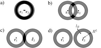
Before turning to detailed calculations, we wish to give some general physical interpretation of this physical quantity. The basic idea is that important correlations are obtained whenever the two quantum cyclotron rings (associated to circular wave functions in a perpendicular magnetic field $B$) have a large spatial overlap (disorder plays, however, a crucial role in correlating locally the states, as we will see later on). Focusing first on the spatial dependence of $\chi(r,\omega_{1},\omega_{2})$ for equal tip voltages, one readily understands that the intersection of the quantum rings (with width of the order of magnetic length $l_{B}=\sqrt{\hbar c/|e|B}$) around the two tip positions provides an increased area of intersection [from $l_{B}^{2}$ to $l_{B}^{3/2}(R^{L})^{1/2}$] when the distance between the points is close to the sum of the Larmor radii $R^{L}$ (see Fig 1 and caption for details). This already suggests that a peak should occur in the LDoS-LDoS correlations for this particular distance. We note that this effect has no classical analog, as quantum cyclotron rings collapse into circular cyclotron orbits at vanishing $l_{B}$ (in fact, we will see that a kink instead of a peak occcurs in the classical limit). The energy dependence (given by the two tip voltages) can be also easily inferred, for instance, at coinciding tip positions. When both tip energies precisely match the Landau levels, maximal overlap of the whole quantum cyclotron rings occur, leading to sharp and large positive correlations. However, detuning the two tip energies will probe correlations between different circular wave functions, and destroy the correlations. In that case, the square averaged term in Eq. (1) will dominate the averaged square one, leading then to weak and negative correlations.

Figure 1: Geometric interpretation of correlations of the LDoS in terms of overlap of quantum cyclotron rings of width $l_{B}$. Panel a) taken for close intertip distance $|{\bf r}_{1}-{\bf r}_{2}|\ll 2R^{L}$ presents a nearly maximal overlap area of the order $l_{B}R^{L}$ (with $R^{L}$ the Larmor radius), hence maximal correlations. Panel b) taken in the intermediate situation $|{\bf r}_{1}-{\bf r}_{2}|\simeq R^{L}$ has a small overlap area $l_{B}^{2}$, thus relatively weak correlations. Panel c) taken at tangent cyclotron orbits $|{\bf r}_{1}-{\bf r}_{2}|\simeq 2R^{L}$ has a small increased overlap area of the order $l_{B}^{3/2}(R^{L})^{1/2}$ (for $R^{L}>l_{B}$), so that a moderate peak as a function of intertip distance occurs. Finally panel d) presents the situation of non-overlaping cyclotron orbits at $|{\bf r}_{1}-{\bf r}_{2}|\gg 2R^{L}$, hence exponentially suppressed LDoS-LDoS correlations.

The paper is organized as follows. Section II recalls the form of the local density of states (for fixed but smooth disorder) in quantum Hall systems Champel2009 . We consider, in turn, the disorder averaged LDoS in Sec. III, allowing us to present the technique on a simple and more usual quantity, and to test the approximation scheme. Then Sec. IV presents the derivation of the disorder averaged LDoS-LDoS correlations, which are finally discussed in great detail in Sec. V.

II Local density of states at high magnetic field

We now present our theoretical analysis of this problem, which can be carried out fully analytically for smooth disorder in the high magnetic field regime, and which confirms the above argumentation. The basic model is a single-particle Hamiltonian for an electron confined in two dimensions in the presence of both a perpendicular magnetic field ${\bf B}$ and an arbitrary potential energy $V({\bf r})$,

$$H=\frac{1}{2m^{\ast}}\left(-i\hbar{\bm{\nabla}}_{{\bf r}}-\frac{e}{c}{\bf A}({\bf r})\right)^{2}+V({\bf r}),$$ (2)

with the vector potential ${\bf A}$ such that ${\bm{\nabla}}\times{\bf A}={\bf B}=B\hat{{\bf z}}$, and $m^{\ast}$ the electron effective mass [here ${\bf r}=(x,y)$ is the position of the electron in the plane]. We do not consider the case of graphene here, which can be easily extended following our previous results Champel2010 , although this system is quite relevant experimentally for the considerations of the present work.

The starting point is the realistic assumption of large cyclotron frequency (compared to local amplitude fluctuations of the disordered potential) at large magnetic field, so that Landau level mixing can be disregarded and the guiding center coordinate ${\bf R}$ follows a quantum motion along weakly curved equipotential lines. In that case the guiding center Green’s function obeys a single pole structure for each Landau level $n$ as found in Refs. Champel2009, and Champel2010, [this generalizes the results of Ref. Raikh1995, to arbitrary Landau levels]:

$$G_{n}({\bf R}) = \frac{1}{\omega-E_{n}-V_{n}({\bf R})+i0^{+}}$$ (3)

where $E_{n}=\hbar\omega_{c}(n+1/2)$ are the Landau level energies and $\omega_{c}=|e|B/(m^{\ast}c)$ is the cyclotron frequency. One important quantity above is the effective potential $V_{n}({\bf R})$ that results from averaging the bare disorder potential $V({\bf R})$ along the quantum cyclotron motion

$$V_{n}({\bf R})=\int d^{2}{\bm{\eta}}\;F_{n}({\bf R}-{\bm{\eta}})V({\bm{\eta}}).$$ (4)

The kernel $F_{n}({\bf R})$ here is given by the following expression Champel2009 :

$$F_{n}({\bf R})=\frac{1}{\pi n!l_{B}^{2}}\frac{\partial^{n}}{\partial s^{n}}\left.\frac{e^{-A_{s}{\bf R}^{2}/l_{B}^{2}}}{1+s}\right|_{s=0}$$ (5)

with $A_{s}=(1-s)/(1+s)$, and can also be written in an equivalent form note1

$$F_{n}({\bf R})=\frac{(-1)^{n}}{\pi l_{B}^{2}}L_{n}\left(\frac{2{\bf R}^{2}}{l_{B}^{2}}\right)e^{-{\bf R}^{2}/l_{B}^{2}},$$ (6)

where $L_{n}(z)$ is the Laguerre polynomial of degree $n$. This kernel is also known as the form factor in the literature on quantum Hall effects form . Expression (5) turns out to be very useful for the study of the first several Landau levels, while expression (6) is more suited for the consideration of high Landau levels ($n\gg 1$). Apart from the case $n=0$, we note that the kernel $F_{n}({\bf R})$ is not a positive-definite function, and cannot be interpreted as a wave function probability density. Instead, it rather corresponds to a Wigner distribution because the physical space of the guiding center coordinates ${\bf R}=(X,Y)$ is, in fact, associated to a pair of conjugate variables owing to the commutation relation $[\hat{X},\hat{Y}]=il_{B}^{2}$ in the operatorial language. However, integration of the kernel $F_{n}({\bf R})$ over an arbitrary line provides a translationally invariant Landau states probability density. In the classical limit $n\to\infty$, while keeping the (Larmor) cyclotron radius $R^{L}_{n}=\sqrt{2n}l_{B}$ finite (hence for $l_{B}\rightarrow 0$), one gets note2 $F_{n}({\bf R})\simeq\frac{1}{2\pi R^{L}_{n}}\delta(|{\bf R}|-R^{L}_{n})$, so that the effective potential Eq. (4) corresponds to an average over the classical cyclotron orbit, as previously shown in Ref. Raikh1993, . For a nonzero $l_{B}$, $F_{n}({\bf R})$ is an oscillating function that shows a sharp peak of width $l_{B}$ centered around $|{\bf R}|\simeq R^{L}_{n}$. This quantity will be a crucial ingredient later on for the mathematical identification of the quantum cyclotron rings.

Finally, the LDoS is readily connected Champel2009 ; Champel2010 to the guiding center Green’s function given in Eq. (3)

$$\rho({\bf r},\omega)=\int\frac{d^{2}{\bf R}}{2\pi l_{B}^{2}}\sum_{n=0}^{+\infty}F_{n}({\bf R}-{\bf r})\frac{-1}{\pi}\mathrm{Im}\,G_{n}({\bf R},\omega).$$ (7)

Here one did not include the overall spin degeneracy. In practice, the signal measured by local scanning tunneling spectroscopy is directly related to the local density of states through an energy convolution with the derivative of the Fermi-Dirac distribution and the experimental resolution window. Apart from the condition of high cyclotron energy, the present calculation is valid for smooth potentials at the scale of $l_{B}$. Such a restriction on the spatial variations of the potential is, in fact, not very drastic because the above results are exact for arbitrary one-dimensional (1D) potentials Champel2009 (even very rough ones). For the realistic two-dimensional (2D) potential the validity of the calculation is controlled by the small energy scale associated typically to potential curvature Champel2009

$$E_{\mathrm{curvature}}=\frac{l_{B}^{2}}{2}\sqrt{|\partial_{XX}V_{n}\partial_{YY}V_{n}-(\partial_{XY}V_{n})^{2}|}.$$ (8)

A more precise evaluation of the degree of reliability of our approximation scheme for rough potentials will be given at the end of the next section. Before considering the correlations of the LDoS, we compute now in some detail the disorder averaged LDoS itself.

III Disorder averaged LDoS at high magnetic field

We first examine the disorder averaged LDoS, obtained experimentally by spatially sampling the STS current over a single STM tip position. Theoretically, the averaging procedure of expression (7) will be carried through an isotropic distribution function $\tilde{C}(q)$ in Fourier space (here $q=|{\bf q}|$) that describes the spatial correlations of disorder

$$\left<V({\bf R}_{1})V({\bf R}_{2})\right> = C({\bf R}_{1}-{\bf R}_{2})$$

$$= \int\frac{d^{2}{\bf q}}{(2\pi)^{2}}\tilde{C}(q)\,e^{-i{\bf q}\cdot({\bf R}_{1}-{\bf R}_{2})}.$$

Typically one can take $C({\bf R})=v^{2}e^{-|{\bf R}|^{2}/\xi^{2}}$, defining the correlation length $\xi$ and the root mean square value $v=\sqrt{\left<V({\bf R})^{2}\right>}$ of the bare disorder distribution. In that case $\tilde{C}(q)=\pi v^{2}\xi^{2}e^{-\xi^{2}q^{2}/4}$. Averaging of the LDoS (7) then simply follows from exponentiating the single pole in Eq. (3) by going in the time domain, and performing Gaussian integration over all possible disorder realizations

$$\left<\rho({\bf r},\omega)\right> = \int\!\!\!\frac{dt}{2\pi}\int\!\!\!\frac{d^{2}{\bf R}}{2\pi l_{B}^{2}}\sum_{n=0}^{+\infty}F_{n}({\bf R}-{\bf r})\int\!\!\!\mathcal{D}V\,$$

$$\times\exp\left\{i[\omega-E_{n}-V_{n}({\bf R})]t-\frac{1}{2}\int\frac{d^{2}{\bf q}}{(2\pi)^{2}}\frac{|\tilde{V}({\bf q})|^{2}}{\tilde{C}(q)}\right\}.$$

The effective potential Eq. (4) is given in Fourier space by $\tilde{V}_{n}({\bf q})=\tilde{F}_{n}(q)\tilde{V}({\bf q})$, where $\tilde{F}_{n}(q)$ is the Fourier transform of kernel (5), which is easily shown to obey

$$\tilde{F}_{n}(q) = \int d^{2}{\bf r}\,e^{i{\bf q}.{\bf r}}F_{n}({\bf r})=\frac{1}{n!}\frac{\partial^{n}}{\partial s^{n}}\left.\frac{e^{-l_{B}^{2}q^{2}/(4A_{s})}}{(1+s)A_{s}}\right|_{s=0}$$ (11)

$$= (-1)^{n}\pi l_{B}^{2}\,F_{n}(l_{B}^{2}{\bf q}/2).$$

One can then readily perform the functional integral over the disorder realizations in Eq. (III):

$$\left<\rho({\bf r},\omega)\right> = \int\!\!\!\frac{dt}{2\pi}\int\!\!\!\frac{d^{2}{\bf R}}{2\pi l_{B}^{2}}\sum_{n=0}^{+\infty}e^{i(\omega-E_{n})t}F_{n}({\bf R}-{\bf r})$$ (12)

$$\times\exp\left\{-\frac{1}{4}t^{2}\,\Gamma_{n}^{2}\right\}$$

where the energy width $\Gamma_{n}$ is given by the relation

$$\Gamma_{n}^{2}=2\int\!\!\!\frac{d^{2}{\bf q}}{(2\pi)^{2}}\tilde{C}(q)\left|\tilde{F}_{n}(q)\right|^{2}.$$ (13)

This result was obtained initially in Ref. Champel2010, for the case of graphene.

Expression (12) for the averaged density of states (DoS) is obviously ${\bf r}$ independent, so that the ${\bf R}$ integral can be carried using the normalization condition $\int d^{2}{\bf R}\,F_{n}({\bf R})=1$. The remaining time integral gives the final result

$$\left<\rho({\bf r},\omega)\right>=\frac{1}{2\pi l_{B}^{2}}\sum_{n=0}^{+\infty}\frac{1}{\sqrt{\pi}\Gamma_{n}}\exp\left\{-\left(\frac{\omega-E_{n}}{\Gamma_{n}}\right)^{2}\right\},$$ (14)

which takes the expected Gaussian lineshape.

The renormalized disorder width $\Gamma_{n}$ given in Eq. (13) can be analyzed note2 in the classical limit $n\rightarrow+\infty$, keeping the cyclotron radius $R^{L}_{n}=\sqrt{2n}l_{B}$ fixed and $l_{B}\to 0$. In this regime, we recover results first derived in Ref. Raikh1993 using a completely unrelated method

$$\Gamma_{n}=\sqrt{\int\frac{qdq}{2\pi}2\tilde{C}(q)[J_{0}(R^{L}_{n}q)]^{2}},$$ (15)

with $J_{0}(z)$ the zeroth order Bessel function. For very large classical orbits such that $R_{n}^{L}\gg\xi$, the large-argument asymptotics of the zeroth order Bessel function $J_{0}(z)\simeq\sqrt{2/(\pi z)}\cos(z-\pi/4)$ can be used, so that

$$\Gamma_{n}\simeq\sqrt{\frac{\int dq\,2\tilde{C}(q)}{\pi^{2}R^{L}_{n}}}\propto\frac{1}{n^{1/4}},$$ (16)

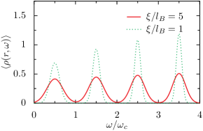
showing a decrease of the Landau level energy width with increasing index $n$. We note that expression (13) is more general than the classical result (15) because it incorporates wave function spreads on the scale $l_{B}$, a purely quantum lengthscale which has completely disappeared in the classical limit. In all cases (classical or quantum), the general trend is that the cyclotron motion averages out the local potential at increasing radius $R^{L}_{n}$, so that the energy width of the sample averaged DoS decreases with $n$. This effect is clearly seen Hashi2008 ; Miller2009 ; Miller2010 from the experimentally measured spatial dispersion of the LDoS, which shows a rapid narrowing for higher Landau levels. However, in the opposite limit of very smooth disorder $\xi\gg R^{L}_{n}$, this averaging by the cyclotron orbits becomes less efficient, and the energy width $\Gamma_{n}$ depends very weakly on the Landau level index $n$. Both regimes are presented in Fig. 2 showing the energy-dependent disorder averaged density of states for two values of $\xi/l_{B}$.

Figure 2: (color online) Disorder averaged density of states [in units of $(2\pi l_{B}^{2}v)^{-1}$] as a function of energy for two values of the correlation length of the disorder distribution ($\xi/l_{B}=5$ and $\xi/l_{B}=1$) spanning the first four Landau levels.

We end up by commenting on the reliability of our calculations for realistic disorders, and possibly rough ones at the scale of $l_{B}$. From the construction of the quantum guiding center theory Raikh1995 ; Champel2009 as a systematic gradient expansion, the lowest order calculations used here become exact for smooth disorder, namely $\xi\gg l_{B}$. In the opposite limit $\xi\ll l_{B}$, the approximation scheme does not fully break down per se, thanks to the wave function averaging on the scale $l_{B}$ performed within the effective potential (4). This implies that the effective potential varies on the scale $\sqrt{\xi^{2}+l_{B}^{2}}$ and remains smooth even for very rough bare potential ($\xi\ll l_{B}$). In this regime, the theory simply misses then the small parameter $l_{B}^{2}/(\xi^{2}+l_{B}^{2})$ of the case $\xi\gg l_{B}$, and its adequation becomes purely a quantitative matter. Interestingly, we are able to assess its validity thanks to Wegner’s exact solution Wegner for the disorder averaged density of states in the Landau level $n=0$, calculated for $\delta$-correlated disorder $\left<V({\bf R})V({\bf 0})\right>=w\,\delta^{(2)}({\bf R})$

$$\left<\rho({\bf r},\omega)\right>_{\mathrm{exact}}=\frac{1}{2\pi l_{B}^{2}}\frac{2^{3/2}}{\pi^{3/2}\Gamma_{0}}\frac{\exp[2(\omega-E_{0})^{2}/\Gamma_{0}^{2}]}{1+\{\mathrm{Erfi}[\sqrt{2}(\omega-E_{0})/\Gamma_{0})]\}^{2}}$$

(17)

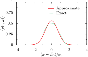
In the previous formula, $\mathrm{Erfi}(x)=2\pi^{-1/2}\int_{0}^{x}\mathrm{d}u\,e^{u^{2}}$ is the so-called complex error function and $\Gamma_{0}^{2}=w/(\pi l_{B}^{2})$. In our calculation, the $\delta$-correlated potential is obtained from the $\xi\rightarrow 0$ limit in Eq. (III), which corresponds to the most stringent limit to test our approximation scheme. The comparison (derived for the same microscopic disorder parameters) between the Gaussian expression (14) in the lowest Landau level $n=0$, using the linewidth (13), with Wegner’s exact formula Wegner , written in Eq. (17), is given in Fig. 3. Although neither the peak value nor the tails (not shown) are exactly reproduced within our approximation, the result is close to the exact answer, and this is surprising because we are far from the naive domain of validity of the theory.

Figure 3: (color online) Comparison of the disorder averaged density of states [in units of $(2\pi l_{B}^{2}\Gamma_{0})^{-1}$] in the Landau level $n=0$ between Wegner’s exact formula and our leading order gradient approximation for the extreme case of $\delta$-correlated disorder ($\xi/l_{B}=0$). Rapid convergence of the approximation scheme is expected as soon as $\xi\gtrsim l_{B}$.

This comparison gives some evidence that both the disorder averaged LDoS and its nonlocal correlations (to be calculated now), will be quantitatively obtained by a gradient expansion in the disorder for realistic cases where $\xi\gtrsim l_{B}$ (granted by the high magnetic field limit). Moreover, we stress that Wegner’s method does not apply to obtain two-particle averages, and cannot be used to calculate the LDoS-LDoS correlations, showing the greater generality of our approach.

IV Disorder averaged LDoS-LDoS correlations at high magnetic field

We are now ready to calculate the two-point correlations of the LDoS, taken at two different tip positions ${\bf r}_{1},{\bf r}_{2}$ and for two different energies $\omega_{1}$, $\omega_{2}$. The starting point is the expression

$$\!\!\left<\rho({\bf r}_{1},\omega_{1})\rho({\bf r}_{2},\omega_{2})\right>\!\!\! = \!\!\!\int\!\!\!\frac{dt_{1}}{2\pi}\!\!\int\!\!\!\frac{dt_{2}}{2\pi}\!\!\int\!\!\!\frac{d^{2}{\bf R}_{1}}{2\pi l_{B}^{2}}\!\!\int\!\!\!\frac{d^{2}{\bf R}_{2}}{2\pi l_{B}^{2}}\!\!\sum_{n_{1}=0}^{+\infty}\sum_{n_{2}=0}^{+\infty}$$ (18)

$$\times F_{n_{1}}({\bf R}_{1}-{\bf r}_{1})F_{n_{2}}({\bf R}_{2}-{\bf r}_{2})e^{i(\omega_{1}-E_{n_{1}})t_{1}+i(\omega_{2}-E_{n_{2}})t_{2}}$$

$$\times A({\bf R}_{1},n_{1},t_{1};{\bf R}_{2},n_{2},t_{2})$$

where the following disorder average must be performed:

$$A({\bf R}_{1},n_{1},t_{2};{\bf R}_{2},n_{2},t_{2})\!\! = \!\!\int\!\!\!\mathcal{D}V\,e^{-i[V_{n_{1}}({\bf R}_{1})t_{1}+V_{n_{2}}({\bf R}_{2})t_{2}]}$$

$$\times\exp\left\{-\frac{1}{2}\int\frac{d^{2}{\bf q}}{(2\pi)^{2}}\frac{|\tilde{V}({\bf q})|^{2}}{\tilde{C}(q)}\right\}$$

$$=\exp\left\{-\frac{1}{2}\int\!\!\!\frac{d^{2}{\bf q}}{(2\pi)^{2}}\tilde{C}(q)\Big{|}\sum_{i=1,2}t_{i}\tilde{F}_{n_{i}}(q)e^{i{\bf q}.{\bf R}_{i}}\Big{|}^{2}\right\}$$

$$=\exp\left\{-\frac{1}{4}\left[t_{1}^{2}\Gamma_{n_{1}}^{2}+t_{2}^{2}\Gamma_{n_{2}}^{2}+2t_{1}t_{2}S_{n_{1},n_{2}}({\bf R}_{1}-{\bf R}_{2})\right]\right\}.$$

The energy width $\Gamma_{n}$ was already defined in Eq. (13), and a spatially dependent disorder correlator now appears

$$\!\!\!S_{n_{1},n_{2}}({\bf R})=2\int\!\!\!\frac{d^{2}{\bf q}}{(2\pi)^{2}}\tilde{C}(q)\tilde{F}_{n_{1}}(q)\tilde{F}_{n_{2}}(q)\cos({\bf q}\cdot{\bf R}).$$ (19)

Using expressions (5) and (11), we can perform exactly the integrals in Eq. (19) and find a result which can be written under the form

$$\!\!\!S_{n_{1},n_{2}}(R)=\frac{2v_{0}^{2}}{n_{1}!n_{2}!}\frac{\partial^{n_{1}+n_{2}}}{\partial s_{1}^{n_{1}}\partial s_{2}^{n_{2}}}\Bigg{[}(1-s_{1}-s_{2}+s_{1}s_{2})^{-1}$$

$$\times\frac{\xi^{2}}{\xi^{2}+2B_{s_{1},s_{2}}l_{B}^{2}}\exp\left(-\frac{R^{2}}{\xi^{2}+2B_{s_{1},s_{2}}l_{B}^{2}}\right)\Bigg{]}_{s_{1}=s_{2}=0},$$ (20)

where we have introduced the short-hand notation

$$B_{s_{1},s_{2}}=\frac{1-s_{1}s_{2}}{1-s_{1}-s_{2}+s_{1}s_{2}}.$$ (21)

Note that the disorder correlator $S_{n_{1},n_{2}}(R)$ is isotropic (i.e., only depends on the distance $R=|{\bf R}|$). In addition, its diagonal elements taken at $R=0$ are related to the energy width $\Gamma_{n}$ via the relation $S_{n,n}(0)=\Gamma_{n}^{2}$. For a smooth disordered potential such that $\xi\gg l_{B}$, we can easily check from Eq. (20) that the functions $S_{n_{1},n_{2}}(R)$ are peaked at $R=0$ and decay in a Gaussian way with a characteristic length scale given by $\xi$ for the first few Landau levels. For higher Landau levels, the disorder correlator $S_{n_{1},n_{2}}(R)$ spreads over a bigger characteristic distance. For instance, for $n_{1}=n_{2}=n\gg 1$, it has an extent of the order of $\sqrt{(R^{L}_{n})^{2}+\xi^{2}}$.

Shifting the space integrals in Eq. (18), we see that the quantity $\left<\rho({\bf r}_{1},\omega_{1})\rho({\bf r}_{2},\omega_{2})\right>$ is clearly described by a function of ${\bf r}={\bf r}_{1}-{\bf r}_{2}$ only. In the following we will consider the centered two-point correlator of the LDoS defined in Eq. (1). Integration over the time variables in Eq. (18) can be performed analytically and yields the expression for the LDoS-LDoS correlator

$$\chi({\bf r},\omega_{1},\omega_{2})=\int\!\!\!\frac{d^{2}{\bf R}_{1}}{2\pi l_{B}^{2}}\!\!\int\!\!\!\frac{d^{2}{\bf R}_{2}}{2\pi l_{B}^{2}}\!\!\sum_{n_{1}=0}^{+\infty}\sum_{n_{2}=0}^{+\infty}\!\!F_{n_{1}}({\bf R}_{1}-{\bf r}_{1})$$

$$\times F_{n_{2}}({\bf R}_{2}-{\bf r}_{2})\,\Theta_{n_{1},n_{2}}\left(\left|{\bf R}_{1}-{\bf R}_{2}\right|,\omega_{1},\omega_{2}\right)\hskip 17.07182pt$$ (22)

with

$$\Theta_{n_{1},n_{2}}\left(R,\omega_{1},\omega_{2}\right)=\frac{1}{\pi}\left\{\left[\Gamma_{n_{1}}^{2}\Gamma_{n_{2}}^{2}-[S_{n_{1},n_{2}}(R)]^{2}\right]^{-1/2}\right.$$

$$\times e^{-\frac{(\omega_{1}-E_{n_{1}})^{2}\Gamma_{n_{2}}^{2}+(\omega_{2}-E_{n_{2}})^{2}\Gamma_{n_{1}}^{2}-2(\omega_{1}-E_{n_{1}})(\omega_{2}-E_{n_{2}})S_{n_{1},n_{2}}(R)}{\Gamma_{n_{1}}^{2}\Gamma_{n_{2}}^{2}-[S_{n_{1},n_{2}}(R)]^{2}}}$$

$$-\left[\Gamma_{n_{1}}\Gamma_{n_{2}}\right]^{-1}e^{-\frac{(\omega_{1}-E_{n_{1}})^{2}}{\Gamma^{2}_{n_{1}}}}e^{-\frac{(\omega_{2}-E_{n_{2}})^{2}}{\Gamma^{2}_{n_{2}}}}\left.\frac{}{}\right\}.\hskip 14.22636pt$$ (23)

Although the above expressions are still too complicated to make precise statements on the nature of the LDoS-LDoS correlations, we can already infer some of the early predictions formulated in the Introduction. Clearly the two kernels $F_{n}({\bf R-r})$ in Eq. (22) centered on the two positions of the tip ${\bf r}_{1}$ and ${\bf r}_{2}$ impose a constraint on the two guiding center coordinates ${\bf R}_{1}$ and ${\bf R}_{2}$, which must live predominantly within cyclotron rings of extent $R^{L}_{n_{1}}$ and $R^{L}_{n_{2}}$ with width $l_{B}$ (we note that the kernels have rather $n$ oscillations within a given radius $R^{L}_{n}$, so that there are in total $n$ different rings for a given quantum state). This formula thus confirms our initial expectation that the area of overlap between two cyclotron rings dictates the behavior of the LDoS-LDoS correlations. A second interesting aspect is that it is the additional disorder-dependent kernel $\Theta_{n_{1},n_{2}}$ which permits nontrivial correlations. Should this complicated function of energy and space be negligible, one would end up with vanishing correlations.

Yet, to get more quantitative understanding of the complete integral in Eq. (22), one needs to further simplify the above expressions. This can be achieved by introducing the change in variables ${\bf R}^{\prime}=({\bf R}_{1}+{\bf R}_{2})/2$ and ${\bf R}={\bf R}_{2}-{\bf R}_{1}$. After integration over the center-of-mass position ${\bf R}^{\prime}$, we get

$$\chi({\bf r},\omega_{1},\omega_{2})=\sum_{n_{1}=0}^{+\infty}\sum_{n_{2}=0}^{+\infty}\int\!\!\!\frac{d^{2}{\bf R}}{2\pi l_{B}^{2}}f_{n_{1},n_{2}}({\bf R}+{\bf r})$$

$$\times\Theta_{n_{1},n_{2}}\left(R,\omega_{1},\omega_{2}\right)$$ (24)

with

$$f_{n_{1},n_{2}}({\bf R})=\int\!\!\!\frac{d^{2}{\bf R}^{\prime}}{2\pi l_{B}^{2}}F_{n_{1}}\left({\bf R}^{\prime}-\frac{{\bf R}}{2}\right)F_{n_{2}}\left({\bf R}^{\prime}+\frac{{\bf R}}{2}\right)$$

$$=\frac{(2\pi l_{B}^{2})^{-2}}{n_{1}!n_{2}!}\left.\frac{\partial^{n_{1}+n_{2}}}{\partial s_{1}^{n_{1}}\partial s_{2}^{n_{2}}}\frac{\exp\left(-{\bf R}^{2}/\left[2l_{B}^{2}B_{s_{1},s_{2}}\right]\right)}{1-s_{1}s_{2}}\right|_{s_{1}=s_{2}=0},$$ (25)

where we have used expression (5) for the kernel $F_{n}({\bf R})$. Then, introducing the polar coordinates for the position ${\bf R}$ and performing the angular integral in Eq. (24), we arrive at the final expression of the disorder averaged LDoS-LDoS correlations (which now obviously is only function of the intertip distance $r=|{\bf r}|$):

$$\chi(r,\omega_{1},\omega_{2})=\sum_{n_{1}=0}^{+\infty}\sum_{n_{2}=0}^{+\infty}l_{B}^{-2}\int_{0}^{+\infty}\!\!\!\!\!\!\!RdR\,h_{n_{1},n_{2}}(R,r)$$

$$\times\Theta_{n_{1},n_{2}}\left(R,\omega_{1},\omega_{2}\right),$$ (26)

where

$$h_{n_{1},n_{2}}(R,r)=\int_{0}^{2\pi}\!\!\frac{d\theta}{2\pi}\,f_{n_{1},n_{2}}\left(\sqrt{R^{2}+r^{2}+2rR\cos\theta}\right)$$

$$=\frac{(2\pi l_{B}^{2})^{-2}}{n_{1}!n_{2}!}\frac{\partial^{n_{1}+n_{2}}}{\partial s_{1}^{n_{1}}\partial s_{2}^{n_{2}}}\,\Bigg{[}I_{0}\left(\frac{rR}{l_{B}^{2}B_{s_{1},s_{2}}}\right)\hskip 17.07182pt$$

$$\times\frac{\exp\left(-\left[{\bf R}^{2}+{\bf r}^{2}\right]/\left[2l_{B}^{2}B_{s_{1},s_{2}}\right]\right)}{1-s_{1}s_{2}}\Bigg{]}_{s_{1}=s_{2}=0}\hskip 14.22636pt$$ (27)

with $I_{0}(x)$ the modified Bessel function of the first kind. An alternative writing of Eq. (27) obtained by going to the Fourier space, which turns out to be more suitable for the consideration of large $n_{1}$ and $n_{2}$, is as follows:

$$h_{n_{1},n_{2}}(R,r)=\frac{l_{B}^{2}}{\left(2\pi l_{B}^{2}\right)^{2}}\int_{0}^{+\infty}\!\!\!\!\!\!\!\!dq\,q\tilde{F}_{n_{1}}(q)\tilde{F}_{n_{2}}(q)J_{0}(Rq)$$

$$\times J_{0}(rq).$$ (28)

The above expressions (26) through (28) are exact for arbitrary 2D smooth disorder (i.e., $\xi\gg l_{B}$).

V Discussion of the LDoS-LDoS correlations

V.1 Spatial dependence of the correlations

Let us now analyze the LDoS-LDoS correlations on the basis of Eq. (26). We see that the correlations result from the combination of two functions $h_{n_{1},n_{2}}(R,r)$ and $\Theta_{n_{1},n_{2}}\left(R,\omega_{1},\omega_{2}\right)$, which are quite different in nature. Obviously, only the functions $\Theta_{n_{1},n_{2}}\left(R,\omega_{1},\omega_{2}\right)$ defined in Eq. (23) contain the information about the energy dependence. For sufficiently widely separated Landau levels, the overlap between two states with two given energies $\omega_{1}$ and $\omega_{2}$ vanishes for most of the Landau level pairs due to the sharp energy Gaussians cutoff in Eq. (23), so that essentially only the one specific pair of Landau levels $(n_{1},n_{2})$ that is associated to the cyclotron energies $(E_{n_{1}},E_{n_{2}})$ closest to the tip voltages $(\omega_{1},\omega_{2})$ yields a nonzero contribution in the sum over Landau levels indices in Eq. (26). Furthermore, the LDoS-LDoS correlator $\chi(r,\omega_{1},\omega_{2})$ clearly vanishes whenever the disorder correlator $S_{n_{1},n_{2}}(R)$ is small compared to $\Gamma_{n_{1}}\Gamma_{n_{2}}$ due to the exact cancellation by the square averaged term in Eq. (23). Therefore, the main contributions to the correlations arise when $S_{n_{1},n_{2}}(R)\sim\Gamma_{n_{1}}\Gamma_{n_{2}}$.

In contrast, the functions $h_{n_{1},n_{2}}(R,r)$ are independent of the characteristic features of the disorder and have a pure geometric origin (as already discussed, they contain information on the spatial overlap of the quantum cyclotron rings). For $r=0$, we have the relation $h_{n_{1},n_{2}}(R,0)=f_{n_{1},n_{2}}({\bf R})$ from which a simple physical interpretation can be easily drawn. Using the semiclassical physical picture of the kernel $F_{n}({\bf R})$ put forward previously, we understand that nonzero contributions for $f_{n_{1},n_{2}}({\bf R})$ in Eq. (IV) are picked up only from the (quantum broadened on scale $l_{B}$) cyclotron orbits with radii $R^{L}_{n_{1}}$ and $R^{L}_{n_{2}}$ that live around the points $\pm{\bf R}/2$ separated by the distance $R$. This statement can be proved on more mathematical grounds starting from expression (28). Taking the limits $n_{1}$ and $n_{2}\to\infty$ in Eq. (28) as done in Ref. note2, , we obtain an approximate formula, which reads

$$h_{n_{1},n_{2}}(R,r)\simeq\frac{l_{B}^{2}}{\left(2\pi l_{B}^{2}\right)^{2}}\int_{0}^{+\infty}\!\!\!\!\!\!\!\!dq\,qJ_{0}(R^{L}_{n_{1}}q)\,J_{0}(R^{L}_{n_{2}}q)$$

$$\times J_{0}(Rq)\,J_{0}(rq).$$ (29)

For $r=0$, integral (29) strictly vanishes when $R>R^{L}_{n_{1}}+R^{L}_{n_{2}}$ or $R<\left|R^{L}_{n_{1}}-R^{L}_{n_{2}}\right|$. In the more realistic case of finite $n_{1}$ and $n_{2}$, this semiclassical limit shows that the resulting overlap of two quantum orbital motions turns out to be significant under the inequalities $\left|R^{L}_{n_{1}}-R^{L}_{n_{2}}\right|<R<R^{L}_{n_{1}}+R^{L}_{n_{2}}$. The functions $h_{n_{1},n_{2}}(R,r)$ being symmetrical in $R$ and $r$, we understand that for $R=0$ the contributions to the LDoS-LDoS correlations arise when the distance $r$ between the two tip positions is such that $\left|R^{L}_{n_{1}}-R^{L}_{n_{2}}\right|<r<R^{L}_{n_{1}}+R^{L}_{n_{2}}$, precisely as anticipated in the discussion of Fig. 1.

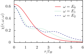
The spatial dependence of the two-point correlator $\chi(r,\omega_{1},\omega_{2})$ resulting from the numerical computation of the integral over the distance $R$ in Eq. (26) is shown in Fig. 4 in the regime of widely separated Landau peaks (we have taken in what follows $\hbar\omega_{c}=5\,v$). In these two figures, we have chosen the situation where the LDoS-LDoS correlations are maximal, that is, we have considered that the energies $\omega_{i}$ (here $i=1,2$) correspond exactly to Landau level energies $E_{n_{i}}$. The case of equal energies $\omega_{1}=\omega_{2}=\omega$ is first investigated in Fig. 4. According to the previous discussion, the dominant contributions among the different possible pairs of Landau level indices are the diagonal ones corresponding to $n_{1}=n_{2}=n$. For the lowest Landau level energy ($n=0$) shown with the solid line in Fig. 4, the correlations decrease in a monotonic way as a function of the distance $r$ between the two tip positions with a characteristic decay length of the order of the disorder correlation length $\xi$ (here all the distances are expressed in units of the magnetic length $l_{B}$ and we have taken $\xi=5\,l_{B}$). When the energy of the first Landau level is probed (dotted line of Fig. 4 corresponding to $\omega=E_{1}$), the spatial dependence of the correlations is still decreasing with the same decay length $\xi$, but it now exhibits a mild peak for the position $r$ close to $2R^{L}_{n}=2\sqrt{2n}l_{B}\approx 2.8l_{B}$ for $n=1$, associated to the overlap of the quantum cyclotron rings for the $n=1$ Landau states. In the second Landau level (at $\omega=E_{2}$), besides the peak close to $2R^{L}_{n}=4l_{B}$ for $n=2$, an additional peak is clearly seen in the $r$ dependence of the LDoS-LDoS correlations, see dashed line in Fig. 4. This is because the wave functions for $n>1$ have $n$ zeros, hence additional rings of high probability density.

Figure 4: (color online) LDoS-LDoS correlations at equal energies ($\omega_{1}=\omega_{2}=\omega$) as a function of the tips distance $r$ (in units of $l_{B}$) for different energies $\omega$. Here the correlations are expressed in units of $(2\pi l_{B}^{2}v)^{-2}$ with the parameters $\hbar\omega_{c}/v=5$ and $l_{B}/\xi=0.2$. The spatial dependence of the correlations presents peaks whose number corresponds to the Landau level index of the probed energy (for instance, for $\omega=E_{2}$ two peaks are seen).

This nonmonotonic spatial dependence observed for equal energies was anticipated in the Introduction of the paper, and can be understood more quantitatively as follows. When the disorder potential is smooth on the scale of $l_{B}$ (i.e., $\xi\gg l_{B}$) the two functions involved in the integrand of Eq. (26) are, in fact, characterized by two very different characteristic length scales. Indeed, the function $h_{n_{1},n_{2}}(R,r)$ decays with $R$ on the typical length scale $R^{L}_{n}=\sqrt{2n}l_{B}$ which, for indices $n$ not too big, turns out to be much smaller than the characteristic length scale (of the order of $\sqrt{(R^{L}_{n})^{2}+\xi^{2}}$) for the spatial variations of the functions $\Theta_{n,n}\left(R,\omega,\omega\right)$. Therefore, within the first few Landau levels a good approximation to the integral (26) is provided by the Laplace’s method owing to the inequality $\xi\gg R_{n}^{L}$. Using the formula

$$\int_{0}^{+\infty}\!\!\!dx\,I_{0}(ax)e^{-bx^{2}}=\sqrt{\frac{\pi}{4b}}e^{\frac{a^{2}}{8b}}I_{0}\left(\frac{a^{2}}{8b}\right),$$ (30)

we obtain the approximate analytical expression for the LDoS-LDoS correlations at identical tip energies ($\omega_{1}=\omega_{2}=\omega$) for $\omega$ close to the energy $E_{n}$

$$\chi(r,\omega,\omega)\simeq\frac{(2\pi l_{B}^{2})^{-2}}{2\pi v^{2}}\left\{\frac{\sqrt{\pi}\xi}{2\sqrt{2}l_{B}}e^{-(\omega-E_{n})^{2}/(2v^{2})}\frac{1}{(n!)^{2}}\frac{\partial^{2n}}{\partial s_{1}^{n}\partial s_{2}^{n}}\Bigg{[}\frac{\sqrt{B_{s_{1},s_{2}}}}{1-s_{1}s_{2}}I_{0}\left(\frac{r^{2}}{4l_{B}^{2}B_{s_{1},s_{2}}}\right)\,e^{-\frac{r^{2}}{4l_{B}^{2}B_{s_{1},s_{2}}}}\Bigg{]}_{s_{1}=s_{2}=0}-e^{-(\omega-E_{n})^{2}/v^{2}}\right\}.$$

(31)

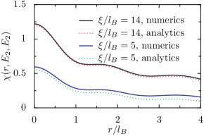
Consequently the nonmonotonous behavior of the correlations seen in Fig. 4 is connected with the oscillations of the function $h_{n,n}(0,r)$ within Eq. (26), and is fully described analytically by formula (31) in the regime $\xi\gg l_{B}$. As seen in Fig. 5 for two large values of $\xi/l_{B}$ and for energies taken at the second Landau level, the agreement between the numerical evaluation of the integral in Eq. (26) and the analytical approximation (31) is quite excellent.

Figure 5: (color online) LDoS-LDoS correlations at equal energies taken at the second Landau level ($\omega_{1}=\omega_{2}=E_{2}$) as a function of the tips distance $r$ (in units of $l_{B}$) for two different values of the disorder correlation length $\xi/l_{B}=14$ and $\xi/l_{B}=5$, with a comparison of the numerical evaluation of expression (26) and the analytical formula (31).

We note also that the correlations disappear (for generic values of the frequency) in the clean limit $v\to 0$ despite the $v^{-2}$ prefactor due to the exponential terms in Eq. (31), while they become singular precisely at the Landau level frequency.

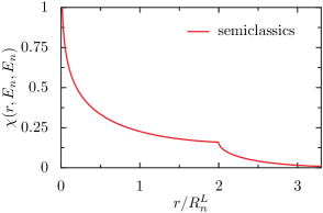
We would like to comment here on the semiclassical limit of fixed $R^{L}_{n}$ with $n\rightarrow\infty$ (and vanishing $l_{B}$) for the LDoS-LDoS correlations. In that case, we replace the kernel $F_{n}({\bf R})$ by $\frac{1}{2\pi R^{L}_{n}}\delta(|{\bf R}|-R_{n}^{L})$ in Eq. (22), and obtain numerically Fig. 6. Not surprisingly, the quantum oscillations at $r<2R_{n}^{L}$ disappear, yet a kink subsists for the exactly tangent cyclotron trajectories at $r=2R_{n}^{L}$, while a logarithmically diverging correlation occurs at $r=0$. These are classical remnants of the quantum effects discussed so far, and this robustness can again be expected according to the geometrical argument of Fig. 1 (now in the classical limit).

Figure 6: (color online) LDoS-LDoS correlations at equal energies taken at the Landau level ($\omega_{1}=\omega_{2}=E_{n}$) as a function of the tips distance $r$ (in units of $R^{L}_{n}$) in the semiclassical approximation ($l_{B}\to 0$) to integral (22).

These characteristic features can be understood analytically. Indeed, inserting Eq. (29) within formula (26), and performing Laplace’s method on the $R$-dependent integral (this is valid in the case $\xi\gg R^{L})$, we find

$$\chi(r,E_{n},E_{n})\simeq\frac{(2\pi l_{B}^{2})^{-2}}{2\pi v^{2}}\Bigg{(}\frac{\xi}{2}\int_{0}^{+\infty}\!\!\!\!\!\!\!\!dqJ_{0}(rq)[J_{0}(R^{L}q)]^{2}-1\Bigg{)}.$$ (32)

Expression (32) is clearly logarithmically divergent at $r=0$, but continuous at $r=2R^{L}$ (the situation of tangent cyclotron orbits). The spatial derivative of the correlator can be analyzed in the limit $r\to 2R^{L}$, and gives a finite derivative for $r<2R^{L}$ and a diverging one for $r>2R^{L}$, explaining the kink feature seen in Fig. 6. The onset of the logarithmic divergence at $r=0$ can be understood starting from the quantum expression (31), which alternatively reads for $r=0$ and $\omega=E_{n}$:

$$\chi(0,E_{n},E_{n})=\frac{(2\pi l_{B}^{2})^{-2}}{2\pi v^{2}}\Bigg{[}\frac{\xi}{\sqrt{2}l_{B}}\!\!\int_{0}^{+\infty}\!\!\!\!\!\!\!\!\!\!du\!\left[L_{n}\left(u^{2}\right)\right]^{2}\!e^{-u^{2}}\!\!-1\!\Bigg{]}.$$

The above equation is again obtained from Laplace’s method in the case $\xi\gg R_{n}^{L}$ to analytically perform the integral over $R$ in Eq. (22), and used the explicit expression (6) for the kernel $F_{n}$, instead of the derivative trick performed in Eq. (31). Using the asymptotic formula for the Laguerre polynomial in the large $n$ limit as in Ref. note2, , we get $\chi(0,E_{n},E_{n})\propto\log(n)/R_{n}^{L}$ with $R_{n}^{L}=\sqrt{2n}l_{B}$. We recover the logarithmic divergence for $n\to\infty$ and fixed $R_{n}^{L}$, while this expression vanishes as $\log(n)/\sqrt{n}$ for $n\to\infty$ and fixed $l_{B}$, in agreement with Fig. 4, where a slight decrease with increasing $n$ is seen at $r=0$. We thus stress that quantum mechanics (finite $l_{B}$) always regularizes the singular classical behavior, and that maximal correlations are, in fact, obtained (at a given magnetic field, hence fixed $l_{B}$) for the lowest Landau levels.

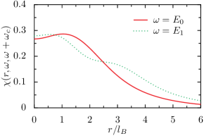
Let us come back to the quantum case of finite $l_{B}$ and investigate the effect of energy detuning in the spatial dependence of the LDoS correlator. For energies $\omega_{1}\neq\omega_{2}$ a different spatial structure from the situation of equal energies can be seen in Fig. 7, which corresponds to the cases $(\omega_{1},\omega_{2})=(E_{0},E_{1})$ and $(\omega_{1},\omega_{2})=(E_{1},E_{2})$, the solid and dotted lines, respectively. Unlike the equal energy cases of Fig. 4, the correlations are no more maximally obtained for the tips distance $r=0$ but for an intermediate tip distance of the order $|R^{L}_{1}-R^{L}_{2}|$, as can be guessed again from the geometrical interpretation of Fig. 1, in the case $R^{L}_{1}\neq R^{L}_{2}$. We note that the spatial dependence of the correlations between the first and second Landau levels is also characterized by an extra mild peak, a reminiscent feature of the equal energy case.

Figure 7: (color online) LDoS-LDoS correlations at unequal energies ($\omega_{1}=\omega$ and $\omega_{2}=\omega+\omega_{c}$) as a function of the tips distance $r$ (in units of $l_{B}$) for different energies $\omega$. We used the same parameters as in Fig. 4.

V.2 Energy dependence of the correlations

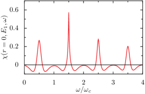
We now study the energy dependence of the LDoS-LDoS correlations. We have represented in Fig. 8 the correlator $\chi(r,\omega_{1},\omega_{2})$ as a function of the energy $\omega_{2}=\omega$ for identical tip positions (i.e., for $r=0$) when the first tip energy is pinned to the first Landau level ($\omega_{1}=E_{1}$).

Figure 8: (color online) LDoS-LDoS correlations for the tip distance $r=0$ and for the energy $\omega_{1}$ pinned to the first Landau level ($\omega_{1}=E_{1}$) as a function of the energy $\omega_{2}=\omega$. The other parameters are the same as in Fig. 4. The highest peak is obtained for $\omega_{2}=\omega_{1}$ and is accompanied by satellite peaks corresponding to the neighbouring energy levels of the first Landau level.

We note the presence of different peaks in the correlations corresponding to the sequence $\omega=E_{n}$ of the Landau levels energy peaks in the local density of states. However, it is worth noting that the LDoS-LDoS correlation peaks are much sharper than the LDoS peaks because of the sensitive matching of the spatial overlaps between the quantum rings associated to the states in Landau level $n_{1}=1$ and $n_{2}=n$. Besides the strongest peak obtained for $\omega=E_{1}$, a succession of lateral peaks occurs for all other cyclotron energies $E_{n}$, showing that nondiagonal elements of $h_{n_{1},n_{2}}(R,r)$ are also strongly correlated. More interestingly, the regions surrounding each of these sharp peaks with positive correlations are characterized by negative values for the correlator $\chi(0,E_{1},\omega_{2})$, thus corresponding to anticorrelations. This crossover from positive to negative correlations as a function of the energy can be easily understood on the basis of Eq. (23) at $\xi\gg R^{L}$, which is then well approximated by a small-$R$ expansion

$$\Theta_{n_{1},n_{2}}(R,\omega_{1},\omega_{2}) \simeq \frac{1}{2\pi v^{2}}\Bigg{(}\frac{\xi}{2R}e^{-\frac{\xi^{2}}{4R^{2}}\frac{(\omega_{1}-\omega_{2}+E_{n_{2}}-E_{n_{1}})^{2}}{2v^{2}}}$$ (34)

$$\times e^{-\frac{(\omega_{1}-E_{n_{1}})(\omega_{2}-E_{n_{2}})}{2v^{2}}}-e^{-\frac{(\omega_{1}-E_{n_{1}})^{2}+(\omega_{2}-E_{n_{2}})^{2}}{2v^{2}}}\Bigg{)}.$$

To obtain this expression, we have developed the disorder correlator $S_{n_{1},n_{2}}(R)$ [Eq. (19)] and the linewidth $\Gamma_{n}$ in the large $\xi$ limit. As can be seen in Eq. (34), a competition between two exponential terms occurs depending on the relative values of $\omega_{1}$ and $\omega_{2}$. For $\delta\omega\equiv\omega_{1}-\omega_{2}+E_{n_{2}}-E_{n_{1}}=0$, the first term in the right-hand side (r.h.s) of Eq. (34), which is large and positive (of the order of $\xi/R$), dominates over the second exponential contribution, and one gets positive LDoS-LDoS correlations, as already noted. For $\delta\omega$ slightly different from zero, the first term decreases exponentially fast (note the large $\xi^{2}/R^{2}$ prefactor within the exponential), resulting in the sharp peak observed in Fig. 8 near coinciding energies. At increasing $|\delta\omega|$, the second term in the r.h.s of Eq. (34), which has a small and negative amplitude, is characterized by a slower exponential decrease, and then gives the main contribution to the correlations. Coming back to the initial Eq. (1) for the correlator $\chi(r,\omega_{1},\omega_{2})$, we conclude that the square average density dominates quickly at increasing energy detuning.

Analytical insight can be obtained by further assuming the classical regime of $R^{L}\gg l_{B}$ (hence high Landau levels). Using then the approximation (29) within formula (26) together with Eq. (34) (which is valid in the limit $\xi\gg R^{L}$) we get the semiclassical approximation for the LDoS correlations at coinciding tip position $r=0$

$$\chi(0,\omega_{1},\omega_{2}) = \frac{\xi}{2\pi v^{2}(2\pi l_{B}^{2})^{2}}\sum_{n_{1},n_{2}}\int_{0}^{+\infty}\!\!\!\!\!\!\!\!\!dq\,qJ_{0}(R_{n_{1}}^{L}q)J_{0}(R_{n_{2}}^{L}q)\int_{0}^{+\infty}\!\!\!\!\!\!\!\!\!dR\,J_{0}(Rq)e^{-\frac{(\delta\omega)^{2}}{2v^{2}}\frac{\xi^{2}}{4R^{2}}}e^{-\frac{(\omega_{1}-E_{n_{1}})(\omega_{2}-E_{n_{2}})}{2v^{2}}}$$ (35)

$$-\big{<}\rho(0,\omega_{1})\big{>}\big{<}\rho(0,\omega_{2})\big{>}.$$

Here the double sum over $(n_{1},n_{2})$ is again constrained by the external frequencies $(\omega_{1},\omega_{2})$, and reduces to a single term in case of sharply defined LDoS-LDoS correlation peaks, giving rise to a single peak at $\omega_{1}-\omega_{2}=E_{n_{1}}-E_{n_{2}}$. Let us focus first on the case where $n_{1}=n_{2}$, so that $R_{n_{1}}^{L}=R_{n_{2}}^{L}=R^{L}$. We see that the above integrand in Eq. (35) then behaves as $1/q$ for vanishing $\delta\omega$, because $|J_{0}(R^{L}q)|^{2}$ looses its oscillatory character at large momentum $q$. One obtains thus a logarithmically diverging peak $\chi(0,\omega_{1},\omega_{2})\sim\log|v/\delta\omega|$, related to the $\log|l_{B}/r|$ spatial divergence found previously in the semiclassical limit at small intertip distance. However, for nonzero $n\equiv n_{1}-n_{2}$, the LDoS-LDoS correlation peak at $\omega_{1}-\omega_{2}=E_{n}$ is no more logarithmically diverging when $\delta\omega\to 0$. This is because the product $J_{0}(R_{n_{1}}^{L}q)J_{0}(R_{n_{2}}^{L}q)$ behaves as $\cos(l_{B}^{2}nq/R^{L})/q$ for large momentum $q$, as can be seen using the expression for the cyclotron radii $R_{n_{1,2}}^{L}=R^{L}\pm\frac{l_{B}^{2}n}{2R^{L}}$ in the limit $n\ll n_{1},n_{2}$, where $R^{L}\equiv\sqrt{n_{1}+n_{2}}l_{B}$. In order to capture the relevant energy scale at small $\delta\omega$, we can make the change in variables $k=(\xi|\delta\omega|/v)q$ and $z=(v/\xi\Omega_{n})R$ with $\Omega_{n}=nvl_{B}^{2}/(R^{L}\xi)$ into Eq. (35), and use the asymptotic form of the Bessel functions for $|\delta\omega|\ll\xi v/R^{L}$. After integration over $k$, this provides the deviation of the LDoS correlations from the $n^{\mathrm{th}}$ peak value (at $\delta\omega=0$)

$$\delta\chi=\frac{(2\pi l_{B}^{2})^{-2}}{2\pi^{2}v^{2}}\frac{\xi}{R^{L}}\int_{1}^{+\infty}\!\!\!\!dz\;\frac{e^{-\left|\frac{\delta\omega}{\Omega_{n}}\right|^{2}\frac{1}{8z^{2}}}-1}{\sqrt{z^{2}-1}}.$$ (36)

The new energy scale $\Omega_{n}$ therefore sets the width of the $n^{\mathrm{th}}$ correlation peak. Since $\Omega_{n}\ll v$ in the regime $\xi\gg R^{L}\gg l_{B}$, we recover the fact that the LDoS-LDoS correlations are more sharply defined than the average LDoS peaks. The linear increase of $\Omega_{n}$ with $n$ also explains the progressive smearing of the correlations at increasing energy detuning of the tips (see Fig. 8).

We now discuss the situation of strongly overlapping Landau level, $\omega_{c}\ll v=\sqrt{\left<V^{2}\right>}$, so that the average density of states becomes structureless. In that case, the sharper peaks in the LDoS-LDoS correlations can survive for smooth disorder ($\xi\gg l_{B}$), under the condition $vl_{B}/\xi\ll\omega_{c}$ for the lowest Landau levels. A similar result was already found by Rudin et al. Rudin , who studied the energy dependence of the local LDoS-LDoS correlations in a weak magnetic field and long classical orbits $R^{L}\gg\xi$ in the diffusive regime. The disorder dependence of correlator (31) in Ref. Rudin, was also in $1/v^{2}$ as in the present paper.

It is worth stressing that the condition to obtain sharp peaks in the LDoS-LDoS correlations corresponds precisely to the absence of local Landau level mixing. Indeed, transitions between adjacent Landau levels provide Champel2008 a typical energy scale $l_{B}^{2}|{\bm{\nabla}}V|^{2}/\omega_{c}$, so that our calculation is controlled when the parameter $(l_{B}^{2}/\xi^{2})(v^{2}/\omega_{c}^{2})$ is small. Clearly, large overlap in the average DoS can be compatible with no mixing, because this quantity relates to global properties (long-wavelength fluctuations) of the smooth disorder. In contrast, only the correlations of the LDoS can feel the local interplay of disorder and Landau quantization, and reveal whether the Landau index $n$ stays a good quantum number or not.

Interestingly, a logarithmic singularity for the $n=0$ peak and an energy width $\Omega_{n}$ proportional to $n^{2}$ for the $n^{\mathrm{th}}$ peak were obtained in the semiclassical diffusive regime Rudin . This is only slightly different from our results in the semiclassical limit, showing the continuity of the present physics from low to high magnetic fields. We emphasize again that quantum effects at finite magnetic length regularize the spurious divergences generically related to the semiclassical approximation.

Finally, we note that some of the energy-related features on the LDoS correlations discussed above have already been reported experimentally Konemann ; Holder in heavily doped three-dimensional (3D) GaAs semiconductors. For instance, conductance anticorrelations were observed Konemann in the presence of Landau levels, while the narrowing of the LDoS fluctuations has been found Holder at weak magnetic field. However, these experimental studies were performed using resonant tunneling impurity, hence at a fixed position, asking for a different analysis from what was performed here (besides the 3D character of the studied samples). Indeed, averaging was performed either over the applied voltage Holder or magnetic field Konemann , and in the later case, the Landau levels are simply lost. Spatial averaging in a STM configuration, as proposed in our work, should allow a greater control of the LDoS correlations (in terms of the applied magnetic field and tip voltages). Moreover, this offers a way to investigate spatial correlations of the LDoS, that could not be assessed with previous experimental techniques.

VI Conclusion

We have studied theoretically the two-point correlations of the local density of states in a disordered two-dimensional electron gas under a large magnetic field. A rich spatial dependence of the correlations was found, which can be qualitatively explained by geometrical overlaps of the two quantum cyclotron rings that roughly describe circular wave functions. The energy behavior of the correlations was shown to provide sharp peaks when the frequency detuning matches integer multiple of the cyclotron frequency, similar to the low magnetic field results of Rudin et al. Rudin . These sharp peaks in the LDoS correlations reveal that Landau levels correspond to well-defined quantum numbers, information that cannot be easily gathered from the average density of states only, where large overlaps are usually reported experimentally Hashi2008 even at large magnetic fields. We have also emphasized here that LDoS correlations can be either positive or negative, depending on the degree of frequency mismatch. We would also like to mention that at energies strictly coinciding with the centers of Landau levels (quantum Hall critical point), the LDoS correlations exhibit a power-law behavior at long distance, reflecting the multifractality of critical wave functions Chalker ; Mirlin . This more complex behavior is beyond the scope of the present paper, which did not consider quantum tunneling between closed drift orbits. Such effects are, however, only relevant at very low temperatures for a smooth potential.

We end up by noting that recent experimental progresses for electron gases confined at the surface of InSb semiconductor Hashi2008 and also in graphene Miller2009 ; Miller2010 allow high spatial and energy resolution measurements of the local density of states. The disorder averaged LDoS and its correlations can, in principle, be straightforwardly obtained from the experimental data by averaging over large scale spatial maps. Because both the width of the disorder distribution and the correlation length of the random landscape can be extracted from the knowledge of the average LDoS, our predictions could be tested even quantitatively without extra fitting parameter. In the case of graphene, extension of the present work can be straightforwardly done following the results of Ref. Champel2010, . The spinorial form of the wavefunction is expected to lead to more complex spatial structures, yet with similar general behavior to that discussed here.

References

• (1) K. Hashimoto, C. Sohrmann, J. Wiebe, T. Inaoka, F. Meier, Y. Hirayama, R. A. Römer, R. Wiesendanger, and M. Morgenstern, Phys. Rev. Lett. 101, 256802 (2008).
• (2) D. L. Miller, K. D. Kubista, G. M. Rutter, M. Ruan, W. A. de Heer, P. N. First, and J. A. Stroscio, Science 324, 924 (2009).
• (3) D. L. Miller, K. D. Kubista, G. M. Rutter, M. Ruan, W. A. de Heer, M. Kindermann, P. N. First, and J. A. Stroscio, Nature Phys. 6, 811 (2010).
• (4) F. Wegner, Z. Phys. B 51, 279 (1983).
• (5) T. Champel and S. Florens, Phys. Rev. B 82, 045421 (2010).
• (6) L. Saminadayar, D. C. Glattli, Y. Jin, and B. Etienne, Phys. Rev. Lett. 79, 2526 (1997).
• (7) T. Schmidt, R. J. Haug, V. I. Fal’ko, K. v. Klitzing, A. Förster, and H. Lüth, Phys. Rev. Lett. 78, 1540 (1997).
• (8) J. P. Holder, A. K. Savchenko, V. I. Fal’ko, B. Jouault, G. Faini, F. Laruelle, and E. Bedel, Phys. Rev. Lett. 84, 1563 (2000).
• (9) B. Jouault, M. Gryglas, G. Faini, U. Gennser, A. Cavanna, M. Baj, and D. K. Maude, Phys. Rev. B 73, 155415 (2006).
• (10) J. Könemann, P. König, T. Schmidt, E. McCann, V. I. Fal’ko, and R. J. Haug, Phys. Rev. 64, 155314 (2001).
• (11) T. Champel and S. Florens, Phys. Rev. B 80, 125322 (2009).
• (12) M. E. Raikh and T. V. Shahbazyan, Phys. Rev. B 51, 9682 (1995).
• (13) The equivalence between Eqs. (5) and (6) can be established straightforwardly using the definition of the Laguerre polynomials in terms of the generating function g(x,z)=exp[xz/(1z)]/(1z)𝑔𝑥𝑧𝑥𝑧1𝑧1𝑧g(x,z)=\exp\left[-xz/(1-z)\right]/(1-z).
• (14) A. A. Koulakov, M. M. Fogler, and B. I. Shklovskii, Phys. Rev. Lett. 76, 499 (1996); A. H. MacDonald, H. C. A. Oji, and K. L. Liu, Phys. Rev. B 34, 2681 (1986).
• (15) The formula Fn(𝐑)12πRnLδ(𝐑RnL)similar-to-or-equalssubscript𝐹𝑛𝐑12𝜋subscriptsuperscript𝑅𝐿𝑛𝛿𝐑subscriptsuperscript𝑅𝐿𝑛F_{n}({\bf R})\simeq\frac{1}{2\pi R^{L}_{n}}\delta\left({\bf R}-R^{L}_{n}\right) when n1much-greater-than𝑛1n\gg 1 can be derived from Eq. (4) by going first to Fourier space
Vn(𝐑)=d2𝐪(2π)2V~(𝐪)F~n(𝐪)ei𝐪𝐑,subscript𝑉𝑛𝐑superscript𝑑2𝐪superscript2𝜋2~𝑉𝐪subscript~𝐹𝑛𝐪superscript𝑒𝑖𝐪𝐑\displaystyle V_{n}({\bf R})=\int\frac{d^{2}{\bf q}}{(2\pi)^{2}}\tilde{V}({\bf q})\tilde{F}_{n}({\bf q})\,e^{-i{\bf q}\cdot{\bf R}}, (37)
where V~(𝐪)~𝑉𝐪\tilde{V}({\bf q}) and F~n(𝐪)subscript~𝐹𝑛𝐪\tilde{F}_{n}({\bf q}) are the Fourier transforms of the potential V(𝐑)𝑉𝐑V({\bf R}) and of the kernel Fn(𝐑)subscript𝐹𝑛𝐑F_{n}({\bf R}), respectively. The latter is written explicitly in Eq. (11). For large Landau-level indices, one then uses Eq. (6) and the asymptotic formula
limn[Ln(zn)]=J0(2z).subscript𝑛delimited-[]subscript𝐿𝑛𝑧𝑛subscript𝐽02𝑧\lim_{n\to\infty}\left[L_{n}\left(\frac{z}{n}\right)\right]=J_{0}\left(2\sqrt{z}\right). (38)
Introducing the new length scale RnL=2nlBsubscriptsuperscript𝑅𝐿𝑛2𝑛subscript𝑙𝐵R^{L}_{n}=\sqrt{2n}l_{B} (which replaces lB0subscript𝑙𝐵0l_{B}\to 0), one finds that Eq. (37) reads for large n𝑛n
Vn(𝐑)subscript𝑉𝑛𝐑\displaystyle V_{n}({\bf R}) similar-to-or-equals\displaystyle\simeq d2𝐪(2π)2V~(𝐪)J0(RnLq)ei𝐪𝐑superscript𝑑2𝐪superscript2𝜋2~𝑉𝐪subscript𝐽0subscriptsuperscript𝑅𝐿𝑛𝑞superscript𝑒𝑖𝐪𝐑\displaystyle\int\frac{d^{2}{\bf q}}{(2\pi)^{2}}\tilde{V}({\bf q})J_{0}(R^{L}_{n}q)\,e^{-i{\bf q}\cdot{\bf R}} (39)
=\displaystyle= d2𝜼2πRnLδ(|𝜼|RnL)V(𝐑+𝜼),superscript𝑑2𝜼2𝜋subscriptsuperscript𝑅𝐿𝑛𝛿𝜼subscriptsuperscript𝑅𝐿𝑛𝑉𝐑𝜼\displaystyle\int\frac{d^{2}{\bm{\eta}}}{2\pi R^{L}_{n}}\;\delta\left(\left|{\bm{\eta}}\right|-R^{L}_{n}\right)V({\bf R}+{\bm{\eta}}),
where we have dropped out the Gaussian factor elB2q2/4superscript𝑒superscriptsubscript𝑙𝐵2superscript𝑞24e^{-l_{B}^{2}q^{2}/4} which vanishes for lB0subscript𝑙𝐵0l_{B}\to 0.
• (16) M. E. Raikh and T. V. Shahbazyan, Phys. Rev. B 47, 1522 (1993).
• (17) A. M. Rudin, I. L. Aleiner, and L. I. Glazman, Phys. Rev. B 58, 15698 (1998).
• (18) T. Champel, S. Florens, and L. Canet, Phys. Rev. B 78, 125302 (2008).
• (19) J. T. Chalker, Physica A 167, 253 (1990).
• (20) F. Evers and A. D. Mirlin, Rev. Mod. Phys. 80, 1355 (2008).