The Spitzer/IRAC view of black hole - bulge scaling relations

Abstract

We present a mid-infrared investigation of the scaling relations between supermassive black hole masses ($M_{\mathrm{BH}}$) and the structural parameters of the host spheroids in local galaxies. This work is based on two-dimensional bulge-disk decompositions of Spitzer/IRAC 3.6 $\mu$m images of 57 galaxies with $M_{\mathrm{BH}}$ estimates. We first verify the accuracy of our decomposition by examining the fundamental plane (FP) of spheroids at 3.6 $\mu$m. Our estimates of effective radii ($R_{\mathrm{e}}$) and average surface brightnesses, combined with velocity dispersions from the literature, define a FP relation consistent with previous determinations but doubling the observed range in $R_{\mathrm{e}}$. None of our galaxies is an outlier of the FP, demonstrating the accuracy of our bulge-disk decomposition which also allows us to independently identify pseudobulges in our sample. We calibrate M/L at 3.6 $\mu$m by using the tight $M_{\mathrm{dyn}}$-$L_{\mathrm{bul}}$ relation ($\sim 0.1$ dex intrinsic dispersion) and find that no color corrections are required to estimate the stellar mass. The 3.6 $\mu$m luminosity is thus the best tracer of stellar mass yet studied. We then explore the connection between $M_{\mathrm{BH}}$ and bulge structural parameters (luminosity, mass, effective radius). We find tight correlations of $M_{\mathrm{BH}}$ with both 3.6 $\mu$m bulge luminosity and dynamical mass ($M_{\mathrm{BH}}/M_{\mathrm{dyn}}\sim 1/1000$), with intrinsic dispersions of $\sim 0.35$ dex, similar to the $M_{\mathrm{BH}}$$-\sigma$ relation. Our results are consistent with previous determinations at shorter wavelengths. By using our calibrated M/L, we rescale $M_{\mathrm{BH}}$-$L_{\mathrm{bul}}$ to obtain the $M_{\mathrm{BH}}$-$M_{\star}$ relation, which can be used as the local reference for high-z studies which probe the cosmic evolution of $M_{\mathrm{BH}}$-galaxy relations and where the stellar mass is inferred directly from luminosity measurements. The analysis of pseudobulges shows that 4 out of 9 lie on the scaling relations within the observed scatter, while those with small $M_{\mathrm{BH}}$ are significantly displaced. We explore the different origins for such behavior, while considering the possibility of nuclear morphological components not reproduced by our two-dimensional decomposition.

1 Introduction

Supermassive black holes (BHs) are believed to dwell in almost all galaxy spheroids (hereafter bulges) as a result of past quasar activity (Soltan 1982, Marconi et al. 2004, Shankar 2009 and references therein). A direct link between bulge formation and the growth of the central BHs has been inferred from tight relations between BH mass ($M_{\mathrm{BH}}$) and the bulge structural parameters, such as velocity dispersion ($\sigma$, Ferrarese and Merrit 2000, Gebhardt et al. 2000), luminosity ($L_{\mathrm{bul}}$, Kormendy & Richstone 1995, Marconi & Hunt 2003 - hereafter, MH03) and mass (Magorrian et al. 1998, MH03, Häring & Rix 2004, hereafter HR04).
The underlying physics is encoded not only in the slopes of the correlations, but also in the intrinsic or cosmic scatter ($rms$), i.e. the scatter not accounted for by measurement uncertainties. Particular care has been taken with its measurement and, for instance, over the last 15 years the intrinsic scatter of $M_{\mathrm{BH}}$- $L_{\mathrm{bul}}$ decreased from an initial value of $rms\sim 0.5$ dex (in log $M_{\mathrm{BH}}$, Kormendy & Richstone 1995) to $\sim 0.3-0.4$ dex (MH03, Gültekin et al. 2009, Hu 2009 hereafter G09 and H09 respectively). $M_{\mathrm{BH}}$-$\sigma$ is considered one of the tightest relations ($rms\sim 0.25-0.3$ dex, Tremaine et al. 2002, T02), suggesting that bulge dynamics or mass rather than luminosity are driving the correlations. Indeed the $M_{\mathrm{BH}}$-$M_{\mathrm{dyn}}$ relation has a scatter comparable with $M_{\mathrm{BH}}$-$\sigma$ ($\sim 0.3$ dex, MH03, HR04, H09 and references therein). Nonetheless, slopes and $rms$ of scaling relations are still a subject of debate; an accurate assessment of the actual $rms$ is indeed crucial to draw conclusions on the physical origin of the correlations and turns out to be fundamental to both constrain BH-galaxy evolutionary models and compute the space density of BHs (e.g. G09, Hopkins et al. 2007).

Since a successful theoretical model should be able to account for all empirical BH-bulge relations, discerning which are the truly fundamental ones, there has also been a growing interest in searching for all possible connections of the BH with other structural parameters. These include the effective radius $R_{\mathrm{e}}$ (MH03) and its various combinations with $\sigma$ such as virial mass, gravitational binding energy of the host spheroid (e.g. MH03, Aller & Richstone 2007, H09, Feoli et al. 2010), thus leading to a possible fundamental plane for BHs (Barway & Kembhavi 2007, Hopkins et al. 2007).

To investigate the interplay between $M_{\mathrm{BH}}$, bulge dynamics and luminosity, it is crucial (i) to perform a proper photometric decomposition of the galaxy components (e.g. disk, bulge, bar etc.) and (ii) to obtain good estimators of stellar mass ($M_{\star}$), dynamical mass ($M_{\mathrm{dyn}}$) and the galaxy mass-to-light ratio (M/L).

An accurate bulge-disk decomposition can be performed by simultaneously fitting multiple bi-dimensional components to galaxy images. To compute the bulge mass, one can apply the virial theorem which turns out to be quite accurate (Cappellari et al. 2006) but requires a spectroscopical estimate of the velocity dispersion in addition to the bulge effective radius $R_{\mathrm{e}}$. Alternatively, one can estimate $M_{\star}$ by combining $L_{\mathrm{bul}}$ with a M/L ratio based on calibrated relations available in the literature (see, e.g., Bell & de Jong  2001, Bell et al. 2003, Cappellari et al. 2006). In this case, $M_{\star}$ can be affected by dust extinction, depending on wavebands, and by the assumption of a constant M/L over the entire galaxy. In any case, it is believed that $M_{\star}$ is more easily estimated than $M_{\mathrm{dyn}}$ especially at higher redshifts where it is the only host property not affected by strong biases (Merloni et al. 2010, Trakhtenbrot & Netzer 2010, Lamastra et al. 2010).

Recently, attention has been drawn to the coexistence of pseudobulges and BHs (Graham 2008b, Greene, Ho & Barth 2008, H09, Nowak et al. 2010, Erwin 2010). Pseudobulges are bulges which are photometrically and morphologically disk-like (possibly containing typical disk features such as bars, rings or ovals) and which present ’cool’ kinematics, dominated by rotation (Kormendy & Kennicutt 2004). Apparently, pseudobulges follow their own relation with BHs, hosting less massive BHs than classical bulges (Greene, Ho, & Barth 2008, H09). Indeed, in these kind of structures, $M_{\mathrm{BH}}$ seems to better correlate with the small classical bulge component only (Nowak et al. 2010, Erwin 2010). However, these results are only based on a few pseudobulges ($\sim 5$) which have been analyzed as a separate class, and the poor statistics preclude a firm conclusion.

In this paper we present a mid-infrared (MIR) view of the $M_{\mathrm{BH}}$-bulge scaling relations based on a 2D photometric decomposition of Spitzer/IRAC images at 3.6 $\mu$m. The superb performance of Spitzer/IRAC (Fazio et al. 2004) provides images of unprecedented quality in the MIR for the 57 galaxies analyzed here, and IRAC sensitivity permits the clear identification of morphological features. Therefore we identify classical bulges and pseudobulges with our analysis and compare their properties with $M_{\mathrm{BH}}$ for one of the largest samples ever considered. 3.6 $\mu$m observations are an ideal tracer of $M_{\star}$, and are less affected by extinction than shorter wavelengths.

Our aims are to:
- determine the bulge structural parameters with high accuracy;
- investigate the $M_{\mathrm{BH}}$-bulge scaling relations and their intrinsic scatter, taking into account the nature of the bulge (classical vs pseudobulges);
- calibrate the M/L ratio thus supplying the reference $M_{\mathrm{BH}}$-$M_{\star}$ in the local Universe for studies of the $M_{\mathrm{BH}}$-galaxy scaling relations at higher $z$, based on $M_{\star}$ derived from luminosity measurements (by, e.g., Merloni et al. 2010, Trakhtenbrot & Netzer 2010).

In Section 2 we describe sample selection, data reduction and the grid-method adopted to decompose the IRAC 3.6 $\mu$m images. We then present the fundamental plane (FP) for spheroids defined by the objects in our sample. $M_{\mathrm{BH}}$-bulge scaling relations and the linear regression methods adopted to estimate slopes and intrinsic dispersion of the correlations are described in Section 3. Section 4 is dedicated to a discussion about (a) the utility of $M_{\mathrm{BH}}$-$M_{\mathrm{dyn}}$ as a benchmark to probe BH vs host galaxy co-evolution, and (b) pseudobulges location in the scaling relations.

Throughout this paper we assume the standard cosmology with H${}_{0}=70$ km s^-1 Mpc^-1, $\Omega_{M}=0.3$, $\Omega_{\Lambda}=0.7$.

OBSERVATIONS

Source Name PID Date Frame Time Frames Position (1) (2) (3) (4) (5) (6) Circinus 40936 2007-09-09 12 1 4 IC1459 20371 2005-11-28 2 1 22 IC2560 40936 2007-07-05 12 1 4 IC4296 20371 2006-02-13 2 1 22 NGC221 00069 2004-07-19 12 1 5 NGC524 50630 2008-09-18 30 1 5 NGC821 20371 2005-08-21 2 1 22 NGC1023 00069 2004-02-11 30 1 5 NGC1068 00032 2004-01-16 12 2 5 NGC1300 61065 2009-09-06 30 1 11 NGC1316 00159 2004-02-23 30 1 9 NGC2549 50630 2008-12-23 30 1 5 NGC2748 61063 2009-12-02 30 1 4 NGC2778 30318 2006-11-24 100 1 5 NGC2787 03674 2004-10-30 30 1 3 NGC2974 30318 2006-12-28 100 1 5 NGC3031 00159 2004-05-01 30 1 12 NGC3079 00059 2004-04-05 12 1 4 NGC3115 00069 2004-04-29 12 1 4 NGC3227 03269 2004-12-21 12 1 1 NGC3245 03674 2004-11-28 30 1 3 NGC3368 00069 2004-05-19 30 1 5 NGC3377 00069 2004-05-27 30 1 5 NGC3379 00069 2004-12-15 12 1 5 NGC3384 30318 2006-12-27 100 1 5 NGC3414 50630 2009-01-29 30 1 5 NGC3489 00069 2004-05-19 12 1 5 NGC3585 30318 2006-07-09 100 1 5 NGC3607 00069 2004-05-19 12 1 5 NGC3608 30218 2006-12-27 100 1 5 NGC3998 00069 2004-04-21 12 1 5 NGC4026 30318 2006-12-26 100 1 5 NGC4151 03269 2004-12-17 12 1 5 NGC4258 20801 2005-12-25 30 2 7 NGC4261 00069 2004-05-27 12 1 5 NGC4374 00069 2004-05-27 12 1 5 NGC4459 03649 2005-01-22 12 1 5 NGC4473 03649 2005-01-22 12 1 5 M87^a 03228 2005-06-11 30 1 5 03228 2005-06-11 30 1 5 NGC4486A 03228 2005-06-11 30 1 5 NGC4552 00159 2004-05-27 30 1 7 NGC4564 20371 2006-02-09 2 1 22 NGC4594 00159 2004-06-10 30 1 6 NGC4596 03674 2005-06-10 30 1 3 NGC4621 03649 2005-06-10 12 1 5 NGC4649 00069 2004-06-10 12 1 5 NGC4697 03403 2005-06-17 30 1 5 NGC5077 00069 2005-05-11 12 1 5 CenA 00101 2004-02-11 12 1 5 NGC5576 03403 2005-07-15 30 1 5 NGC5813 00069 2004-02-17 12 1 5 NGC5845 20371 2005-08-23 2 1 22 NGC5846 00069 2004-03-09 12 1 5 NGC6251 02418 2004-12-16 30 2 6 NGC7052 30877 2006-11-26 30 1 5 NGC7457 30318 2006-07-12 100 1 5 NGC7582 03269 2004-11-27 12 1 1

Table 1: Observations Log. Columns: (1) Source name. ^a mean of 2 observations (see Section 2.2 for details). (2) Proposal identification number (PID). (3) Observing date. (4) Exposure time for each frame. (5) Numbers of frames. (6) Number of positions to realize the source maps.

2 Data selection and analysis

In this section we describe the criteria adopted to select our sources (Section 2.1), the techniques adopted to co-add the basic calibrated data (BCD) provided by version 18.7 of the Spitzer pipeline (Section 2.2), and the 2D fitting procedure followed to decompose IRAC 3.6 $\mu$m images (Section 2.3). Finally Section 2.4 contains the analysis of the FP at 3.6 $\mu$m.

2.1 Sample selection

We consider the samples compiled by G09 and H09 for a total of 64 galaxies. These authors have selected only galaxies with reliable $M_{\mathrm{BH}}$ estimates (i.e. by stellar or gas dynamics and masers). This is one of the largest samples used so far to investigate BH-galaxy scaling relations which also allows a consistent comparison of our results with previous works.

G09 and Batcheldor (2010) have recently shown that discarding sources whose sphere of influence is not spatially resolved can bias or even simulate the observed linear relations. Therefore, we do not apply any cut based on that criterion. To increase the number of objects with low $M_{\mathrm{BH}}$, we add to the sample NGC3368 and NGC3489 whose $M_{\mathrm{BH}}$ is estimated in Nowak et al. (2010). These objects have also a pseudobulge and their inclusion allows us to better investigate at 3.6 $\mu$m the discrepancies between pseudo and classical bulge properties found by H09 and Nowak et al. (2010).

We thus obtain a sample of 66 galaxies, 7 of which (CygnusA, NGC1399, NGC3393, NGC4291, NGC4342, NGC4742, NGC5252) have no 3.6 $\mu$m public Spitzer/IRAC observations. In addition, we exclude M31 because the available maps do not cover the entire galaxy and we exclude the Milky Way as there are no secure measurements of its 3.6 $\mu$m bulge properties. The final sample thus consists of 57 galaxies. Tables 1 and 2 provide the basic parameters of the observations together with distances, $M_{\mathrm{BH}}$ and $\sigma$ measurements. To identify pseudobulges in 3.6 $\mu$m images we adopt a criterion based on the Sérsic index and examine a posteriori the sources location in the 3.6 $\mu$m FP of elliptical galaxies.

SAMPLE PROPERTIES.

Source Name Type Distance $M_{\mathrm{BH}}$ $\sigma$ $\log$L_V $\log$L_K (1) (2) (3) (4) (5) (6) (7) Circinus Sb 4.0 0.017${}^{+0.004}_{-0.003}$ 158$\pm$18 - 10.03 IC1459 E4 30.9 28${}^{+11}_{-12.0}$ 340$\pm$17 10.96${}^{+0.06}_{-0.06}$ 11.59 IC2560 SBb 40.7 0.044${}^{+0.044}_{-0.022}$ 144$\pm$7 - 10.46 IC4296 E 50.8 13.5${}^{+2}_{-2}$ 226$\pm$10 - 12.36 NGC221 E2 0.86 0.031${}^{+0.006}_{-0.006}$ 75 $\pm$3 $8.66^{+0.02}_{-0.02}$ 8.83 NGC524 S0 33.6 8.32${}^{+0.60}_{-0.37}$ 235$\pm$12 - 11.46 NGC821 E4 25.5 0.42${}^{+0.28}_{-0.08}$ 209$\pm$10 $10.42^{+0.05}_{-0.06}$ 10.8 NGC1023 SB0 12.1 0.46${}^{+0.05}_{-0.05}$ 205$\pm$10 $10.17^{+0.10}_{-0.13}$ 10.54 NGC1068 Sb 15.4 0.086${}^{+0.003}_{-0.003}$ 151$\pm$7 $10.8^{+0.07}_{-0.09}$ 10.82 NGC1300 SB(rs)bc 20.1 0.71${}^{+0.69}_{-0.35}$ 218$\pm$10 - - NGC1316 SB0 19 1.62${}^{+0.28}_{-0.27}$ 226$\pm$11 - 11.2 NGC2549 S0 12.3 0.14${}^{+0.10}_{-0.12}$ 145$\pm$7 - 10.18 NGC2748 Sc 24.9 0.47${}^{+0.38}_{-0.38}$ 115$\pm$5 - - NGC2778 E2 24.2 0.16${}^{+0.90}_{-0.10}$ 175$\pm$8 $9.78^{+0.05}_{-0.06}$ - NGC2787 SB0 7.9 0.43${}^{+0.04}_{-0.05}$ 189$\pm$9 - 9.86 NGC2974 E4 21.5 1.7${}^{+0.3}_{-0.3}$ 227$\pm$11 - 10.95 NGC3031 Sb 4.1 0.80${}^{+0.2}_{-0.11}$ 143$\pm$7 - 10.44 NGC3079 SBcd 15.9 0.025${}^{+0.002}_{-0.002}$ 146$\pm$7 - 10.26 NGC3115 S0 10.2 9.6${}^{+5.4}_{-2.9}$ 230$\pm$11 $10.4^{+0.02}_{-0.02}$ 10.46 NGC3227 SBa 17.0 0.20${}^{+0.37}_{-0.08}$ 133$\pm$6 - 9.92 NGC3245 S0 22.1 2.2${}^{+0.5}_{-0.5}$ 205$\pm$10 - 10.69 NGC3368 SABa 10.4 0.075${}^{+0.015}_{-0.015}$ 98.5$\pm$5 - - NGC3377 E6 11.7 1.1${}^{+1.1}_{-0.1}$ 145$\pm$7 $9.97^{+0.04}_{-0.04}$ 10.22 NGC3379 E0 11.7 1.2${}^{+0.8}_{-0.58}$ 206$\pm$10 $10.37^{+0.01}_{-0.01}$ 10.96 NGC3384 SB0 11.7 0.18${}^{+0.01}_{-0.03}$ 143$\pm$7 $9.90^{+0.08}_{-0.10}$ 10.44 NGC3414 S0 25.2 2.51${}^{+0.30}_{-0.31}$ 205$\pm$10 - 10.71 NGC3489 SB0 12.1 0.06${}^{+0.0012}_{-0.0012}$ 91 $\pm$5 - - NGC3585 S0 21.2 3.4${}^{+1.5}_{-0.8}$ 213$\pm$10 $10.65^{+0.07}_{-0.09}$ 11.18 NGC3607 E1 19.9 1.2${}^{+0.4}_{-0.41}$ 229$\pm$11 $10.58^{+0.04}_{+0.04}$ 11.09 NGC3608 E1 23 2.1${}^{+1.1}_{-0.7}$ 182$\pm$9 $10.35^{+0.04}_{-0.04}$ 10.81 NGC3998 S0 14.9 2.4${}^{+2.1}_{-1.8}$ 305$\pm$15 - 10.63 NGC4026 S0 15.6 2.1${}^{+0.7}_{-0.4}$ 180$\pm$9 $9.86^{+0.07}_{-0.09}$ 10.57 NGC4151 Sa 20.0 0.65${}^{+0.07}_{-0.07}$ 156$\pm$8 - 10.27 NGC4258 SABbc 7.2 0.378${}^{+0.001}_{-0.001}$ 115$\pm$10 - 9.93 NGC4261 E2 33.4 5.5${}^{+1.1}_{-1.2}$ 315$\pm$15 $11.02^{+0.02}_{-0.02}$ 11.42 NGC4374 E1 17 15${}^{+11}_{-6}$ 296$\pm$14 $10.91^{+0.02}_{-0.02}$ - NGC4459 E2 17 0.74${}^{+0.14}_{-0.14}$ 167$\pm$8 $10.35^{+0.02}_{-0.02}$ 10.58 NGC4473 E5 17 1.3${}^{+0.5}_{-0.94}$ 190$\pm$9 $10.38^{+0.02}_{-0.02}$ 10.92 M87 E1 17 36${}^{+10}_{-10}$ 375$\pm$18 $11.1^{+0.02}_{-0.02}$ 11.46 NGC4486A E2 17 0.13${}^{+0.05}_{-0.04}$ 111$\pm$5 $9.41^{+0.02}_{-0.02}$ 10.19 NGC4552 E 15.3 5.0${}^{+0.6}_{-0.4}$ 252$\pm$12 - 11.04 NGC4564 S0 17.0 0.69${}^{+0.04}_{-0.10}$ 162$\pm$8 $9.77^{+0.11}_{-0.15}$ 10.35 NGC4594 Sa 10.3 5.7${}^{+4.3}_{-4.0}$ 240$\pm$12 $10.9^{+0.06}_{-0.06}$ - NGC4596 SB0 18.0 0.84${}^{+0.36}_{-0.25}$ 136$\pm$6 - 10.44 NGC4621 E5 18.3 4.0${}^{+0.5}_{-0.4}$ 225$\pm$11 - 10.77 NGC4649 E2 16.5 21${}^{+5}_{-6}$ 385$\pm$19 $10.99^{+0.02}_{-0.02}$ 11.46 NGC4697 E6 12.4 2.0${}^{+0.2}_{-0.2}$ 177$\pm$8 $10.44^{+0.04}_{-0.05}$ 10.52 NGC5077 E3 44.9 8.0${}^{+5.0}_{-3.3}$ 222$\pm$11 $10.74^{+0.05}_{-0.06}$ 11.35 CenA S0/E 4.4 3.0${}^{+0.4}_{-0.2}$ 150$\pm$7 $10.66^{+0.03}_{-0.03}$ 10.49 NGC5576 E3 27.1 1.8${}^{+0.3}_{-0.4}$ 183$\pm$9 $10.43^{+0.05}_{-0.06}$ 10.5 NGC5813 E1 32.2 7.1${}^{+0.9}_{-0.6}$ 230$\pm$11 - 11.06 NGC5845 E3 28.7 2.9${}^{+0.5}_{-1.7}$ 234$\pm$11 $9.84^{+0.05}_{-0.06}$ 10.62 NGC5846 E0 24.9 11.0${}^{+1.1}_{-1.0}$ 237$\pm$12 - 11.33 NGC6251 E1 106 6.0${}^{+2.0}_{-2.0}$ 290$\pm$14 - 11.81 NGC7052 E3 70.9 4.0${}^{+2.4}_{-1.6}$ 266$\pm$13 - 11.39 NGC7457 S0 14.0 0.041${}^{+0.012}_{-0.017}$ 67 $\pm$3 $9.42^{+0.04}_{-0.05}$ 9.69 NGC7582 SBab 22.0 0.55${}^{+0.26}_{-0.19}$ 156$\pm$19 - -

Table 2: Columns: (1) galaxy name. (2) Hubble type taken from the Hyper-Leda catalogue. (3) Distance in Mpc. (4) $M_{\mathrm{BH}}$ in $10^{8}$$M_{\odot}$, see G09, H09 and Nowak et al. (2010) for references on BH mass measurements. (5) Velocity dispersion in km/s. (6)-(7) logarithmic V- and K-band luminosities in solar units. The $1\sigma$ error of L_K is $10\%$ (H09). All values in columns (4)-(7) are from G09 and H09 if not included in V-band sample, and are scaled from the original publications to our preferred distances (column 3) assuming the standard cosmology.

2.2 IRAC images

Given the wavelength dependence of the emission from stellar photospheres, the 3.6 $\mu$m IRAC band is the best suited for our study. In fact, the STARBURST99 models (Leitherer et al. 1999) show that only $\sim 10\%$ and even less of the emission in the 4.5 $\mu$m band is stellar, and that at longer wavelengths the fraction is even lower (Helou et al. 2004). Hence we used only channel 1 (centered at $3.55~{}\mu$m) basic calibrated data (BCD).

Individual BCD frames were processed with version 18.7 of the SSC pipeline. The image mosaicking and source extraction package (MOPEX, Makovoz & Marleau 2005) was used to co-add BCD frames for each source. Bad pixels, i.e. pixels masked in the Data Collection Event (DCE) status files and in the static masks (pmasks), were ignored. Additional inconsistent pixels were removed by means of the MOPEX outlier rejection algorithms. We relied on the dual outlier technique, together with the multi-frame algorithm. The frames were corrected for geometrical distortion and projected onto a North-East coordinate system with pixel sizes of 1.20 arcsec, equivalent to the original pixels. Mosaics for data images were realized with standard linear interpolation. The same was done for the uncertainty images, i.e. the maps for the standard deviations of the data frames. The signal-to-noise ratio in our post-pipeline MOPEX mosaics are comparable to or better than those in the SSC products. M87 has two maps with different spatial extension, thus we average them with a weighted mean where the weights are given by uncertainty images.

DECOMPOSITION PARAMETERS

Source Name $n$ $m_{bulge}$ $R_{e}$ $(b/a)_{b}$ $C_{0}$ $m_{disk}$ $R_{0}$ $(b/a)_{d}$ $m_{bar}$ FWHM $(b/a)_{bar}$ $m_{AGN}$ (1) (2) (3) (4) (5) (6) (7) (8) (9) (10) (11) (12) (13) Circinus 2 5.48$\pm$ 0.04 0.21$\pm$0.01 0.68 0.2 4.4 1.58 0.39 - - - - IC1459 6 6.15$\pm$ 0.3 9.15$\pm$3.71 0.76 -0.14 - - - - - - 12 IC2560 2 9.1 $\pm$ 0.7 5.43$\pm$2.84 0.37 0.62 9.0 6.18 0.57 - - - 10.8 IC4296 4 7.09$\pm$ 0.5 8.28$\pm$5.91 0.92 0.66 - - - - - - 11.6 NGC221 4 5.2 $\pm$ 0.63 0.12$\pm$0.07 0.7 0.08 6.5 0.09 0.89 - - - - NGC524 3 7.01$\pm$ 0.19 4.37$\pm$2.54 0.95 -0.07 8.7 4.65 - - - - - NGC821 7 6.9 $\pm$ 0.26 7.86$\pm$4.15 0.62 -0.19 - - - - - - - NGC1023 3 6.7 $\pm$ 0.18 1.41$\pm$0.80 0.61 -0.55 6.67 48.51 0.3 9.01 1.13 0.55 - NGC1068 1 6.15$\pm$ 0.05 0.73$\pm$0.02 0.73 0.19 6.1 1.76 0.81 - - - 7.37 NGC1300 3 8.40$\pm$ 0.33 8.32 $\pm$1.30 0.29 0.0 7.56 7.21 0.74 - - - - NGC1316 5 4.7 $\pm$ 0.8 8.57$\pm$0.55 0.71 -0.15 6.91 11.52 0.63 - - - 11.13 NGC2549 7 8.32$\pm$ 0.13 0.69 $\pm$0.15 0.5 -0.42 9 1.81 0.24 - - - - NGC2748 4 9.64$\pm$ 0.09 1.87 $\pm$0.54 0.95 -0.31 8.72 1.9 0.24 - - - - NGC2778 2.5 10.44$\pm$0.15 0.29$\pm$0.05 0.73 0.09 9.74 1.22 0.79 - - - - NGC2787 3 7.57$\pm$ 0.57 0.60$\pm$0.19 0.62 0.0 8.07 1.12 0.52 11.5 0.17 0.11 12.3 NGC2974 3 7.28$\pm$ 0.14 2.83$\pm$0.61 0.67 -0.06 - - - - - - 11.8 NGC3031 3 4 $\pm$ 0.31 2.53$\pm$0.87 0.62 -0.03 4.51 3.35 0.49 - - - 10.2 NGC3079 2 6.87$\pm$ 0.08 5.71$\pm$0.37 0.17 0.33 9.48 5.31 0.86 10 0.27 0.13 9.64 NGC3115 3 5.99$\pm$ 0.1 1.35$\pm$0.15 0.33 -0.62 6.69 3.4 0.41 - - - NGC3227 4 7.27$\pm$ 0.5 6.83$\pm$2.27 0.49 0.18 9.44 2.36 0.44 - - - NGC3245 2.5 8.73$\pm$ 0.2 0.49$\pm$0.04 0.58 -0.13 8.14 2.3 0.52 - - - NGC3368 1 6.57$\pm$ 0.1 2.3 $\pm$0.12 0.63 -0.13 6.83 6.17 0.58 7.25 0.7 0.55 - NGC3377 6 6.93$\pm$ 0.18 3.13$\pm$0.88 0.55 0.03 - - - - - - - NGC3379 5 5.85$\pm$ 0.16 2.61$\pm$0.64 0.88 0.03 - - - - - - - NGC3384 2.5 8.11$\pm$ 0.07 0.25$\pm$0.01 0.76 -0.04 7.06 2.5 0.49 8.73 1.13 0.79 - NGC3414 5 7.87$\pm$ 0.5 2.67 $\pm$1.29 0.75 -0.44 9.28 3.04 0.87 12.4 0.29 0.36 - NGC3489 1.5 8.3 $\pm$ 0.45 0.27$\pm$0.21 0.82 0.15 7.7 1.11 0.54 - - - - NGC3585 2.5 7.21$\pm$ 0.63 1.59$\pm$1.97 0.55 -0.28 7.08 5.25 0.61 - - - - NGC3607 5 6.44$\pm$ 0.25 4.3 $\pm$2.02 0.83 0.0 - - - - - - 12.9 NGC3608 6 7.19$\pm$ 0.23 6.29$\pm$2.51 0.79 0.12 - - - - - - - NGC3998 1.5 8.14$\pm$ 0.05 0.34$\pm$0.36 0.82 0.07 7.75 1.51 0.79 - - - 10.3 NGC4026 3.5 8.08$\pm$ 0.18 0.86$\pm$0.30 0.60 0.0 8.36 2.34 0.16 - - - - NGC4151 3.5 8.13$\pm$ 0.41 0.52$\pm$0.42 0.87 0.07 8.17 2.99 0.61 - - - 14.6 NGC4258 2 5.27$\pm$ 0.08 3.9 $\pm$0.42 0.46 0.18 8.73 6.84 0.66 - - - 9.6 NGC4261 4 7.23$\pm$ 0.15 3.66$\pm$2.80 0.80 0.0 8.81 6.65 0.99 - - - 13.09 NGC4374 7 5.06$\pm$ 0.04 8.73$\pm$1.00 0.90 0.0 - - - - - - 11.7 NGC4459 2.5 7.7 $\pm$ 0.1 0.85$\pm$0.10 0.83 0.02 7.7 2.66 0.76 - - - - NGC4473 7 6.59$\pm$ 0.05 4.06$\pm$0.87 0.56 -0.07 - - - - - - - M87 4 5.10$\pm$ 0.05 8.20$\pm$0.60 0.82 0.0 - - - - - - 12.26 NGC4486A 2.5 9.04$\pm$ 0.08 0.59$\pm$0.07 0.8 0.03 - - - - - - - NGC4552 4 6.65$\pm$ 0.08 1.8 $\pm$0.81 0.92 -0.05 7.78 7.17 0.8 - - - 11.5 NGC4564 7 7.76$\pm$ 0.13 2.06$\pm$0.03 0.62 0.33 9.46 1.39 0.2 - - - - NGC4594 1.5 5.51$\pm$ 0.14 3.3 $\pm$0.35 0.26 -0.93 5.79 2.74 0.61 6.32 7.79 0.71 9.64 NGC4596 3 7.6 $\pm$ 0.05 2.44$\pm$0.12 0.53 -0.23 7.66 4.91 0.83 11.76 0.05 0.99 - NGC4621 5 6.22$\pm$ 0.1 5.46$\pm$1.09 0.63 -0.19 - - - - - - - NGC4649 3 5.55$\pm$ 0.10 3.77$\pm$0.34 0.82 0.0 8.3 3.3 0.93 - - - - NGC4697 5 5.69$\pm$ 0.09 6.04$\pm$1.39 0.65 -0.1 - - - - - - - NGC5077 6 7.61$\pm$ 0.26 6.35$\pm$2.34 0.71 0.11 - - - - - - 15.53 CenA 3.5 3.49$\pm$ 0.27 2.21$\pm$1.2 0.83 0.0 4.16 3.92 5.20 0.50 - - 10.2 NGC5576 7 7.26$\pm$ 0.15 4.51$\pm$1.29 0.71 0.03 - - - - - - - NGC5813 6 6.52$\pm$ 0.18 17.4$\pm$3.80 0.78 0.1 - - - - - - - NGC5845 3 8.96$\pm$ 0.02 0.51$\pm$0.02 0.67 -0.06 - - - - - - - NGC5846 3 6.70$\pm$ 0.06 4.40$\pm$0.90 1 0.0 - - - - - - - NGC6251 7 8.2 $\pm$ 0.19 21.8$\pm$7.71 0.84 -0.09 - - - - - - 12.8 NGC7052 5 7.96$\pm$ 0.16 13.5$\pm$3.81 0.49 0.46 - - - - - - - NGC7457 7 9.54$\pm$ 0.90 0.94$\pm$0.81 0.52 0.19 8.37 1.61 0.56 - - - - NGC7582 4 7.33$\pm$ 0.44 9.22$\pm$4.39 0.5 0.23 8.14 3.18 0.22 - - - 8.62

Table 3: Columns: (1) galaxy name. (2)-(6) bulge structural parameters: Sérsic index, 3.6 $\mu$m magnitude, effective radius in kpc, axis ratio, diskyness-boxiness ($C_{0}<0$ for disky ellipsoids, $C_{0}>0$ for the boxy ones). (7)-(9) disk properties: 3.6 $\mu$m magnitude, scale length in kpc, axis ratio. (10-12) bar properties: 3.6 $\mu$m magnitude, FWHM in kpc, axis ratio. (13) AGN 3.6 $\mu$m magnitude.

2.3 Image analysis

We use the public program GALFIT V.3 (Peng, et al. 2002, 2007) to perform a two-dimensional decomposition of 3.6 $\mu$m images in bulge/disk components. Besides the standard inputs (e.g. data, point spread function (PSF) images etc.), GALFIT requires a standard-deviation image, used to give relative weights to the pixels during the fit, and a bad pixel mask. We therefore use the uncertainty data obtained from MOPEX as sigma images and construct a bad pixel frame masking out foreground stars, background galaxies and possible irregularly shaped regions such as dust lanes across the galaxy.

We choose the number and kind of model components on the basis of the Hubble morphological types (listed in Table 1) and after a visual inspection of the images. Thus, for elliptical galaxies we use a pure Sérsic profile, while for lenticular (S0) and spiral galaxies we add an exponential disk. In the case of barred galaxies (SB), we consider an additional Gaussian component, equivalent to a Sérsic profile with index $n=0.5$. In some cases, even if the source is classified as a barred galaxy, the bar cannot be identified in the MIR (e.g. NGC2778). In these cases we do not add any Gaussian component to the model. In the case of active galaxies, we also include a nuclear point source to account for the emission of the active galactic nucleus (AGN).

The contribution of thermal dust to the observed emission at 3.6 $\mu$m can be powered by an active galactic nucleus (AGN) and/or star formation. The former can be accounted for by including a nuclear PSF in the model, while the latter can be masked out. Indeed intense star formation occurs in well-localized knots of emission, and does not affect the entire galaxy disk. Overall we estimate that hot dust can contribute no more than a few percent to the bulge (or disk) total luminosity and, given its localized nature, should not significantly affect the structural parameters derived from our global two-dimensional fits.

We fix the background in the fits, estimating it as the mean surface brightness (with the relative standard deviation) over an annular region surrounding the galaxy between 2-3 times the optical radius. Foreground sources such as stars or galaxies are not considered in the background calculation by means of a 2.5 sigma rejection criterion.

Some aspects of the photometric decomposition are potentially problematic. Due to the functional form of the Sérsic profile, the effective radius $R_{\mathrm{e}}$ is coupled to the Sérsic index $n$. To control this degeneracy we follow Hunt, Pierini & Giovanardi (2004, hereafter HPG04) and fit every galaxy with Sérsic indexes $n$ fixed to values $n=~{}1,1.5,2,2.5,3,3.5,4,5,6,7$, which reasonably span all galaxy morphologies. We then assume $0.5$ as the error on the Sérsic index retrieved from the best fit (see below for the criteria defining the best model).

In addition, background measurements can be affected by galaxy extended emission; indeed, in several cases the faint tail of source emission covers most of the field-of-view (NGC3115, NGC4621, NGC4374, NCG5846, NGC7052 are some extreme examples). Thus for each galaxy, we fix three different background values: $s,s-\sigma_{s}$ and $s+\sigma_{s}$, where $s$ and $\sigma_{s}$ are the sky flux and its standard deviation estimated as described above. This allows to account for possible large variations of the background.

Once the number of components is defined, we run 30 different models; for each of the 10 fixed $n$ values we use the 3 different background estimates. The free parameters are the bulge and disk brightness, their scale lengths, ellipticities, position angles and the bulge diskyness/boxyness. Additional free parameters can be the bar brightness, FWHM, ellipticity and position angle and/or the AGN point-source 3.6 $\mu$m magnitude. As starting guesses we use the axis ratio, the major axis position angle, provided by the HyperLeda database. The initial disk and bulge scale lengths ($R_{0}$ and $R_{e}$ respectively), are proportional to the optical radius ($R_{opt}$ listed in HyperLeda): $R_{0}\sim 0.25R_{opt}$; the effective radius follows the bulge shape according to the Sérsic index $R_{e}\sim\frac{n}{10}R_{opt}$ for $n<4$ and $R_{e}\sim 0.4R_{opt}$ for $n\geq 4$ (Giovanardi & Hunt 1988, Moriondo, Giovanardi & Hunt 1998).

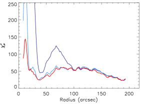
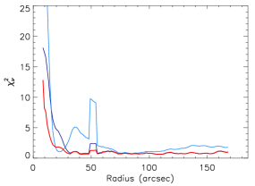
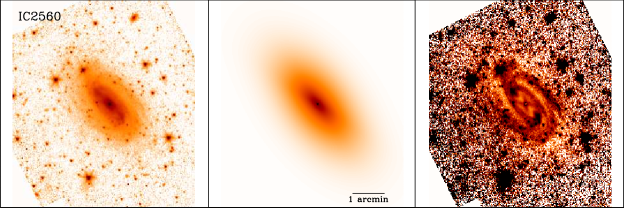
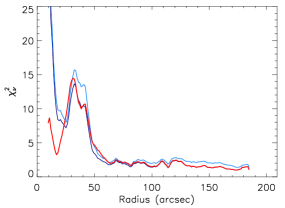
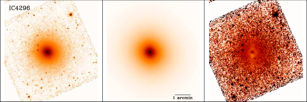
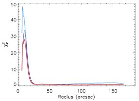
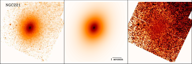
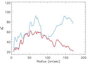
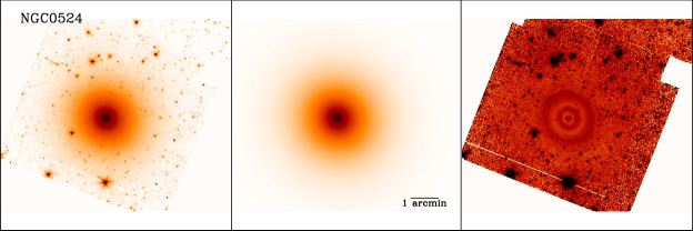
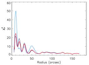
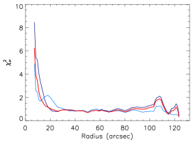
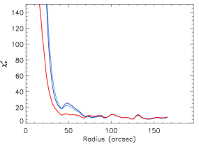
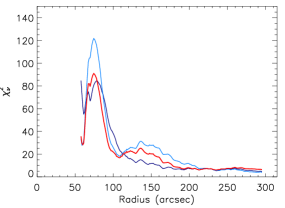
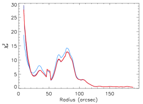
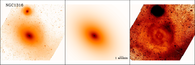
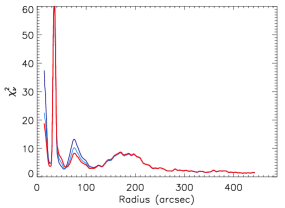
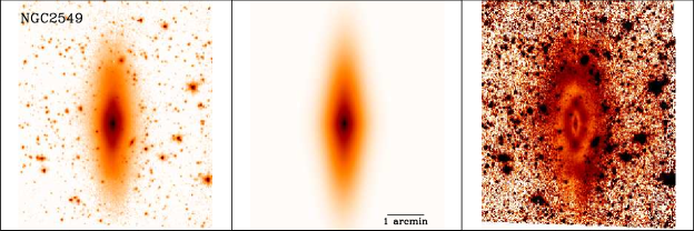
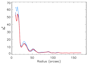
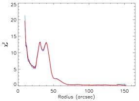
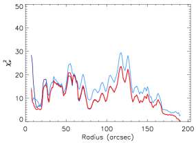
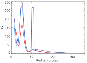
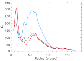
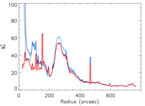
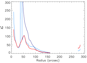
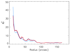
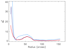
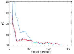
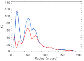
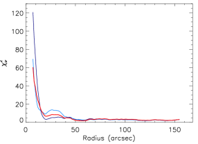
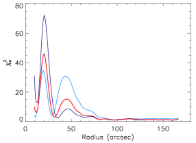
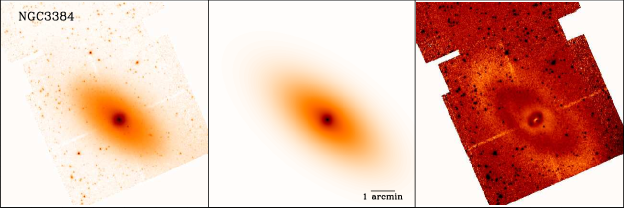
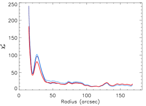
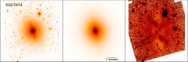
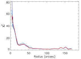
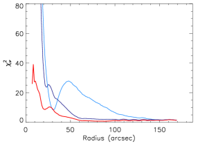
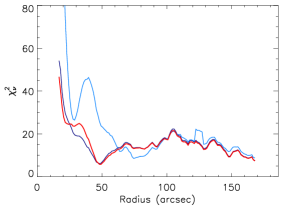
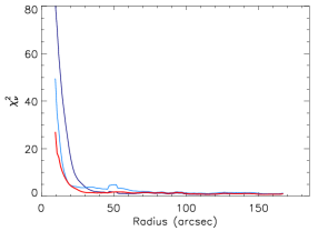
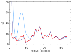
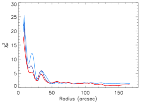
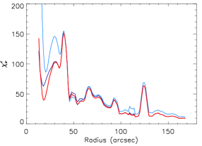
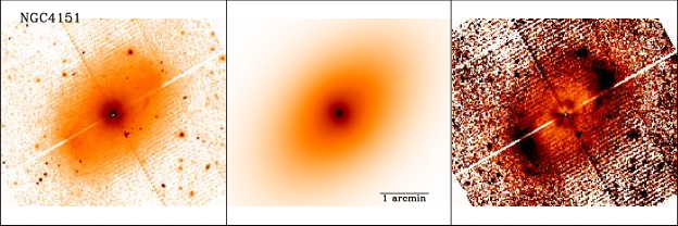
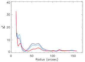
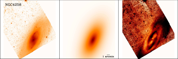
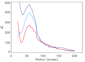
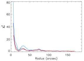
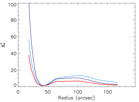
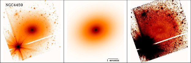
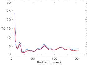
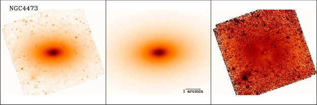
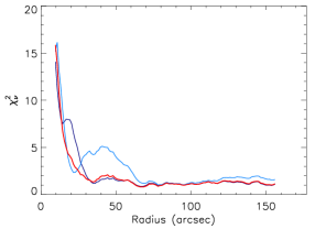
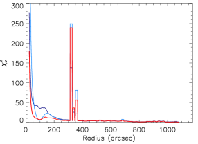
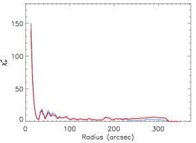
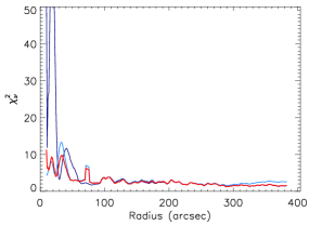
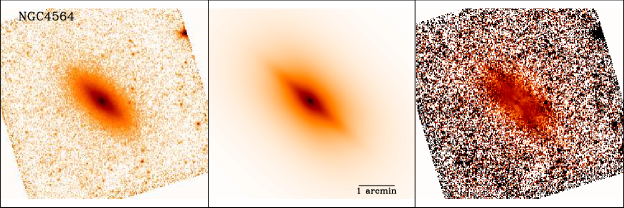
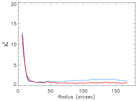
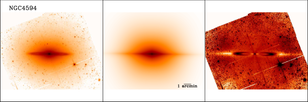
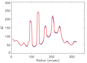
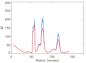
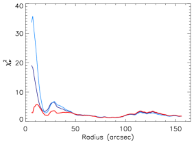
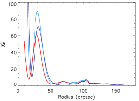
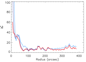
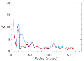
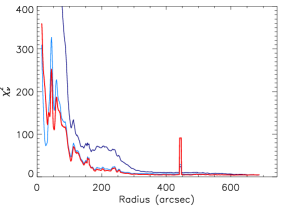
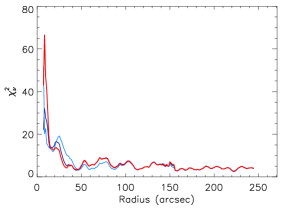
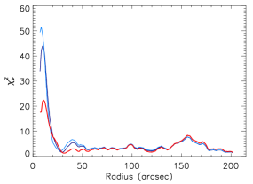
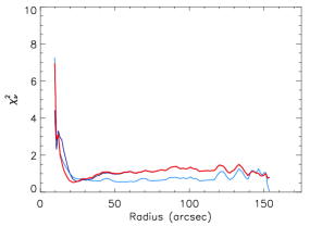
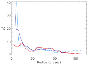
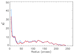
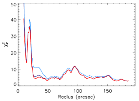
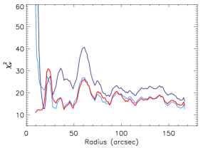
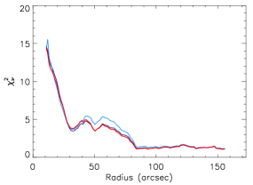
As shown by HPG04, the bulge component influences the $\chi^{2}$ value only in the inner region of the galaxy; indeed, the reduced $\chi^{2}$ depends on $n$ only at small distances (radii) from the center, while the large area of the disk strongly dilutes the influence of the bulge on the global $\chi^{2}$. Appendix A (available online) shows examples of the trend reduced $\chi^{2}$ with radii for our galaxies outlining that fits with acceptable $\chi^{2}$ values can differ significantly in the inner region where the bulge is important. Therefore, following HPG04, we selected the fits with the best $n$ and sky values considering the lowest reduced $\chi^{2}$ within half optical radius $R_{opt,0.5}$. The fits are then considered reliable on the basis of circumnuclear flux conservation; the ratio between the inner counts in the residual and source images must lower than 0.05. This means that less than $5\%$ of the central flux can be lost or introduced by the model. As described in the following section, the recovery of a tight FP at 3.6 $\mu$m  shows the accuracy of our analysis in estimating bulge structural parameters.

The absolute errors on the free parameters are derived as the variations between the best fit values and the ones obtained from the model having the closest $s,~{}s+\sigma_{s}$ or $s-\sigma_{s}$ value and the lowest possible reduced $\chi^{2}$ within $R_{opt,0.5}$ according to the criterion described above. With this choice we overestimate the statistical fit errors, but carefully constrain the effects due to an uncertain estimate of the background. The fit parameters and their uncertainties are listed in Table 3. See also Appendix A (available online) for further details on the error estimates.

2.4 The fundamental plane at 3.6 $\mu$m and the identification of pseudobulges

Early type galaxies and the bulges of disk galaxies follow the well known relations connecting their effective radius $R_{\mathrm{e}}$, mean surface brightness $<I_{e}>$ within $R_{\mathrm{e}}$, and velocity dispersion $\sigma$ (e.g. Djorgovsky & Davis 1987, Prugniel & Simien 1996, Jorgensen, Franx & Kjaergaard 1996, Burstein et al. 1997, Cappellari et al.2006). In particular, Jun & Im (2008, hereafter JI08) studied the FP at 3.6 $\mu$m considering a sample of elliptical galaxies spanning an order of magnitude in effective radii. Here, to analyze the bulge properties and verify the reliability of our analysis, we adopt the relation found by JI08:

$$\log R_{e}=1.55\times\log\sigma-0.89\times\log<I_{e}>-9.89,$$ (1)

where $\sigma$ in km/s, $R_{\mathrm{e}}$ is in kpc and $<I_{e}>$ in mag arcsec^-2.

Figure 1: MIR fundamental plane for our decomposed bulges. The 3.6 $\mu$m FP coordinate axes are given by equation (1) (JI08), represented by the black dashed line. The bulge parameters are the effective radius $R_{\mathrm{e}}$ in kpc (Tab. 3), the velocity dispersion $\sigma$ in km/s (Tab. 2) and the mean surface brightness within $R_{\mathrm{e}}$, $<\mu_{e}>=m_{bulge}+2.5\log[2\pi(b/a)_{b}R_{e}^{2}]$, where $(b/a)_{b}$ is the bulge axis ratio. $<\mu_{e}>$ is expressed in mag/arcsec² (for a consistent comparison with JI08, Vega magnitudes in Tab.3 are converted to the AB photometric system as $m$(AB)=$m$(Vega)+2.79). The color codes reflect the adopted fitting model, i.e. black points correspond to pure Sérsic profiles, blue symbols refer to Sérsic and an exponential disk (open circles), possibly with an additional Gaussian component (asterisks). The empty green triangles correspond to active galaxies, whose AGN emission is reproduced adding a point-like source to the models listed above. Open red squares highlight bulges with $n\leq 2$ which we thus classify as pseudobulges according to the FD10 criterion; no additional components are added to model these galaxies. The gray-shaded region highlights the range of velocity dispersion and surface brightness of the JI08 sample.

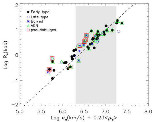
Figure 1 shows the 3.6 $\mu$m FP for all our decomposed bulges obtained by using equation (1) (dashed black line). From Fig. 1 we can draw two main conclusions: (i) our bulges follow the 3.6 $\mu$m FP of elliptical galaxies with low dispersion, and (ii) pseudobulges (open red squares) lie on the FP within the observed dispersion. Indeed, (i) if we follow JI08 and apply a maximum likelihood method with a bootstrap resampling to account for errors, the intrinsic dispersion is: $0.20\pm 0.04$ dex for the entire sample, and $0.11\pm 0.04$ dex for non-active galaxies. The last result is consistent within the errors with JI08 ($rms=0.09\pm 0.04$, private communication). Thus the presence of an AGN can slightly worsen the 2D decomposition, introducing some degeneracy with the bulge component. Nevertheless, the low dispersion of the 3.6 $\mu$m FP for our bulges and the absence of strong outliers suggests that our 2D decomposition is reliable. A tight FP and its extension to reliably compact bulges then permit us to calibrate M/L (Fig. 4 and see Section 3.2).

A detailed analysis of the FP is beyond the scope of this paper. However, it should be noted that our sample spans an order of magnitude larger range in galaxy sizes, extending the FP to smaller galaxy radii than in JI08. This could be the origin of the possible small disagreement between the FP defined by our sources and the determination by JI08 (see Fig. 1).

Classical bulges and pseudobulges differ in morphology and dynamics: the first behave like early-type galaxies, scaled to small sizes, surrounded by a disk component. Classical bulges thus are either prolate or oblate spheroids and are kinematically hot, (tending to be pressure dominated with a stellar $V/\sigma<1$). On the contrary pseudobulges are disk-like components with $V/\sigma>1$ cold kinematics dominated by rotation and possibly containing disk features such as nuclear bars and rings as well as young stellar populations (Andredakis, Peletier & Balcells 1995, Fisher & Drory 2010, hereafter FD10, and references therein). A correlation between the bulge morphology and the Sérsic index has been proposed by considering the morphological properties of pseudobulges as shown in FD10. We thus follow the FD10 Sérsic index criterion to classify those bulges in spirals and lenticulars with $n<2$ as pseudobulges. By means of the Sérsic index, we identify nine disk galaxies as hosting pseudobulges: Circinus, IC2560, NGC1068, NGC3079, NGC3368, NGC3489, NGC3998, NGC4258, NGC4594. The pseudobulges (ii) which we have identified are marked with open red squares in Fig. 1 and are not outliers of the 3.6 $\mu$m FP. This is not surprising since the physical meaning of the fundamental plane is that galaxies are virialized systems (Burstein et al. 1997) and this applies also to rotationally supported pseudobulges. Our sample partly overlaps the FD10 one, and for the 8 sources in common the classical versus pseudo classification of bulges is in perfect agreement.

3 Results

In the previous section we have verified the validity of our 2D decomposition by exploring the 3.6 $\mu$m FP for ellipticals, which turns out to be as tight as that observed by JI08 (private communication). Here we study the relations between $M_{\mathrm{BH}}$ and the bulge structural parameters listed in Tab. 2 and 3), respectively. To analyze the $M_{\mathrm{BH}}$-bulge scaling relations, we adopt three different fitting methods:

1. a bisector linear regression (Akritas & Bershady 1996), which uses the bivariate correlated errors and intrinsic scatter (BCES) method. Whereas this method takes into account the intrinsic scatter, it does not allow any determination of it. Hence the intrinsic $rms$ has been estimated with a maximum likelihood method assuming normally distributed values.

2. the linear regression FITEXY method as modified by T02, that accounts for the intrinsic scatter by adding, in quadrature, a constant value to the error of the dependent variable in order to obtain a reduced $\chi^{2}$ of 1.

3. a Bayesian approach to linear regression, LINMIX_ERR (Kelly 2007), which accounts for measurement errors, non-detections and intrinsic scatter to compute the posterior probability distribution of parameters.

The $M_{\mathrm{BH}}$-bulge relations we fit are in the following form:

$$\log M_{\bullet}/M_{\odot}=\alpha+\beta\times(x-x_{0}),$$ (2)

where $x$ is the logarithm of a measured bulge structural parameter expressed in solar units and $x_{0}$ is its mean value, used to reduce the covariance between the fit parameters. As described below, the three methods provide consistent results for the $M_{\mathrm{BH}}$-bulge relations.

Since the LINMIX_ERR is argued to be among the most robust regression methods for reliable estimates of the intrinsic dispersion (Kelly 2007), we use it to obtain the final results on the $M_{\mathrm{BH}}$-bulge scaling relations. We still use the BCES and FITEXY methods for comparison with previous works.

The fitting results are plotted in Fig. 2, 3, and 5, where we present the $M_{\mathrm{BH}}$-$L_{\mathrm{bul}}$, $M_{\mathrm{BH}}$-$M_{\mathrm{dyn}}$ and $M_{\mathrm{BH}}$-$\sigma$ relations respectively. The $M_{\mathrm{BH}}$-$\sigma$ relation is analyzed only to provide a consistent comparison with $M_{\mathrm{BH}}$-$L_{\mathrm{bul}}$ and $M_{\mathrm{BH}}$-$M_{\mathrm{dyn}}$ in terms of sample and fitting methods.

We exclude from the linear regressions the nine sources classified as pseudobulges. This allows us to verify, and possibly quantify, whether pseudobulges follow the same scaling relations as classical bulges. From a visual inspection of Fig. 2-5, pseudobulges with large BH masses ($M_{\mathrm{BH}}$$>10^{7}$$M_{\odot}$) follow the relations while those with low BH masses deviate significantly from the scaling relations defined by classical bulges. Deviant pseudobulges are analyzed in the following sections and discussed in Section 4.

In the following, after describing in details the $M_{\mathrm{BH}}$-bulge relations at 3.6 $\mu$m, we compare them with the published results obtained at shorter wavelengths. Finally in Section 3.4 we explore the possible $M_{\mathrm{BH}}$ correlation with $\sigma$ and $R_{e}$ separately as suggested by MH03, Hopkins et al. 2007, Graham 2008a.

3.1 $M_{\mathrm{BH}}$ versus 3.6 $\mu$m bulge luminosity

Figure 2: Scaling relations. The $M_{\mathrm{BH}}$ as a function of 3.6 $\mu$m luminosity. The linear regressions are shown as dot dashed blue, dashed green and red continuous lines respectively for the BCES, FITEXY and LINMIX_ERR methods and are obtained from classical bulges only (47 sources). Pseudobulges are open red squares.

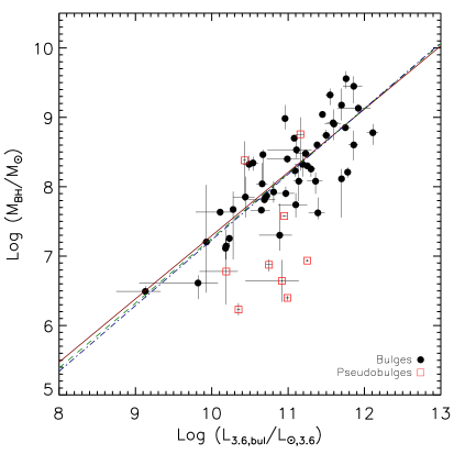
To construct the $M_{\mathrm{BH}}$-$L_{\mathrm{3.6,bul}}$ correlation, we compute the bulge 3.6 $\mu$m luminosity using the magnitudes obtained with the two-dimensional decomposition (see Section 2.3 for details) and reported in Tab. 3. To derive 3.6 $\mu$m luminosities in solar units we use the 3.6 $\mu$m Solar absolute magnitude obtained with a K-band value of 3.3 mag and a K-[3.6]=0.05 mag color correction (Allen 1976, see also Bessell & Brett 1988, Bell & De Jong 2001). The data for classical bulges are fitted with the three linear regression methods described at the beginning of this section. We obtain the following scaling relation of $M_{\mathrm{BH}}$ with 3.6 $\mu$m bulge luminosity (see Tab. 4 for the results from all fitting methods):

$$\log M_{\mathrm{BH}}/M_{\odot} = (8.19\pm 0.06)+$$

$$(0.93\pm 0.10)\times[\log(L_{\mathrm{3.6,bul}}/L_{3.6,\odot})-11]$$

$$[rms=0.38\pm 0.05]$$

LINEAR REGRESSION COEFFICIENTS

$\log(M_{\mathrm{BH}})-\log(x)$ $x_{0}$ Method $\alpha$ $\beta$ $rms$ Ref. 11.0 BCES $8.18\pm 0.06$ $0.95\pm 0.10$ $0.35\pm 0.02$ - $M_{\mathrm{BH}}$-$L_{\mathrm{3.6,bul}}$ 11.0 FITEXY $8.21\pm 0.06$ $0.91\pm 0.10$ $0.35\pm 0.05$ - 11.0 LINMIX_ERR $8.19\pm 0.06$ $0.93\pm 0.10$ $0.38\pm 0.05$ - 10.9 BCES $8.21\pm 0.07$ $1.13\pm 0.12$ $0.31$ MH03^a $L_{bul,K}$ 10.9 FITEXY $8.29\pm 0.08$ $0.93\pm 0.10$ $0.33$ G07 10.9 BCES $8.38\pm 0.05$ $0.97\pm 0.08$ $0.36$ H09 $L_{bul,V}$ 11.0 MAX. LIKE.$\dagger$ $8.95\pm 0.11$ $1.11\pm 0.18$ $0.38$ G09^b 10.3 BCES $8.41\pm 0.11$ $1.40\pm 0.17$ - L07$\ddagger$ 11.0 BCES $8.18\pm 0.06$ $0.83\pm 0.08$ $0.33\pm 0.02$ - 11.0 FITEXY $8.20\pm 0.06$ $0.80\pm 0.08$ $0.35\pm 0.05$ - $M_{\mathrm{BH}}$-$M_{\mathrm{dyn}}$ 11.0 LINMIX_ERR $8.20\pm 0.06$ $0.79\pm 0.09$ $0.37\pm 0.05$ - 10.9 BCES $8.28\pm 0.06$ $0.96\pm 0.07$ $0.25$ MH03^a 11.0 BCES $8.20\pm 0.10$ $1.12\pm 0.06$ $0.30$ HR04 10.9 BCES $8.61\pm 0.05$ $0.88\pm 0.06$ $0.27$ H09 11.0 BCES $8.15\pm 0.05$ $0.80\pm 0.08$ $0.35\pm 0.03$ - $M_{\mathrm{BH}}$-$M_{\star}$ 11.0 FITEXY $8.17\pm 0.06$ $0.77\pm 0.08$ $0.35\pm 0.05$ - 11.0 LINMIX_ERR $8.16\pm 0.06$ $0.79\pm 0.08$ $0.38\pm 0.05$ - 11.0 BCES $8.24\pm 0.05$ $1.07\pm 0.09$ $0.32$ H09 200 BCES $8.27\pm 0.05$ $4.0\pm 0.3$ $0.32\pm 0.04$ - $M_{\mathrm{BH}}$-$\sigma$ 200 FITEXY $8.30\pm 0.05$ $4.0\pm 0.3$ $0.30\pm 0.04$ - 200 LINMIX_ERR $8.29\pm 0.05$ $4.0\pm 0.4$ $0.33\pm 0.04$ - $M_{\mathrm{BH}}$-$\sigma$ 200 FITEXY $8.13\pm 0.06$ $4.0\pm 0.3$ $0.3$ T02 $M_{\mathrm{BH}}$-$\sigma$ 200 MAX. LIKE. $8.23\pm 0.08$ $4.0\pm 0.4$ $0.31\pm 0.06$ G09^b

Table 4: Linear regression coefficients of $M_{\mathrm{BH}}$ as a function of the bulge property $x$, starting from the top of column (1): bulge 3.6 $\mu$m luminosity (equation LABEL:eq:l) compared with previous works and with K and V band results; bulge dynamical (equation 5) and stellar (equation LABEL:eq:mst) masses; bulge velocity dispersion (equation LABEL:eq:s) and effective radius (equation LABEL:eq:re). The coefficients are obtained using the normalizations in column (2) and with the methods listed in column (3). $\dagger$ G09 use a generalized maximum likelihood method to account for upper limits. Columns (4)-(6) list the intercept, slope and rms (in dex) respectively. We compare our results with the works listed in column (7). $\ddagger$ Lauer et al. (2007). ^a Coefficients obtained cutting the sample on the basis of the sphere of influence argument for the $M_{\mathrm{BH}}$ estimates. ^b Coefficients obtained only for elliptical galaxies.

All the fit parameters obtained with the three different methods are consistent within the errors (see Tab. 4, and Fig. 2). Our results are in excellent agreement with the $M_{\mathrm{BH}}$-L_bul,λ obtained at shorter wavelengths. More specifically using the BCES and FITEXY results for the comparison, the intercept, slope and $rms$ are fully consistent with the K-band measurements of MH03, Graham (2007), and H09. We find an intrinsic dispersion for the $M_{\mathrm{BH}}$-$L_{\mathrm{3.6,bul}}$ scaling relation with $rms=0.35\pm 0.05$dex (BCES, FITEXY in Tab.4), consistent with the correlation in the K-band: $rms=0.31$ and $0.36$ dex in MH03 and H09 respectively. Optical observations in the V-band (Lauer et al. 2007, G09) produce slightly higher values for $\alpha$ and $\beta$. Different linear correlation coefficients can be due to a combination of factors: most obviously color corrections, but also incomplete sample overlap and the range of Hubble types (G09 fit only early types). Furthermore our $M_{\mathrm{BH}}$-$L_{\mathrm{3.6,bul}}$ is tighter than the V-band correlation whose $rms$ is $0.38\pm 0.09$ for early-type galaxies only. Moreover extinction can affect the luminosity, especially the V-band.

Figure 2 illustrates that 4 out of 9 pseudobulges (NGC3489, NGC3998, NGC4258, NGC4594) are consistent with the correlation for classical bulges, while the others (CIRCINUS, IC2560, NGC1068, NGC3079, NGC3368) are outliers, at more than $4\sigma$ below the LINMIX_ERR linear regression. The poor statistics for pseudobulges prevent us from drawing firm conclusion on the physical nature of this behavior. Nevertheless we examine the possible disagreement also for the other $M_{\mathrm{BH}}$ linear regressions in Section 4.

3.2 $M_{\mathrm{BH}}$ versus bulge mass

In this section we first describe two methods to derive the bulge mass, and then relate $M_{\mathrm{BH}}$ with $M_{\mathrm{dyn}}$ and $M_{\star}$. Indeed one of our aims is to verify whether the 3.6 $\mu$m waveband is suitable to investigate the $M_{\mathrm{BH}}$-bulge mass relations. We determine (i) the bulge dynamical mass $M_{\mathrm{dyn}}$ by applying the virial theorem (as in MH03, H09), and (ii) the bulge stellar mass by calibrating the M/L as a function of the 3.6 $\mu$m luminosity both with and without V-[3.6] and K-[3.6] colors. Thus (i) the bulge $M_{\mathrm{dyn}}$ is computed as follows:

$$M_{dyn}=\kappa R_{e}\sigma^{2}/G,$$ (4)

where G is the gravitational constant, $\sigma$ and R_e the velocity dispersion (in Tab.2) and the bulge effective radius (in Tab. 3) respectively. It is generally assumed that bulges behave as isothermal spheres and the factor $\kappa$ is usually fixed at a value of 3 (Gebhardt et al. 2003) or 8/3 (MH03). However, since bulges are well reproduced by Sérsic profiles, $\kappa$ is in general a function of the Sérsic index $n$. Cappellari et al. (2006), using full dynamical models, provide the $\kappa(n)$ relation for classical bulges and show that even the use of a constant average value of $\bar{\kappa}=5$ can provide an accurate estimate of $M_{\mathrm{dyn}}$ to within 0.10 dex.  We have therefore adopted $\bar{\kappa}=5$.

The $M_{\mathrm{BH}}$-$M_{\mathrm{dyn}}$ bulge relation shown in Fig. 3A together with the three linear regressions. The $M_{\mathrm{dyn}}$ dependence for the 47 classical bulges is:

$$\log M_{\mathrm{BH}}/M_{\odot} = (8.20\pm 0.06)+$$

$$(0.79\pm 0.09)\times[\log(M_{\mathrm{dyn}}/M_{\odot})-11]$$

$$[rms=0.37\pm 0.06]$$

(5)

Figure 3: Scaling relations. The $M_{\mathrm{BH}}$ as a function of bulge dynamical mass (panel a) and bulge stellar mass (panel b). Pseudobulges are highlighted as red open squares. In panel (b) the M/L is from equation LABEL:eq:mll. See Section 3.2 and Fig. 4 for details on the M/L calibrations.

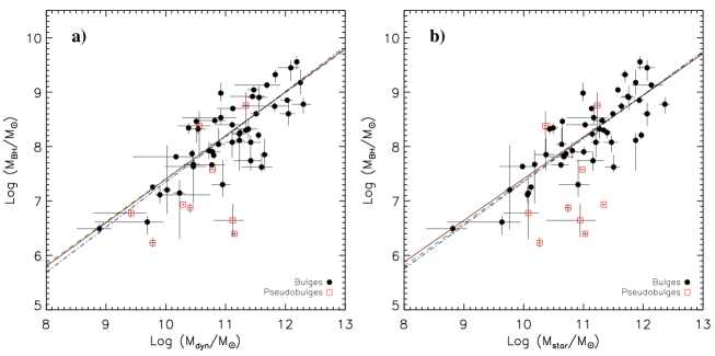
The three linear regressions are consistent within the errors (See Tab. 4, Fig. 3A). The $M_{\mathrm{BH}}$-$M_{\mathrm{dyn}}$ relation is rather tight with an $rms\sim 0.35$ dex from LINMIX_ERR, comparable to the scatter in the $M_{\mathrm{BH}}$-$\sigma$ function (see Section 3.3). The $M_{\mathrm{BH}}$-$M_{\mathrm{dyn}}$ relations are in excellent agreement with the similar K-band analysis in MH03 and H09. The BCES regression is also consistent with a sample of 30 galaxies by HR04 although their slope is slightly superlinear.

The position of pseudobulges is the same observed in Fig. 2 and described in Section 3.1, where about half of the pseudobulges lie more than $4\sigma$ below the regression. The result for dynamical bulge mass can be compared with those for stellar mass to assess wether there are discrepancies between the two relations with $M_{\mathrm{BH}}$.

To estimate (ii) the bulge stellar mass $M_{\star}$ we have calibrated the M/L ratio at 3.6 $\mu$m through color corrections. It is known that the M/L ratio is wavelength dependent and not constant for a spiral galaxy in any waveband. M/L trends have been found to be minimized in the K-band (Bell & de Jong 2001, Bell et al. 2003). Published works assume a constant M/L with radius, while we are interested in the M/L for the bulge alone. The 3.6 $\mu$m wavelength is in principle a good tracer of stellar light for both young and old stellar populations as well, thus our data are expected to trace M/L with a low scatter. Moreover the extent of our FP to compact sizes, its tight dispersion valid for all Hubble types, and the agreement with the 3.6 $\mu$m FP observed for pure elliptical galaxies should guarantee a reliable estimate for the M/L of our bulges.

Figure 4: $M_{\mathrm{dyn}}$ versus $L_{\mathrm{3.6,bul}}$. The black line represents the linear regression of equation (LABEL:eq:mll).

We assume that $M_{\mathrm{dyn}}$ in bulges is dominated by the stellar mass, with a negligible contribution of dark matter and gas (Drory, Bender & Hopp 2004; Padmanabhan et al. 2004). We then consider our sample of spheroids (49 sources, see Tab.2) and fit a linear relation to $M_{\mathrm{dyn}}$, computed as in equation (4), vs $L_{\mathrm{3.6,bul}}$ as:

$$\log M_{\mathrm{dyn}} = (11.04\pm 0.03)+$$

$$(1.18\pm 0.07)\times[\log(L_{\mathrm{3.6,bul}}/L_{3.6,\odot})-11]$$

$$[rms=0.13\pm 0.04]$$

This is determined using LINMIX_ERR and is very tight with $rms\sim 0.10$. A tight $M_{\mathrm{dyn}}$-$L_{\mathrm{3.6,bul}}$ relation is not unexpected as it is just a different way (i.e. $\sigma^{2}$$R_{\mathrm{e}}$ vs $L_{\mathrm{3.6,bul}}$) to express the FP. The $M_{\mathrm{dyn}}$-$L_{\mathrm{3.6,bul}}$  relation is shown in Fig. 4.

We now include a color correction to test how it affects the M/L ratio. Only 25 sources are included in this exercise, i.e. those whose classical bulges having V- and K- magnitudes available in the literature (listed in Tab. 2). This allows a comparison with the above calibration and the following multi-linear regression:

$$\log M_{\mathrm{dyn}} = (11.00\pm 0.05)+$$

$$(1.35\pm 0.11)\times[\log(L_{\mathrm{3.6,bul}}/L_{3.6,\odot})-11]$$

$$+(0.07\pm 0.10)\times[(V-K)-2.54]$$

$$[rms=0.11\pm 0.06]$$

where we add V-K color correction relative to the sample mean V-K color. The fit was performed using the multivariate extension of LINMIX_ERR (MLINMIX_ERR, Kelly 2007). The zeropoints and slopes of $L_{\mathrm{3.6,bul}}$  in equation (LABEL:eq:mll) and (LABEL:eq:multi) are the same, as well as intrinsic dispersions, while the slope of $(V-K)$ is consistent with zero within the errors. This, clearly indicates that M/L for bulges is not affected by the V-K color and the 3.6 $\mu$m waveband is confirmed to be a better tracer of the stellar light than the K-band for both old and young stellar populations. With the $M_{\mathrm{dyn}}$-$L_{\mathrm{3.6,bul}}$ relation we have (i) calibrated the M/L ratio for the bulge component independently of the Hubble type of our galaxies, (ii) demonstrated how the 3.6 $\mu$m passband traces the stellar bulge mass better than optical or near-infrared colors for both young and old stellar populations, and finally (iii) found that V- and K- colors do not strongly influence $M_{\star}$ determinations based on $L_{\mathrm{3.6,bul}}$.

Figure 3B shows the $M_{\mathrm{BH}}$-$M_{\star}$ linear regressions:

$$\log M_{\mathrm{BH}}/M_{\odot} = (8.16\pm 0.06)+$$

$$(0.79\pm 0.08)\times[\log(M_{\star}/M_{\odot})-11]$$

$$[rms=0.38\pm 0.05]$$

where we use equation (LABEL:eq:mll) to calibrate $M_{\star}$. Equation (LABEL:eq:mst) is just the $M_{\mathrm{BH}}$-$L_{\mathrm{3.6,bul}}$ relation rescaled using equation (LABEL:eq:mll) to determine $M_{\star}$, in order to obtain a relation where $M_{\star}$ is derived by the host luminosity as done in studies at high redshifts (e.g. Merloni et al. 2010). Thus the black hole vs bulge mass correlation can be used as the reference scaling relation in the local Universe to probe a possible evolution of $M_{\mathrm{BH}}$-$M_{\star}$. This issue is discussed in Section 4. The coefficients and rms of equation (LABEL:eq:mst) are consistent within the errors with the $M_{\mathrm{BH}}$-$M_{\mathrm{dyn}}$ scaling relation (for our choice fitting method, see equation (5), and Tab. 4). H09 find a steeper slope, but the use of an extinction corrected B-V color to calibrate M/L in the K band possibly affect the resulting $M_{\mathrm{BH}}$-$M_{\star}$. The M/L calibration presented here provide a robust estimate for $M_{\star}$; this issue is pursued further in Section 4.

3.3 A comparison with the $M_{\mathrm{BH}}$-$\sigma$ relation

In the previous sections we have analyzed all the $M_{\mathrm{BH}}$-bulge scaling relations which can be obtained using results from our bi-dimensional decomposition. We found (i) the same intrinsic dispersion for all the scaling relations $rms\sim 0.35$ dex, and (ii) that pseudobulges have a bimodal distribution with half of them lying on the relations within the observed scatter, while those harboring smaller BHs ($M_{\mathrm{BH}}$$\leq 10^{7}$$M_{\odot}$) significantly deviate from the regression. Here we compare our $M_{\mathrm{BH}}$- bulge relations with $M_{\mathrm{BH}}$-$\sigma$. A detailed analysis of the $M_{\mathrm{BH}}$-$\sigma$ relation is beyond the scope of this paper, our aim is just to obtain a consistent comparison of $M_{\mathrm{BH}}$-$\sigma$ with the other relations in terms of samples and fitting method.

Figure 5: Scaling relations. The $M_{\mathrm{BH}}$ is plotted as a function of velocity dispersion. The linear regressions and symbols are as in Fig. 2.

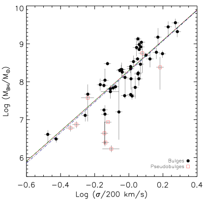
The classical bulges lie on the following correlation:

$$\log M_{\mathrm{BH}} = (8.29\pm 0.05)+$$

$$(4.0\pm 0.4)\times\log(\sigma/200~{}km\,s^{-1})$$

$$[rms=0.33\pm 0.04]$$

In equation (LABEL:eq:s) the velocity dispersion is normalized at 200 km/s according to T02, G09. Figure 5 displays $M_{\mathrm{BH}}$ as a function of $\sigma$ and the three linear regressions, with the parameters in Tab. 4.

Although the samples do not fully overlap, our BCES and FITEXY results are in good agreement with G09 and T02. More interesting is the correspondence, within the errors, between the $M_{\mathrm{BH}}$-$M_{\mathrm{dyn}}$ ($M_{\star}$, $L_{\mathrm{3.6,bul}}$) and $M_{\mathrm{BH}}$-$\sigma$ intrinsic scatters ($rms\sim 0.3-0.35$ dex). Thus at 3.6 $\mu$m is not possible to assess whether the bulge dynamics or luminosity drive the observed scaling relations.

As expected, some, but not all, the pseudobulges are displaced from the inferred regressions. These are CIRCINUS, IC2560, NGC1068, NGC3079 and NGC3998; therefore there is a good overlap (4/6 where the exceptions are NGC3368 and NGC3998) with the deviant pseudobulges found in the previous sections. This discrepancy, also found in H09 and Nowak et al. 2010, could arise from several different causes; there could be an additional nuclear component not identified with our image 2D decomposition; or e. g. pseudobulges could have a different evolutionary history than classical bulges. We defer a detailed discussion to the following section.

Figure 6: Scaling relations. The $M_{\mathrm{BH}}$ is plotted as a function of the bulge effective radius $R_{\mathrm{e}}$. The linear regressions and symbols are as in Fig. 2.

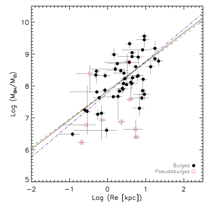
3.4 $M_{\mathrm{BH}}$ versus $R_{\mathrm{e}}$, the effective radius at 3.6 $\mu$m

Figure 7: $M_{\mathrm{BH}}$ (in Tab.2) residuals about their $M_{\mathrm{BH}}$-$\sigma$ relation (Eq LABEL:eq:s) versus $R_{\mathrm{e}}$. The dashed line represents null residuals. Black points are early- and late- type galaxies, blue asterisks are barred galaxies and open red squares are pseudobulges.

$M_{\mathrm{BH}}$ has been observed to be separately related to the bulge stellar velocity dispersion $\sigma$ and its effective radius $R_{\mathrm{e}}$. This has been first observed in MH03 by a partial correlation analysis. Figure 6 shows the $M_{\mathrm{BH}}$-$R_{\mathrm{e}}$ relation obtained with our 3.6 $\mu$m 2D decomposition, where the LINMIX ERR method gives:

$$\log M_{\mathrm{BH}} = (8.22\pm 0.08)+$$

$$(0.88\pm 0.17)\times[\log(R_{\mathrm{e}}/kpc)-0.4]$$

$$[rms=0.54\pm 0.07]$$

The three linear regression in Tab. 4 are in good agreement within the errors. The intrinsic dispersion is significantly larger than in other relations. Nevertheless the possible existence of $M_{\mathrm{BH}}$-$R_{\mathrm{e}}$ is intriguing and prompts investigation of a possible fundamental plane for BHs, in analogy with the galaxies FP.

It is still unclear whether one $M_{\mathrm{BH}}$-bulge relation is significantly tighter than the others. Hopkins et al. (2007) explained the lack of a dominant $M_{\mathrm{BH}}$-bulge scaling relation because each of them is the projection of the same fundamental plane relating $M_{\mathrm{BH}}$ with two or more bulge properties. However, the issue of a BH fundamental plane is still matter of debate: Graham 2008a showed that the need for a $M_{\mathrm{BH}}$ fundamental plane originates on a displacement of barred galaxies with respect to the residuals of the $M_{\mathrm{BH}}$-$\sigma$ relation.

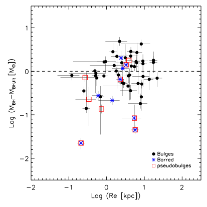
If a $M_{\mathrm{BH}}$ FP actually exists, it should be easily observed at 3.6 $\mu$m. Thus here we follow MH03 and Graham (2008a) and compare the residuals of $M_{\mathrm{BH}}$-$\sigma$ for our bulges (expressed in equation LABEL:eq:s) with the effective radius (column 4 in Tab. 3). Figure 7 shows this comparison where we highlight the position of barred galaxies and pseudobulges. Hence, we check for a possible significant correlation performing both the Pearson and Spearman rank correlation test. As shown in Tab.5, there is no significant correlation either for the entire sample or excluding barred galaxies and/or pseudobulges.

STATISTICAL TESTS FOR $M_{\mathrm{BH}}$ RESIDUALS

Sample Test $\rho$ significance all galaxies Spearman 0.22 0.10 Pearson 0.29 - no barred Spearman 0.21 0.16 Pearson 0.29 - no pseudobulges Spearman 0.16 0.26 Pearson 0.24 - no pseudobulges, Spearman 0.11 0.48 no bar Pearson 0.20 -

Table 5: Statistical test for the $M_{\mathrm{BH}}$ residuals about their $M_{\mathrm{BH}}$-$\sigma$ correlation with $R_{e}$ in Fig. 7. Column 1: tests are performed for the total sample and sub-samples excluding barred galaxies and pseudobulges. Column 2: the kind of statistic applied to data (Spearman rank correlation and Pearson correlation). Column 3: correlation coefficient $\rho$. Column 4: and the two-sided significance of $\rho$ deviation from zero in the Spearman rank correlation. The significance is a value in the interval [0.0, 1.0]; a value consistent with zero indicates a significant correlation.

Thus, our analysis at 3.6 $\mu$m does not confirm the existence of BH FP. We refer to a forthcoming paper (Marconi et al. 2011 in prep.) for a detailed study of the origin of the FP for supermassive BHs.

4 Discussion

The high signal-to-noise images provided by Spitzer/IRAC and our improved 2D analysis have allowed us to obtain accurate estimates of bulge luminosities and effective radii at 3.6 $\mu$m, as demonstrated by the tight fundamental plane and $M_{\mathrm{dyn}}$-$L_{\mathrm{bul}}$ relations. We have been able to (i) calibrate the $M_{\star}$-$L_{\mathrm{bul}}$ relation, accurate to $0.10\pm 0.05$ rms without any color correction and (ii) securely define pseudobulges through the Sérsic index value ($n\leq 2$) and study their location with respect to the scaling relations for classical bulges. We have then obtained the $M_{\mathrm{BH}}$-galaxy relations for classical bulges using our photometry at 3.6 $\mu$m. They are expressed in Eqs. LABEL:eq:l, 5, and LABEL:eq:mst, and shown in Figs. 2, 3 and 5.

All the above scaling relations have an intrinsic dispersion of 0.35 dex (from a Bayesian approach to linear regression, see Tab.4) and are in perfect agreement with the $M_{\mathrm{BH}}$-$\sigma$ relation for our galaxies in equation (LABEL:eq:s). Considering the methods adopted in literature to perform linear regressions that account for the intrinsic scatter (BCES and FITEXY) our 3.6 $\mu$m correlations are as tight as the $M_{\mathrm{BH}}$- bulge K-band luminosity (MH03, H09) and tighter than in V-band (G09). Moreover the $M_{\mathrm{BH}}$-$M_{\mathrm{dyn}}$ and $M_{\mathrm{BH}}$-$M_{\star}$ agree very well with MH03, HR04 and H09, with the new advantage of an accurate M/L relation for bulges at 3.6 $\mu$m calibrated without any color correction.

Figure 3 present the $M_{\mathrm{BH}}$-$M_{\star}$ relation, where $M_{\star}$ is obtained by combining $L_{\mathrm{bul}}$ with our calibrated $M_{\star}$-$L_{\mathrm{bul}}$ relation. This relation represents the reference $M_{\mathrm{BH}}$-$M_{\star}$ in the local Universe for studies of the $M_{\mathrm{BH}}$-galaxy scaling relations at higher z, based on $M_{\star}$ derived from luminosity measurements (Merloni et al. 2010, Trakhtenbrot & Netzer 2010). The $z$ evolution of $M_{\mathrm{BH}}$-galaxy scaling relations has been studied in several papers but remains controversial. For instance, Woo et al. (2008) report a significant evolution of the BH-bulge relations at $z=0.3-0.6$, with larger BH masses for given bulge $\sigma$/luminosity with respect to local values. This evolution is however not found by Labita et al. (2009) or Shen et al. (2008). Shields et al. (2003) find no evolution of $M_{\mathrm{BH}}$-$\sigma$ up to z$\sim 2$ but using [OIII] line width as a surrogate for $\sigma$. Indeed, at high redshift a dynamical measurement of the bulge mass based on $\sigma$ is difficult due to the limited signal-to-noise and spatial resolution. On the contrary the total stellar mass of the host galaxy is relatively easier to estimate from host galaxy luminosities and colors (e.g. Peng et al. 2006), or by deconvolving AGN and galaxy spectral energy distributions (Merloni et al. 2010) or by applying the correlation between the AGN bolometric luminosity and $M_{\mathrm{BH}}$ together with the relation between the star formation rate and $M_{\star}$ in star forming galaxies (Trakhtenbrot & Netzer 2010). The above observational works suggest that the $M_{\mathrm{BH}}$/$M_{\star}$ at high redshift is significantly higher than the local value. In any case, observations at high redshifts are fundamental to constrain models of BH-galaxy coevolution and to probe different paths followed by galaxies during their evolution and the building up of the $M_{\mathrm{BH}}$-bulge relations (Lamastra et al. 2010 and references therein).

In Section 3.2, the tight $M_{\mathrm{dyn}}$-$L_{\mathrm{3.6,bul}}$ relation with negligible color corrections justifies the validity of 2D decomposition to measure M/L at 3.6 $\mu$m. This (i) unveils the capability of our $M_{\mathrm{BH}}$-$M_{\mathrm{dyn}}$ (and thus $M_{\star}$) to be a suitable benchmark to probe the $M_{\mathrm{BH}}$-bulge co-evolution and to constrain theoretical models. In fact, in the next decade the instruments onboard the James Webb Space Telescope (JWST) will increase the possibility to further explore with unprecedented accuracy this waveband.

The other (ii) intriguing result found here is related to the behavior of pseudobulges. The displacement of pseudobulges, located below the scaling relations, is reported in H09 and Nowak et al. (2010). In §2.4 we followed FD10 and identified 9 pseudobulges with Sérsic index $n\leq 2$. Of these, CIRCINUS, IC2560, NGC1068, and NGC3398 lie below all the $M_{\mathrm{BH}}$ scaling relations; NGC3368 deviates from $M_{\mathrm{BH}}$-$L_{\mathrm{3.6,bul}}$, -$M_{\mathrm{dyn}}$but not from $M_{\mathrm{BH}}$-$\sigma$, while the contrary happens for NGC3998. The other pseudobulges NGC3489, NGC4258, NGC4374, NGC4594 are within the observed scatter. As mentioned in §3.3 this discrepancy can arise from several causes. We first note that the $n\leq 2$ is a statistical property of pseudobulges; indeed the tails of the Sérsic index distributions for classical and pseudobulges overlaps around $n\sim 2$ (see Fig. 9 in Fisher & Drory 2008 and FD10). Thus, not all bulges with a low $n$ would be actual pseudobulges from the dynamical point of view (Gadotti 2009).

Anyway, it is interesting to explore the possible explanations once we assume that all the nine galaxies actually harbor a pseudobulge.

(1) Additional nuclear component on small scales ($\simeq 10$ arcsec), such as bars, ovals and lenses are observed not only in disks but also in S0 galaxies (Laurikainen et al. 2009). With the grid method applied for 2D fitting (see §2.3), an additional component on small image scales of 10-15 pixels can not be taken into account, because (a) it is difficult to constrain input parameters while automatically running the fits, and (b) the model does not require any additional component to match our quality criteria (see §2.3).

(2) Nowak et al. (2010) define NGC3368 and NGC3489 as pseudobulges by resolving the nuclear dynamics, and find the coexistence of a classical bulge with a pseudobulge, where the $M_{\mathrm{BH}}$ seems to better correlate with the classical bulge alone. For the same reasons outlined above, it is beyond the possibilities of our analysis to deconvolve the classical bulge from the pseudobulge component.

(3) The nine pseudobulges could be in different evolutionary stages. Montecarlo simulations in Lamastra et al. (2010) show how in the buildup of the local $M_{\mathrm{BH}}$-$M_{\star}$ relation, galaxies can follow various evolutionary paths that proceed from below the correlation and reach their final position passing above it. Thus, the position of each source could just be the result of the different evolutionary paths being followed.

(4) Finally, nuclear star clusters (NSCs) may be common in those spheroid with $M_{\star}$$\sim 10^{8}-10^{11}$ $M_{\odot}$ harboring a $M_{\mathrm{BH}}$$<10^{7}$ $M_{\odot}$, and may contribute significantly at the mass of the central object increasing its value of a factor of $\sim 2$ (Graham & Spitler 2009 and references therein). A larger value of $M_{\mathrm{BH}}$ can prevent the coexistence of a NSC, because the very central stars should be either disrupted by the BH gravity or kicked away by tidal forces. Moreover Graham & Spitler (2009) derive a linear regression between the nuclear mass (BH plus NSC) and the stellar mass of the host spheroid. Thus, the proper quantity to be plotted on the y-axis seems to be $M_{\mathrm{BH}}$ plus the NSC mass, at least for $M_{\mathrm{BH}}$$<10^{7}$ $M_{\odot}$. The identification of NSCs requires the highest spatial resolutions available with the current instrumentation and can not be reached with Spitzer even for the closest of our sources.

We conclude that the observed displacement of pseudobulges could arise from observational limitations, true evolution, or a combination of the two.

5 Conclusions

In this work we have investigated the scaling relations observed in the local Universe between $M_{\mathrm{BH}}$ and the structural parameters of the host bulges. The analysis is based on a 2D decomposition of 3.6 $\mu$m Spitzer/IRAC images of 57 early- and late- type galaxies with $M_{\mathrm{BH}}$ measurements. Given the well known degeneracy between the bulge Sérsic index $n$ and effective radius $R_{\mathrm{e}}$, we have adopted a grid-method to fit IRAC images and determine $n$ rather than let it freely vary. The accuracy of our analysis is verified by the agreement of our bulges with the mid-infrared fundamental plane determination by JI08. Our galaxies extend their 3.6 $\mu$m FP by doubling the $R_{\mathrm{e}}$ range towards smaller radii and none of our galaxies deviate significantly from the JI08 FP. This allows us to reliably (i) calibrate M/L at 3.6 $\mu$m, (ii) study the $M_{\mathrm{BH}}$- scaling relation and (iii) identify pseudobulges in our sample.

We obtained a tight ($rms=0.10$ dex) $M_{\mathrm{dyn}}$-$L_{\mathrm{3.6,bul}}$ relation:

$$\log M_{\mathrm{dyn}}/M_{\odot}=11.04+1.18\times[\log(L_{\mathrm{3.6,bul}}/L_{3.6,\odot})-11],$$

which allows us to estimate stellar masses based on luminosities at 3.6 $\mu$m with high accuracy. The 3.6 $\mu$m luminosity appears to be the best tracer of $M_{\star}$ yet found.

The relations between $M_{\mathrm{BH}}$, luminosity, masses, and effective radius, fitted with a Bayesian approach to linear regression are:

$$\log M_{\mathrm{BH}}/M_{\odot}=8.19+0.93\times[\log(L_{\mathrm{3.6,bul}}/L_{3.6,\odot})-11],$$

$$\log M_{\mathrm{BH}}/M_{\odot}=8.20+0.79\times[\log(M_{\mathrm{dyn}}/M_{\odot})-11],$$

$$\log M_{\mathrm{BH}}/M_{\odot}=8.16+0.79\times[\log(M_{\star}/M_{\odot})-11],$$

$$\log M_{\mathrm{BH}}/M_{\odot}=8.22+0.9\times[\log(R_{\mathrm{e}}/kpc)-0.4],$$

all with the same intrinsic dispersion of $rms\sim 0.35$ dex except for $M_{\mathrm{BH}}$-$R_{\mathrm{e}}$ which has $rms\sim 0.5$ dex. Our $M_{\mathrm{BH}}$-$M_{\star}$ relation can be used as the local reference for high redshift studies which probe the cosmic evolution of $M_{\mathrm{BH}}$-galaxy scaling scaling relations.

These 3.6 $\mu$m $M_{\mathrm{BH}}$-$L_{\mathrm{3.6,bul}}$, $M_{\mathrm{BH}}$-$M_{\mathrm{dyn}}$, $M_{\mathrm{BH}}$-$M_{\star}$ relations turn out to be as tight as $M_{\mathrm{BH}}$-$\sigma$ and, moreover, they are consistent with previous determinations from the literature at shorter wavelengths.

We independently identified as pseudobulges those galaxies with Sérsic index lower than 2 and found 9 sources that satisfy this criterion. Of these, 4 pseudobulges lie on scaling relations within the observed scatter, while those with $M_{\mathrm{BH}}$ lower than $10^{7}$ $M_{\odot}$ are significantly displaced. We discussed the different physical and evolutionary origins for such behavior, while considering the presence of nuclear morphological components not reproduced by our two-dimensional decomposition.

Finally, we verified the existence of a possible FP for supermassive BHs, relating $M_{\mathrm{BH}}$ with two or more bulge properties. We did not find any correlation between the residuals of $M_{\mathrm{BH}}$-$\sigma$ and the effective radius, showing that our data do not require the existence of any BH fundamental plane.

6 Acknoledgments

The authors are grateful to the anonymous referee for the constructive comments and suggestions. We acknowledge B. M. Peterson for discussing the background effects and analysis method. E. Sani thanks R. I. Davies, A. W. Graham, and N. Neumayer for precious discussions on the pseudobulges and barred galaxies behaviors. This work has been partially supported by the NASA grants Spitzer/1343503 and GO-11735.01. We acknowledge the usage of the HyperLeda database (http://leda.univ-lyon1.fr). This research has made use of the NASA/IPAC extragalactic database (NED).

Appendix A details of the 2D fitting method

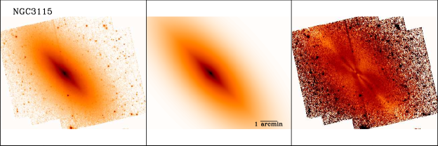
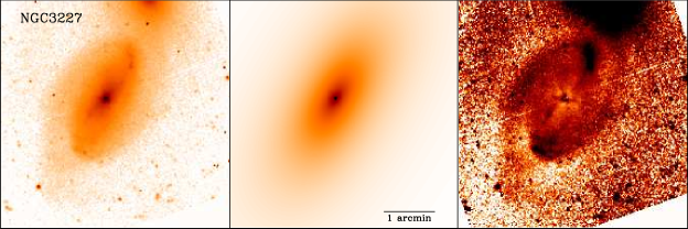
An important issue for bulge decomposition is related to the fitting method. In the case of one dimensional fitting, radially averaged surface brightness profiles are fit with one or more components. Consequently, information related to, e.g., isophotal twists or changes in ellipticity is lost and the galaxy profile is poorly defined. Moreover, in one-dimensional fitting different morphological components may appear to merge smoothly, generating degeneracy and non-uniqueness in the profile decomposition. A two-dimensional analysis breaks this degeneracy (see, e.g., Peng et al. 2002, de Souza, Gadotti & dos Anjos 2004).

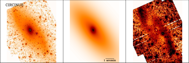
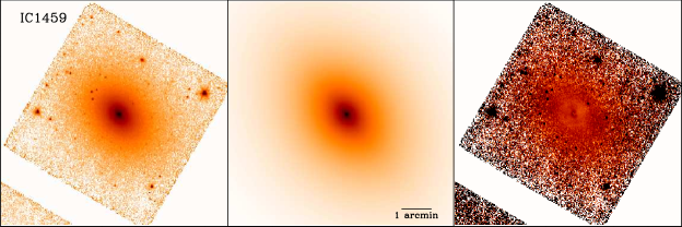
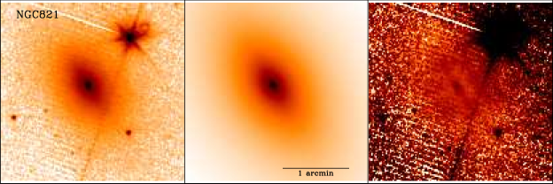
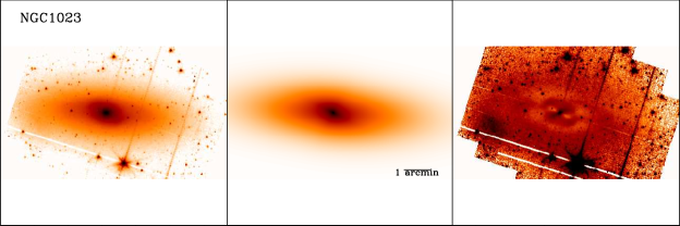
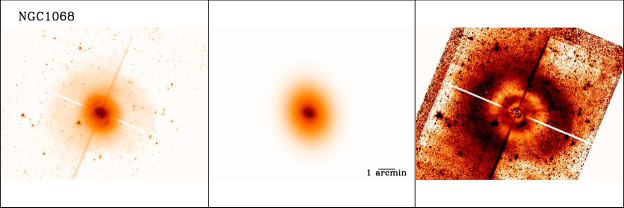
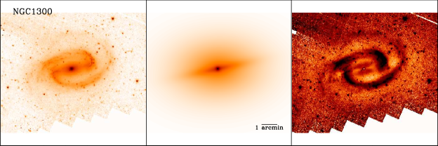
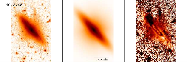
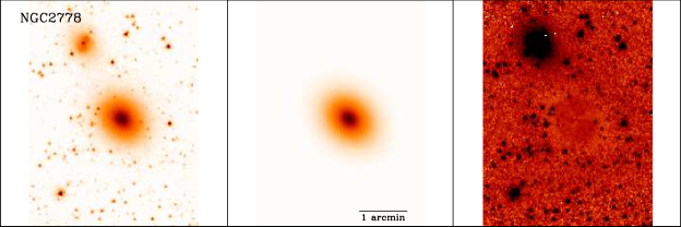
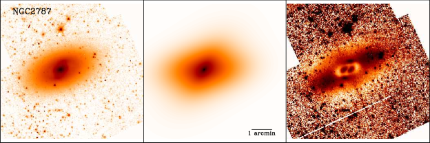
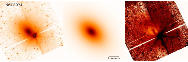
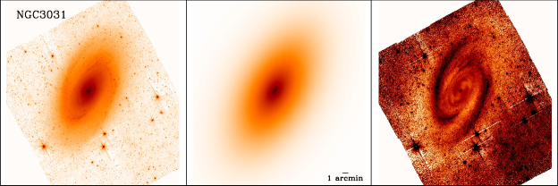
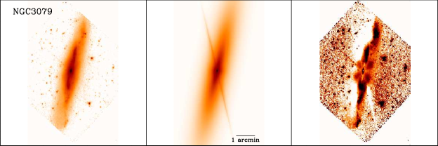
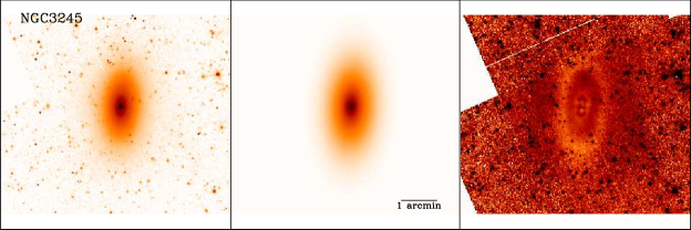
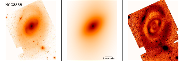
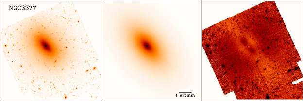
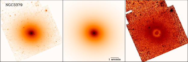
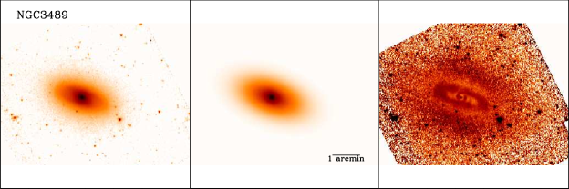
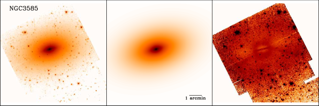
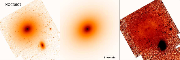
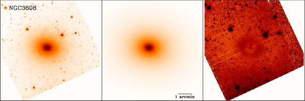
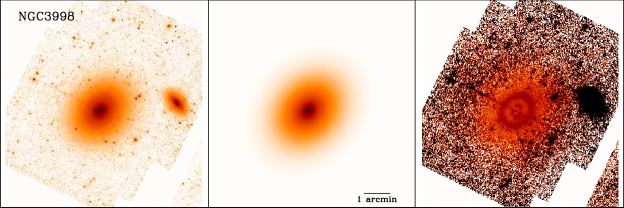
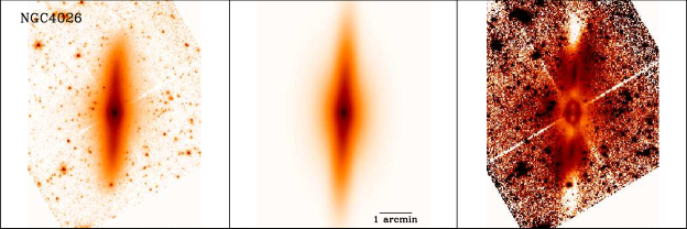
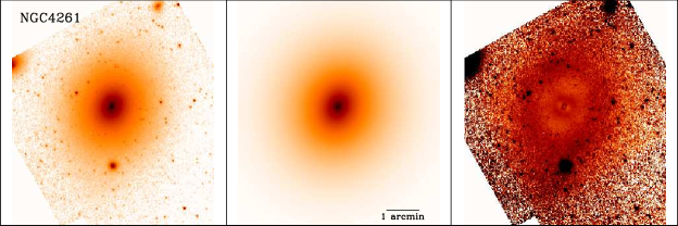
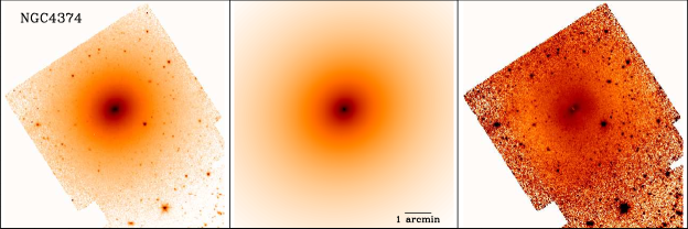
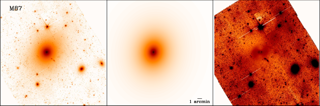
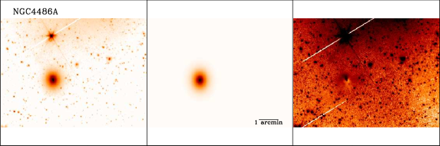
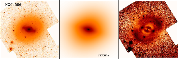
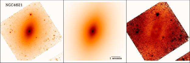
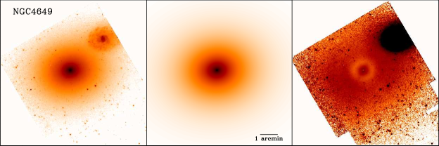
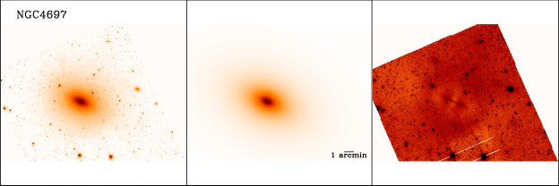
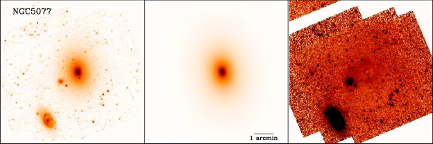
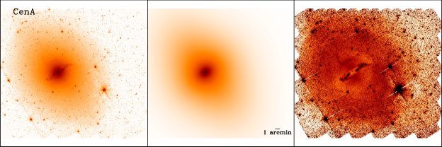
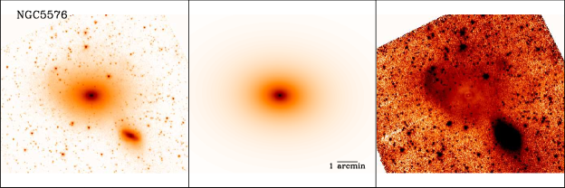
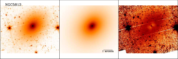
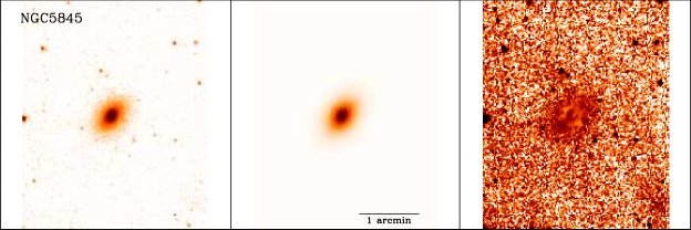
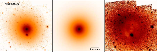
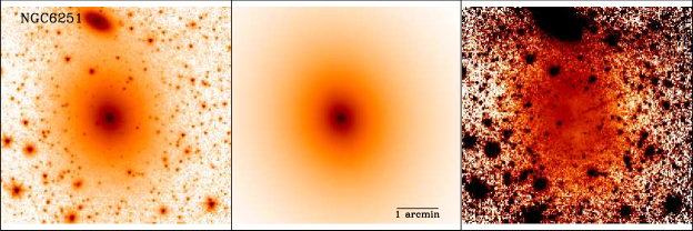
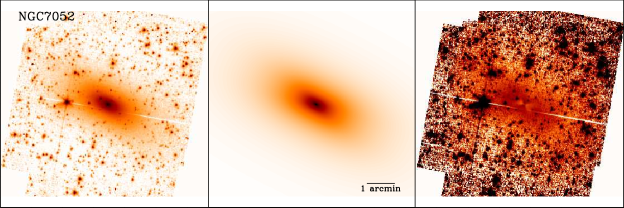
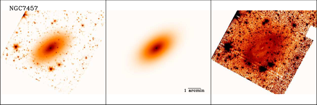
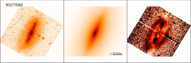
In Section 2.3 we describe in detail our grid method for a two-dimensional decomposition of Spitzer/IRAC 3.6 $\mu$m images. This is an improved version of the two-dimensional method commonly adpted in the literature, where all galaxy parameters are left free to vary. In fact, degeneracies also affect two dimensional methods: one is related to the functional form of the bulge profile, ”Sérsic” profile, in which the $n$ and $R_{\mathrm{e}}$ parameters are strongly coupled. Moreover, the fainter outer parts of galaxies may be affected by errors on background estimates. In Section 2.3 we also justify our choice of the best fit by a quantitative inspection of the $\chi^{2}$ as a function of the radius. We note that the errors on the bulges parameters in Tab. 3 are not one standard deviation errors, rather are given by the discrepancy between the best fit values and the ones obtained from the model having the closest $s,~{}s+\sigma_{s}$ or $s-\sigma_{s}$ value and the lowest possible reduced $\chi^{2}$ within $R^{opt}_{0.5}$ according to the criteria described in Section 2.3. For each galaxy, Fig. 8 shows the image, 2D model, and residuals. It also shows the trend of $\chi^{2}$ vs the source radius for: the best model (i.e. best $n$ in red), the fit for the nearest $n$ with low $\chi^{2}$ within $R^{opt}_{0.5}$ maintaining the same sky values (in dark blue, is plotted to show the dependence on $n$ at small radii), and the model from which we compute the absolute error on free parameters (in sky blue). Even with the above technique when real galaxies are fitted in two dimensions, their surface brightness in the circumnuclear regions is rarely well reproduced only by axisymmetric components. In fact, it is not uncommon to find inner disks and non-axisymmetric features in elliptical galaxies (e.g. Moriondo et al. 1998, Laurikainen et al. 2005). Substructure in the circumnuclear regions of both elliptical and spiral galaxies (such ovals, disks, lenses) occurs frequently, and is usually impossible to fit them with only axisymmetric components, with or without the addition of a bar. This is the origin of nuclear structures in the residual images shown in Fig. 8. Finally, we also note that our models (red curves in Fig. 8) do not require any additional nuclear component to respect the quality criteria of Section 2.3, for which, no more than $5\%$ of the nuclear flux should be lost.

Figure 8: Two-dimensional decomposition.The image, best-fit model and residuals are shown in logarithmic scale. The residuals are stretched ($\pm 0.25$dex) to highlight the finest details. On the right, the $\chi^{2}$ is plotted as a function of the radius (in arcsec). Red: best model. Dark blue: the fit with closest $n$ and the lowest $\chi^{2}$ within $R^{opt}_{0.5}$. Light blue: same for the closest sky ($s\pm\sigma_{s}$, see Section 2.3 and Appendix A for details). A color version of this figure is available online.

Figure 8: Continued.

Figure 8: Continued.

Figure 8: Continued.

Figure 8: Continued.

Figure 8: Continued.

Figure 8: Continued.

Figure 8: Continued.

Figure 9: Continued.

Figure 10: Continued.

Figure 11: Continued.

Figure 12: Continued.

References

- Akritas & Bershady (1996) Akritas M. G., Bershady M. A., 1996, ApJ, 470, 706
- Allen (1976) Allen C. W., 1976, Astrophysical Quantities. Athlone, London
- Aller & Richstone (2007) Aller M. C., Richstone D. O., 2007, ApJ, 665, 120
- Andredakis, Peletier, & Balcells (1995) Andredakis Y. C., Peletier R. F., Balcells M., 1995, MNRAS, 275, 874
- Barway & Kembhavi (2007) Barway S., Kembhavi A., 2007, ApJ, 662, L67
- Batcheldor (2010) Batcheldor D., 2010, ApJ, 711, L108
- Bell & de Jong (2001) Bell E. F., de Jong R. S., 2001, ApJ, 550, 212
- Bell et al. (2003) Bell E. F., McIntosh D. H., Katz N., Weinberg M. D., 2003, ApJS, 149, 289
- Bessell & Brett (1988) Bessell M. S., & Brett J. M. 1988, PASP, 100, 1134
- Burstein et al. (1997) Burstein D., Bender R., Faber S., Nolthenius R., 1997, AJ, 114, 1365
- Cappellari et al. (2006) Cappellari M., et al. 2006, MNRAS, 366, 1126
- Drory, Bender, & Hopp (2004) Drory N., Bender R., Hopp U., 2004, ApJ, 616, L103
- de Souza, Gadotti, & dos Anjos (2004) de Souza R. E., Gadotti D. A., dos Anjos S., 2004, ApJS, 153, 411
- Djorgovski & Davis (1987) Djorgovski S., Davis M., 1987, ApJ, 313, 59
- Erwin (2010) Erwin P. 2010, arXiv:1002.1445
- Fazio et al. (2004) Fazio G. G., et al. 2004, Bulletin of the American Astronomical Society, 36, 699
- Feoli et al. (2010) Feoli A., Mancini L., Marulli F., van den Bergh S., 2010, GReGr, 57
- Ferrarese & Merritt (2000) Ferrarese L., & Merritt D. 2000, ApJ, 539, L9
- Fisher & Drory (2008) Fisher D. B., & Drory N. 2008, AJ, 136, 773
- Fisher & Drory (2010) Fisher D. B., & Drory N. 2010, ApJ, 716, 942
- Gadotti (2009) Gadotti D. A. 2009, MNRAS, 393, 1531
- Gebhardt et al. (2000) Gebhardt K., et al. 2000, ApJ, 539, L13
- Gebhardt et al. (2003) Gebhardt K., et al., 2003, ApJ, 583, 92
- Giovanardi & Hunt (1988) Giovanardi C., Hunt L. K., 1988, AJ, 95, 408
- Graham (2007) Graham, A. W. 2007, MNRAS, 379, 711
- Graham (2008) Graham A. W. 2008a, Publications of the Astronomical Society of Australia, 25, 167
- Graham (2008) Graham A. W., 2008b, ApJ, 680, 143
- Graham & Li (2009) Graham A. W., Li I.-h., 2009, ApJ, 698, 812
- Graham & Spitler (2009) Graham A. W., & Spitler L. R. 2009, MNRAS, 397, 2148
- Greene et al. (2008) Greene J. E., Ho L. C., & Barth A. J. 2008, ApJ, 688, 159
- Gültekin et al. (2009) Gültekin K., et al. 2009, ApJ, 698, 198
- Häring & Rix (2004) Häring N., & Rix H.-W. 2004, ApJ, 604, L89
- Helou et al. (2004) Helou G., et al., 2004, ApJS, 154, 253
- Hopkins et al. (2007) Hopkins P. F., Hernquist L., Cox T. J., Robertson B., & Krause E. 2007, ApJ, 669, 67
- Hu (2009) Hu J. 2009, arXiv:0908.2028
- Hunt et al. (2004) Hunt L. K., Pierini D., & Giovanardi C. 2004, A&A, 414, 905
- Kelly (2007) Kelly B. C. 2007, ApJ, 665, 1489
- Kormendy Richstone (1995) Kormendy J., & Richstone D. 1995, ARA&A, 33, 581
- Kormendy & Kennicutt (2004) Kormendy J., & Kennicutt R. C., Jr. 2004, ARA&A, 42, 603
- Jorgensen, Franx, & Kjaergaard (1996) Jorgensen I., Franx M., Kjaergaard P., 1996, MNRAS, 280, 167
- Jun & Im (2008) Jun H. D., & Im M. 2008, ApJ, 678, L97
- Labita et al. (2009) Labita M., Decarli R., Treves A., Falomo R., 2009, MNRAS, 399, 2099
- Lamastra et al. (2010) Lamastra A., Menci N., Maiolino R., Fiore F., & Merloni A. 2010, MNRAS, 405, 29
- Leitherer et al. (1999) Leitherer C., et al., 1999, ApJS, 123, 3
- Lauer et al. (2007) Lauer T. R., et al. 2007, ApJ, 662, 808
- Laurikainen et al. (2009) Laurikainen E., Salo H., Buta R., & Knapen J. H. 2009, ApJ, 692, L34
- Magorrian et al. (1998) Magorrian J., et al., 1998, AJ, 115, 2285
- Merloni et al. (2010) Merloni A., et al. 2010, ApJ, 708, 137
- Makovoz & Marleau (2005) Makovoz D., & Marleau F. R. 2005, PASP, 117, 1113
- Marconi & Hunt (2003) Marconi A., & Hunt L. K. 2003, ApJ, 589, L21
- Marconi et al. (2004) Marconi A., Risaliti G., Gilli R., Hunt L. K., Maiolino R., & Salvati, M. 2004, MNRAS, 351, 169
- Moriondo, Giovanardi, & Hunt (1998) Moriondo G., Giovanardi C., Hunt L. K., 1998, A&AS, 130, 81
- Nowak et al. (2010) Nowak N., Thomas J., Erwin P., Saglia R. P., Bender R., Davies R. I., 2010, MNRAS, 403, 646
- Padmanabhan et al. (2004) Padmanabhan N., et al., 2004, NewA, 9, 329
- Peng et al. (2002) Peng C. Y., Ho L. C., Impey C. D., Rix H.-W., 2002, AJ, 124, 266
- Peng et al. (2006) Peng C. Y., Impey C. D., Rix H.-W., Kochanek C. S., Keeton C. R., Falco E. E., Lehár J., McLeod B. A., 2006, ApJ, 649, 616
- Peng et al. (2007) Peng C. Y., Ho L. C., Impey C. D., Rix H. W., 2007, AAS, 38, 804
- Prugniel & Simien (1996) Prugniel P., Simien F., 1996, A&A, 309, 749
- Reach et al. (2005) Reach W. T., et al., 2005, PASP, 117, 978
- Shankar (2009) Shankar F., 2009, NewAR, 53, 57
- Shen et al. (2008) Shen Y., Greene J. E., Strauss M. A., Richards G. T., Schneider D. P., 2008, ApJ, 680, 169
- Shields et al. (2003) Shields G. A., Gebhardt K., Salviander S., Wills B. J., Xie B., Brotherton M. S., Yuan J., Dietrich M., 2003, ApJ, 583, 124
- Soltan (1982) Soltan A., 1982, MNRAS, 200, 115
- Trakhtenbrot & Netzer (2010) Trakhtenbrot B., & Netzer H. 2010, MNRAS, L76
- Tremaine et al. (2002) Tremaine S., et al. 2002, ApJ, 574, 740
- Woo et al. (2008) Woo J.-H., Treu T., Malkan M. A., Blandford R. D., 2008, ApJ, 681, 925