Multidimensional Modeling of Type I X-ray Bursts. I. Two-Dimensional Convection Prior to the Outburst of a Pure ⁴He Accretor

Abstract

We present multidimensional simulations of the early convective phase preceding ignition in a Type I X-ray burst using the low Mach number hydrodynamics code, MAESTRO. A low Mach number approach is necessary in order to perform long-time integration required to study such phenomena. Using MAESTRO, we are able to capture the expansion of the atmosphere due to large-scale heating while capturing local compressibility effects such as those due to reactions and thermal diffusion. We also discuss the preparation of one-dimensional initial models and the subsequent mapping into our multidimensional framework. Our method of initial model generation differs from that used in previous multidimensional studies, which evolved a system through multiple bursts in one dimension before mapping onto a multidimensional grid. In our multidimensional simulations, we find that the resolution necessary to properly resolve the burning layer is an order of magnitude greater than that used in the earlier studies mentioned above. We characterize the convective patterns that form and discuss their resulting influence on the state of the convective region, which is important in modeling the outburst itself.

1 Introduction

Type I X-ray bursts are possibly the most frequent thermonuclear explosions in the universe and provide a large amount of observational data that can be used to determine the properties of matter near the surface of a neutron star. To make meaningful inferences about these properties from observational data, however, we must have a proper theoretical understanding of the bursting phenomena (Bhattacharyya, 2010). The basic XRB paradigm takes place in a mass-transferring, low-mass X-ray binary (LMXB) system in which the neutron star’s companion has filled its Roche lobe and is dumping H- and/or He-rich material onto the surface of the neutron star. Depending on the accretion rate and composition, there are several burning regimes that will trigger an XRB (see Bildsten (2000) for an overview). The general idea is that a column of accreted material—or heavier-element ash from prior stable burning of accreted material—builds up until the temperature sensitivity of the energy generation rate at the base of the layer exceeds that of the local cooling rate and a thin-shell thermal instability forms. The instability eventually causes a runaway of unstable burning resulting in an outburst.

One-dimensional hydrodynamic studies reproduce many of the observable features of XRBs such as burst energies ($\sim 10^{39}$ erg), rise times (seconds), durations ($10$’s – $100$’s of seconds) and recurrence times (hours to days) (Woosley & Weaver, 1984; Taam et al., 1993; Heger et al., 2007a; also see Strohmayer & Bildsten (2006) for a review of XRBs). By construction, however, one-dimensional models assume that the fuel is burned uniformly over the surface of the star, which is highly unlikely given the large disparity between the thermalization and burning timescales of the accreted material (Shara, 1982). Furthermore, the Rossi X-ray Timing Explorer satellite has observed coherent oscillations in the lightcurves of $\sim 20$ outbursts from LMXB systems (first by Strohmayer et al., 1996; more recently by Altamirano et al., 2010 and references therein). The asymptotic evolution of the frequency of such oscillations suggests they are modulated by the neutron star spin frequency (Muno et al., 2002). Oscillations observed during the rising portion of an outburst lightcurve are therefore indicative of a spreading burning front being brought in and out of view by stellar rotation. Additionally, oscillations observed during the decay phase of the burst are thought to be caused by unstable surface modes that may depend critically on the local heating and cooling rates during the burst (Narayan & Cooper, 2007, and references therein). The manner in which the burning front spreads and propagates throughout the accreted atmosphere is not well known, and a proper multidimensional modeling of the conditions in the atmosphere prior to outburst is needed (e.g. Fryxell & Woosley, 1982b).

Prior to the actual outburst, the burning at the base of the ignition column drives convection throughout the overlying layers and determines the state of the material in which the burning front will propagate. One-dimensional simulations of XRBs usually attempt to parameterize the convective overturn and mixing using astrophysical mixing-length theory (Böhm-Vitense, 1958) or through various diffusive processes (see Heger et al. 2000 for a thorough discussion). Recent multidimensional simulations of stellar convection (see Arnett et al., 2009, and references therein), however, show a large discrepancy in, for example, the velocity of a typical convective eddy when compared to one-dimensional models in the case of stellar evolution codes that use mixing-length theory. Indeed, there has recently been an effort put forth in the astrophysical community, the so-called Convection Algorithms Based on Simulations, or CABS, to derive from multidimensional simulations a more physically motivated prescription for handling convection in one dimension (Arnett et al., 2008). To date, such methods have not propagated into the XRB-simulation community and a proper treatment of convection, without assumptions, requires simulation in multiple dimensions.

Multidimensional simulations of any aspect of XRBs, however, have hitherto been rather restrictive. A burning front can propagate either supersonically as a detonation or subsonically as a deflagration. Full hydrodynamic XRB detonation models in the spirit of Fryxell & Woosley (1982a) or Zingale et al. (2001) require a thick ($\sim 100$ m) accreted helium layer. Such deep layers are only produced by very low accretion rates, which are inconsistent with the majority of rates inferred from observations of XRBs, and therefore the burning front in most XRBs likely propagates as a deflagration. Deflagration models are difficult to compute with standard compressible hydrodynamics codes due to the long integration times required. One possible solution is to eliminate the effect of acoustic waves in the system, allowing the time step to be controlled by the fluid velocity, rather than the sound speed. Such a method can be derived using low Mach number asymptotics; classic examples of low Mach number approaches include the incompressible, anelastic (Ogura & Phillips, 1962) and Boussinesq (Boussinesq, 1903) approximations. To this end, Spitkovsky et al. (2002) used a simple, shallow-water, 2-layer, incompressible fluid to model the vertical structure of a deflagration front and showed how rotation coupled with convection may play an important role in regulating the spread of the front over the surface of the neutron star.

More recently, Lin et al. (2006) developed and applied a low Mach number approximation method to the problem of convective burning at the base of an accreted layer in an XRB system. Their method, however, was first order accurate in space and time and did not allow for the evolution of the hydrostatic base state, a feature that is needed to capture the expansion of the atmosphere in response to heating. Furthermore, Lin et al. did not model the surface of the accreted layer, which is vital to understanding bursts that exhibit photospheric radius expansion (PRE bursts); such bursts are crucial in determining the stellar properties of neutron stars (Steiner et al., 2010, and references therein).

In this study we use MAESTRO (Nonaka et al., 2010), a multidimensional low Mach number hydrodynamics algorithm for astrophysical flows, to model the convection leading up to an outburst of a pure ⁴He accretor. MAESTRO is a second-order accurate, conservative method that uses rectangular grid cells. The algorithm is capable of capturing the expansion of the atmosphere due to large-scale heating, while capturing local compressibility effects due to reactions, thermal diffusion and compositional changes. A semi-analytic method is used to generate one-dimensional initial models. These models are then augmented by being evolved in a one-dimensional stellar evolution code; this evolution allows for the approximation of the convective cooling and leads to a model that is closer to satisfying the thin shell instability condition. The resulting model is then mapped into MAESTRO and evolved in multiple dimensions.

The main goals of this paper are to explore and describe the challenges of modeling XRBs in multiple dimensions and to better understand the convective phase that precedes the outburst. The remainder of this paper is as follows. In Section 2, we describe the generation of the initial models and the subsequent mapping into a multidimensional framework. In Section 3, we describe the MAESTRO algorithm, including the addition of two new modules not present in the original algorithm. Specifically, we have added thermal conduction and a “volume discrepancy” correction term to the velocity field to ensure that the solution does not diverge from the equation of state. In Section 4, we describe the results of our multidimensional simulations. In particular we discuss the resolution needed to properly resolve the burning layer, the effects of including the thermal diffusion and volume discrepancy correction terms, the expansion of the base state due to heating and finally the nature of the convective behavior and its effect on the atmosphere. We conclude in Section 5 by summarizing our results and describing our plans to extend the current study to mixed H/He XRB sources.

2 Initial Models

We begin our calculations by generating a one-dimensional initial model of the accreted layer in hydrostatic (HSE) and thermal equilibria on the surface of a neutron star. We assume a plane-parallel geometry—that is, the gravitational acceleration, $g$, is assumed constant throughout the domain, which is justified because the thickness of the accreted layer ($\sim 10$ m) is much less than the radius of the neutron star ($\sim 10$ km). We assume a ⁴He layer is accreted on top of a ⁵⁶Fe neutron star with a trace abundance ($10^{-10}$) of ¹²C. We choose a pure ⁴He accretor both because the corresponding nuclear reaction network, $3\alpha$ burning, is simple compared to the slow, $\beta$-decay-limited burning processes in bursts involving H, and because ultra-compact XRB sources are possible pure ⁴He accretors (4U 1820-30, for example; Cumming 2003). We include the forward and reverse $3\alpha$ reaction rates as given in Caughlan & Fowler (1988) with electron screening contributions from Graboske et al. (1973) for the weak regime and from Alastuey & Jancovici (1978) for the strong regime.

There are several approaches to one-dimensional model generation in the literature. In our approach, we begin with a semi-analytic initial model and then augment the model to account for convective cooling. We also discuss proper mapping of the one-dimensional model to our multidimensional framework.

2.1 Semi-Analytic Models

The semi-analytic approach to model generation involves integration of the heat equation and an entropy equation,

$$\frac{dT}{dy} = \frac{3\kappa F}{4acT^{3}}$$ (1)

$$\frac{dF}{dy} = 0,$$ (2)

where $c$ is the speed of light, $a$ the radiation constant, $\kappa$ the opacity (including radiative and conductive contributions), $T$ the temperature, $F$ the outward heat flux and $dy=-\rho dr$ with $y(r)$ the column-depth (see Cumming & Bildsten 2000 for details of this method). Note that (1) can give a thermal profile that is superadiabatic—in practice, the thermal gradient is restricted to be $dT/dy\leq\left(dT/dy\right)_{s}$ where the subscript $s$ means along an adiabat. Also note that for simplicity, equation (2) neglects any compressional heating contributions from the accretion itself and assumes the accreted material is not burning during the accretion phase—this is a steady-state configuration. There is, however, an outward heat flux from pycnonuclear reactions deep within the neutron star crust; we approximate this flux as a constant value throughout the accreted layer, $F=200$ keV per nucleon. The integration starts at the top of the ⁴He atmosphere (arbitrarily at $y_{\text{top}}=10^{3}$ g cm^-2) where a radiative zero solution is assumed, and continues until the thin shell instability condition (Fushiki & Lamb, 1987),

$$\frac{d\epsilon_{3\alpha}}{dT}>\frac{d\epsilon_{\text{cool}}}{dT},$$ (3)

is reached at $y=y_{\text{base}}$. The local cooling rate is typically approximated from (1) and (2) as

$$\epsilon_{\text{cool}}\approx\frac{acT^{4}}{3\kappa y^{2}}.$$ (4)

When (3) is attained, the composition for $y>y_{\text{base}}$ is switched to ⁵⁶Fe  and integration of (1) and (2) resumes until a thick enough substrate is formed such that $y_{\text{base}}$ is sufficiently far from the bottom of the computational domain, $y(r=0)=10^{12}$ g cm^-2 in our studies.

The approximation, (4), works well in one dimension because the only efficient way the system can cool (neglecting weak reactions) is via conduction and radiation, which enter through the opacity. When more spatial dimensions are added to the system and there is heating from below from nuclear reactions, the fluid is free to overturn and cool via convection. Now we have a situation where the local multidimensional cooling rate, $\epsilon_{\text{cool, multi-d}}=\epsilon_{\text{cool}}+\epsilon_{\text{conv}}$, exceeds the initial approximation and (3) may no longer be satisfied. Therefore, such a semi-analytic model is no longer close to runaway and to evolve the system in multiple dimensions until (3) is reached is intractable even with the advantages of a low Mach number approximation code.

2.2 Kepler-supplemented Models

One way to overcome the difficulties with evolving the model described in the previous section in multiple dimensions is to explicitly include an effective convective cooling term in the approximation to the local cooling given by equation (4). This effective convective cooling can be included via mixing-length theory typically found in stellar evolution codes. Using the semi-analytic model described above as initial conditions, the one-dimensional stellar evolution code, Kepler (Weaver et al., 1978), was used to construct the remainder of the underlying neutron star with $R_{\text{ns}}=10$ km and $M_{\text{ns}}=1.87M_{\odot}$ (Woosley, 2010; private communication). The system is then allowed to evolve in one dimension whereupon nuclear burning heats the base of the layer, and the convection prescription develops a well-mixed and nearly adiabatic region of ¹²C ash overlying the ⁴He base. This results in a model that is much closer to satisfying the thermal instability criterion, (3), when mapped into multiple dimensions.

2.3 Mapping to Multiple Dimensions

The data from Kepler are given in a Lagrangian (mass) coordinate system and we need to convert them to an Eulerian (physical) coordinate system for use in MAESTRO. We use a procedure similar to that found in Zingale et al. (2002) to ensure our initial model is in HSE. Given the density, temperature and composition from the Kepler evolution, we call the equation of state to get the pressure. We then discretize the HSE equation and solve for the non-uniform Eulerian grid spacing corresponding to the Lagrangian grid points,

$$r_{i}=r_{i-1}-\frac{1}{g}\frac{p_{i}-p_{i-1}}{\mathchoice{\kern 0.0pt\raise 2.15277pt\hbox{\sevenrm1}\kern-1.49994pt/\kern-1.49994pt\lower 1.07639pt\hbox{\sevenrm2}}{\kern 0.0pt\raise 2.15277pt\hbox{\sevenrm1}\kern-1.49994pt/\kern-1.49994pt\lower 1.07639pt\hbox{\sevenrm2}}{\kern 0.0pt\raise 2.15277pt\hbox{\fiverm1}\kern-1.99997pt/\kern-1.49994pt\lower 1.07639pt\hbox{\fiverm2}}{1\!/2}\left(\rho_{i}+\rho_{i-1}\right)},$$ (5)

where $r$ is the radial coordinate, $p$ the pressure and $\rho$ the density. We set $r_{1}=0$ to complete the description of the grid. The transition from the pure ⁵⁶Fe neutron star (at $r_{\text{trans}}$) to the ⁴He atmosphere (at $r_{\text{trans}+1}$) is a step function as a result of the initial Lagrangian data. Such sharp transitions can be a source of numerical noise and oscillations as the solution evolves on an Eulerian grid. To minimize the numerical noise, we smooth the interface by adding $n$ uniformly distributed coordinate points between $r_{\text{trans}}$ and $r_{\text{trans}+1}$. The temperature at these new points is linearly interpolated between $T_{\text{trans}}$ and $T_{\text{trans}+1}$. Then $X(\text{${}^{4}$He})$ and $X(\text{${}^{12}$C})$ at the new points are filled with a $\tanh$ profile:

$$\phi_{i}=\alpha\tanh\left(\frac{r_{i}-r_{\text{c}}}{\varphi}\right)+\phi_{\text{c}}$$ (6)

where $\alpha=\left(\phi_{\text{trans}+1}-\phi_{\text{trans}}\right)/2$, $r_{\text{c}}=\left(r_{\text{trans}}+r_{\text{trans}+1}\right)/2$, $\phi_{\text{c}}=\left(\phi_{\text{trans}}+\phi_{\text{trans}+1}\right)/2$ and $\varphi$ is a parameter to set the smoothness. $X(\text{${}^{56}$Fe})$ is then found from the constraint $\sum_{k}X_{k}=1$, and $p$ and $\rho$ are found by using an iterative Newton-Raphson technique with the equation of state and (5) at these new points. This smoothed model is then linearly interpolated onto a completely uniform grid, with $r_{i}=r_{i-1}+\Delta r$, and is again put into HSE using (5) and the equation of state. Values of $n=50$ and $\varphi=3$ were used to smooth the models presented in this work.

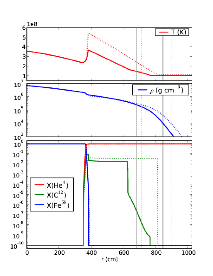
Figure 1 shows the result of this procedure for two models that were evolved in Kepler until the base of the ⁴He atmosphere had reached a temperature of $3.67\times 10^{8}$ K (solid line, hereafter referred to as the cold model) and $5.39\times 10^{8}$ K (dotted line, hereafter referred to as the hot model). The density at the base of the ⁴He layer for the cold model is $1.4\times 10^{6}$ g cm^-3 and is $1.2\times 10^{6}$ g cm^-3 for the hot model. For comparison, the initial model of Lin et al. (2006) had a base temperature and density of $2\times 10^{8}$ K and $4\times 10^{6}$ g cm^-3, respectively. The cold model has a peak in ¹²C production around $r=382$ cm (i.e., the base of the ⁴He layer in both models) that appears smoothed in the more evolved hot model. Both models, however, have an extended region of well-mixed ¹²C that extends to $r=624$ cm ($r=812$ cm) for the cold (hot) model. These initial models contain no multidimensional velocity information from the Kepler simulations. We therefore make no assumptions about the nature of the convection when the models are mapped into multiple dimensions in MAESTRO.

3 Hydrodynamics Algorithm

For our multidimensional simulations, we use the low Mach number stellar hydrodynamics algorithm, MAESTRO. This code is appropriate for flows in the low Mach number regime, where the characteristic fluid velocity is small compared to the speed of sound. Note that the algorithm does not enforce that the Mach number remain small, but rather is only valid for such flows. A series of papers (see Almgren et al. (2006a)—henceforth Paper I, Almgren et al. (2006b)—henceforth Paper II, Almgren et al. (2008)—henceforth Paper III, and Zingale et al. (2009)—henceforth Paper IV) describe the derivation of the low Mach number equation set, its algorithmic implementation, and the initial application to convection in a white dwarf preceding a Type Ia supernova. We use the most recent version of the algorithm, which includes local adaptive mesh refinement, as given in Nonaka et al. (2010)—henceforth Paper V.

One key advantage of using a low Mach number approach is the increase of allowable time step size, which enables long-time integration. Standard compressible hydrodynamics codes for astrophysical applications such as CASTRO (Almgren et al., 2010) or FLASH (Fryxell et al., 2000) evolve a fully compressible equation set, i.e., the Euler equations, which allows for the formation and propagation of shocks. For low speed convective motion in our pre-burst convection studies, we do not need to explicitly follow the propagation of sound waves. Our low Mach number equation set does not contain acoustic waves, and therefore MAESTRO is able to take time steps constrained by the maximum fluid velocity, rather than the maximum sound speed. As an example, if the maximum Mach number of the flow is $M\sim 0.01$, we will obtain a factor of $1/M\sim 100$ increase in time step size compared to a standard compressible approach. Another advantage of a low Mach number method is that the overall HSE of the state can be guaranteed by the inclusion of a base state in HSE in the low Mach number equation set. This removes the difficulties of maintaining HSE commonly found in compressible hydrodynamics codes.

MAESTRO solves a system of advection-reaction-diffusion equations with the equation of state formulated as an elliptic constraint on the velocity. MAESTRO uses a higher-order Godunov method to discretize the advective terms, Strang-splitting to couple the reaction terms to the advective terms, and a semi-implicit treatment of the diffusion terms. The diffusion term and the divergence constraint are formulated as linear systems which are solved iteratively using multigrid. The evolution of the one-dimensional base state density is also computed. The base state density represents the average state of the atmosphere, and is coupled to the base state pressure via HSE. The base state density has its own evolution equation that computes the expansion of the atmosphere due to heating and is discretized using a higher-order Godunov method. We note that MAESTRO is second-order accurate in space and time.

3.1 MAESTRO Details

We now provide additional details of the low Mach number equation set and numerical implementation. The interested reader is referred to Papers I-V for full details. We use a two-dimensional Cartesian formulation with $x$ the horizontal coordinate and $r$ the radial coordinate. The low Mach number equation set is:

$$\frac{\partial(\rho X_{k})}{\partial t} = -\mathbf{\nabla}\cdot(\rho X_{k}\boldsymbol{U})+\rho\dot{\omega}_{k},$$ (7)

$$\frac{\partial\boldsymbol{U}}{\partial t} = -\boldsymbol{U}\cdot\mathbf{\nabla}\boldsymbol{U}-\frac{1}{\rho}\mathbf{\nabla}\pi-\frac{(\rho-\rho_{0})}{\rho}g\boldsymbol{e}_{r},$$ (8)

$$\frac{\partial(\rho h)}{\partial t} = -\mathbf{\nabla}\cdot(\rho h\boldsymbol{U})+\frac{Dp_{0}}{Dt}+\rho H_{\rm nuc}+\mathbf{\nabla}\cdot(k_{\rm th}\mathbf{\nabla}T),$$ (9)

where $\boldsymbol{U}$, $h$ and $k_{\rm th}$ are the velocity, specific enthalpy, and thermal conductivity, respectively. The species are represented by their mass fractions, $X_{k}$, along with their associated production rates, $\dot{\omega}_{k}$, and $H_{\rm nuc}$ is the nuclear energy generation rate per unit mass. Using low Mach number asymptotics (see Paper I) the total pressure, $p(x,r,t)$, is decomposed into a base state pressure, $p_{0}(r,t)$, and a perturbational, or dynamic, pressure, $\pi(x,r,t)$, such that $|\pi|/p_{0}=\mathcal{O}(M^{2})$. The base state density, $\rho_{0}(r,t)$, is in HSE with the base state pressure such that $\mathbf{\nabla}p_{0}=-\rho_{0}g\boldsymbol{e}_{r}$, where $\boldsymbol{e}_{r}$ is the unit vector in the outward radial direction.

Thermal conduction was not present in Paper V, so we have developed a semi-implicit discretization for this term. We include full algorithmic implementation details in Appendix A and a verification test problem in Appendix A.1.

Mathematically, this system must still be closed by the equation of state, which is expressed as a divergence constraint on the velocity field (see Paper III),

$$\mathbf{\nabla}\cdot(\beta_{0}\boldsymbol{U})=\beta_{0}\left(S-\frac{1}{\overline{\Gamma}_{1}p_{0}}\frac{\partial p_{0}}{\partial t}\right),$$ (10)

where $\beta_{0}$ is a density-like variable,

$$\beta_{0}(r,t)=\rho(0,t)\exp\left({\int_{0}^{r}\frac{1}{\overline{\Gamma}_{1}p_{0}}\frac{\partial p_{0}}{\partial r^{\prime}}\;dr^{\prime}}\right),$$ (11)

and $\overline{\Gamma}_{1}(r)$ is the average of $\Gamma_{1}=\left(d\ln p/d\ln\rho\right)_{s}$ where the subscript $s$ means the derivative is taken at constant entropy. We will use an overline notation to represent the average of a quantity, which computationally is the arithmetic average of all grid cells at a particular radius. The expansion term, $S$, in (10) accounts for local compressibility effects resulting from nuclear burning, compositional changes, and thermal conduction:

$$S = \sigma H_{\rm nuc}+-\sigma\sum_{k}\xi_{k}\dot{\omega}_{k}+\frac{1}{\rho p_{\rho}}\sum_{k}p_{X_{k}}\dot{\omega}_{k}+\frac{\sigma}{\rho}\mathbf{\nabla}\cdot(k_{\rm th}\mathbf{\nabla}T),$$ (12)

where $\xi_{k}\equiv\left(\partial h/\partial X_{k}\right)_{\rho,T,(X_{j},j\neq k)}$, $p_{\rho}\equiv\left(\partial p/\partial\rho\right)_{T,X_{k}}$, $p_{X_{k}}\equiv\left(\partial p/\partial X_{k}\right)_{T,\rho,(X_{j},j\neq k)}$ and $\sigma\equiv p_{T}/(\rho c_{p}p_{\rho})$ with $p_{T}\equiv\left(\partial p/\partial T\right)_{\rho,X_{k}}$, and $c_{p}\equiv\left(\partial h/\partial T\right)_{p,X_{k}}$.

Another addition to the MAESTRO algorithm is the use of a “volume discrepancy” correction. Because (10) is a linearization of the nonlinear constraint imposed by the equation of state, the thermodynamic pressure, $p_{\text{EOS}}=p(\rho,h,X_{k})$, may drift from the base state pressure, $p_{0}$, (Pember et al., 1998). To correct for this drift, (10) is augmented with a term that drives the thermodynamic pressure back to the that of the base state:

$$\mathbf{\nabla}\cdot(\beta_{0}\boldsymbol{U})=\beta_{0}\left(S-\frac{1}{\overline{\Gamma}_{1}p_{0}}\frac{\partial p_{0}}{\partial t}-\frac{f}{\overline{\Gamma}_{1}p_{0}}\frac{p_{0}-p_{\text{EOS}}}{\Delta t}\right),$$ (13)

where $f$ is the volume discrepancy correction factor and $0\leq f\leq 1$. In Section 4.4, we explore the effectiveness of this term at keeping the overall solution in thermodynamic equilibrium.

To track the evolution of the base state density, we first define the expansion velocity as the average outward velocity:

$$w_{0}(r,t)=\overline{(\boldsymbol{U}\cdot\boldsymbol{e}_{r})}.$$ (14)

As described in Paper V, we compute $w_{0}$ by integrating a one-dimensional divergence constraint, found by taking the average of equation (13):

$$\frac{\partial\left(\beta_{0}w_{0}\right)}{\partial r}=\beta_{0}\left(\overline{S}-\frac{1}{\overline{\Gamma}_{1}p_{0}}\frac{\partial p_{0}}{\partial t}-\frac{f}{\overline{\Gamma}_{1}p_{0}}\frac{p_{0}-\overline{p_{\text{EOS}}}}{\Delta t}\right).$$ (15)

The evolution equation for the base state density can be found by considering the average of the continuity equation:

$$\frac{\partial\rho_{0}}{\partial t}=-\nabla\cdot(\rho_{0}w_{0}\boldsymbol{e}_{r}),$$ (16)

which we discretize with a higher-order Godunov method.

We use special care in dealing with the low density region of our simulation. The density spans many orders of magnitude, and due to conservation of momentum we may generate large velocities in the upper atmosphere that do not affect the solution in the higher-density region. Unfortunately, these large velocities reduce the efficiency of our method by reducing the time step size. The first technique we use to address this problem is the use of a cutoff density, $\rho_{\rm cutoff}$, which is the value we hold the density to outside the star. The second technique we use is the use of an anelastic cutoff density, $\rho_{\rm anelastic}$, below which we determine $\beta_{0}$ by keeping the ratio $\beta_{0}/\rho_{0}$ constant in the divergence constraint in order to minimize spurious wave generation. Full implementation details for the cutoff densities are described in Appendix A.5 of Paper V. In this paper, we use $\rho_{\rm cutoff}=\rho_{\rm anelastic}=10^{4}\text{\ g/cm}^{3}$.

The third technique adopted for the low density region is sponging (or damping), which is used to reduce gravity waves at the surface of the star. This technique is commonly used in the atmospheric modeling community as lateral boundary conditions of limited area simulations (see, for example, Kesel & Winninghoff 1972; Perkey & Kreitzberg 1976) as well as upper boundary conditions to reduce wave reflection off of sharp gradients in the atmospheric structure (see, for example, Durran & Klemp 1983; Durran 1990; Chen et al. 2005). In addition, we have previously utilized the sponging technique in the study of convection in the cores of white dwarfs (Paper IV). Full details for the sponge implementation in MAESTRO can be found in Papers III and IV, but in summary, we add a forcing term to the velocity, which effectively damps the velocity so that $\boldsymbol{U}^{\text{new}}\to\boldsymbol{U}^{\text{new}}*f_{\text{damp}}$. We use the following formulation for the sponge:

$$f_{\text{damp}}=\left\{\begin{array}[]{ll}1,&r\leq r_{\rm sp},\\ \vskip 6.0pt plus 2.0pt minus 2.0pt\cr\frac{1}{2}\left(1-f_{\rm damp,min}\right)\cos\left[\pi\left(\frac{r-r_{\rm sp}}{r_{\rm tp}-r_{\rm sp}}\right)\right]+\frac{1}{2}\left(1+f_{\rm damp,min}\right),&r_{\rm sp}<r\leq r_{\rm tp},\\ \vskip 6.0pt plus 2.0pt minus 2.0pt\cr f_{\rm damp,min},&r_{\rm tp}<r,\end{array}\right.$$ (17)

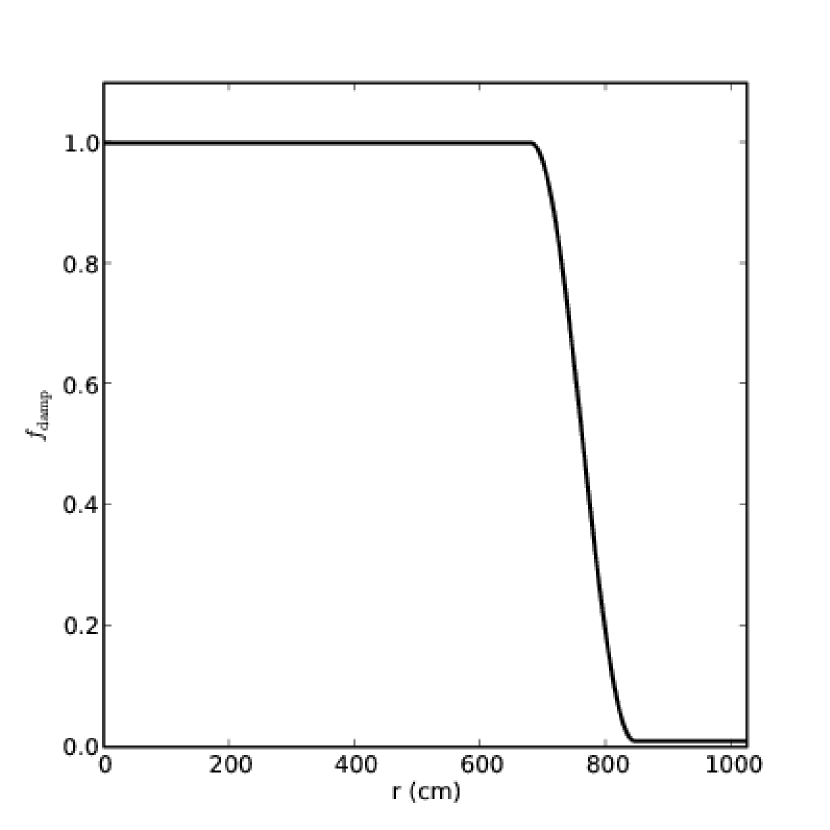
where in our simulations $r_{\rm sp}$ is the radius at which $\rho_{0}=25\rho_{\rm cutoff}$, $r_{\rm tp}$ is the radius at which $\rho_{0}=\rho_{\rm cutoff}$, and $f_{\rm damp,min}=0.01$. In Figure 1, the vertical grey lines correspond to the location of $r_{\rm sp}$ and the vertical black lines correspond to the location of $r_{\rm tp}$ for each of the initial models. Figure 2 shows the initial profile of the sponge for the cold model. Note that as the system evolves it is free to expand thus changing the location of the density cutoffs and consequently the location and extent of the sponge. The inclusion of a sponge layer does not strictly conserve kinetic energy in the sponged region. We note, however, that the material above the surface of the star is at relatively low density compared to the material in the convective region, and therefore the total amount of energy non-conservation is small. Furthermore, as shown in Figure 4 of Paper III, the inclusion of a sponge layer in the low density region of a simulation does not affect the dynamics of the flow in the convective region of interest.

4 Results

We describe below the results of mapping the Kepler-supplemented models into MAESTRO in two dimensions, ($x,\ r$), and the system’s subsequent evolution. Section 4.1 describes the resolution requirements needed to properly resolve the burning layer. In Section 4.2 we show how the inclusion of thermal diffusion affects the nuclear burning layer and its location. We show in Section 4.3 how utilizing a time-dependent base state allows us to capture the expansion of the atmosphere due to heating. Section 4.4 shows how including a volume discrepancy correction keeps the base state thermally consistent with the equation of state. Finally we discuss the extent and evolution of the convective region in Section 4.5.

To map the one-dimensional model into MAESTRO, we copy laterally across the domain such that $\phi(x,r,t=0)=\phi_{\text{one-d}}(r)$ for each variable $\phi$ in the model. In the following analysis, the subscript “max” refers to the maximum value of a quantity in the computational domain at a given time step. In two dimensions, we define the average as a function of radius,$\langle\phi\rangle=\langle\phi\rangle(r,t)$, of a quantity $\phi$ by

$$\langle\phi\rangle_{j}^{m}=\frac{1}{N}\displaystyle\sum_{i=1}^{N}\phi_{i,j}^{m}$$ (18)

where $\phi_{i,j}^{m}=\phi(x_{i},r_{j},t^{m})$ and $N$ is the total number of grid zones in the lateral, $x$, direction at height $r_{j}$ at time $t^{m}$.

We use the general equation of state of Timmes & Swesty (2000), which includes contributions from electrons, ions, and radiation. We calculate opacities using Frank Timmes’ publicly available conductivity routine, which includes contributions from radiation and electron conduction processes as explained in Timmes (2000). It is important to note that the method for calculating opacities used in MAESTRO is not the same as what is used the Kepler code; it is likely, however, that the different methods give opacities that agree to within a factor of $\sim 2$ (see discussion in Heger et al., 2007b). The boundary conditions for all simulations are periodic in the $x$-direction to mimic a laterally extended convection region. The upper $r$ boundary is outflow to allow for free expansion of the atmosphere. The lower $r$ boundary of dense neutron star material is set to a wall with no normal flow. To solve the thermal diffusion contribution at the upper and lower boundaries we impose the Neumann condition $dh/d\boldsymbol{n}=0$, where $\boldsymbol{n}$ is the outward facing normal vector; the enthalpy boundary conditions are periodic in the lateral directions. We note that the upper and lower domain boundaries are sufficiently far from the burning layer so that they do not affect the dynamics of the convection. An advective CFL number of $0.7$ was used in all of our simulations.

As previously mentioned, we do not obtain any multidimensional velocity information from the Kepler models; our system is initially static. For convection to begin, the symmetry of the system must, therefore, be broken. This can be accomplished either by placing a small perturbation at the base of the ⁴He layer or by allowing numerical noise from the multigrid solver to seed the convective cells. For the simulations presented here, neither approach is advantageous over the other, both giving quantitatively similar steady-state convective flow fields; we utilize both approaches in our studies and when perturbing we place a small ($\Delta T/T=10^{-5}$) Gaussian temperature perturbation laterally centered at height $r=384$ cm to break the initial symmetry of the problem.

4.1 Resolution Requirements

To date, the only other paper in the literature regarding multidimensional simulations of XRBs as deflagrations (Lin et al., 2006) used a finest resolution of $5$ cm zone^-1. They presented multidimensional results at $5$, $7.5$, and $10$ cm zone^-1 resolutions and remarked that there is a “tendency toward convergence with increasing resolution” based on the time to reach the peak energy generation rate. It is important to note that our initial models are different from those of Lin et al. (2006). In particular, their models only considered two species—the accreted layer was pure ⁴He and the underlying neutron star was composed entirely of ¹²C. This caused their models to have a smaller jump in mean molecular weight across the neutron star/accreted layer boundary compared to our models. Furthermore, the initial conditions for their multidimensional studies were from the results of a one-dimensional diffusional-thermal code that evolved the system through several bursts. These differences from our method of initial model generation give the Lin et al. (2006) models an extended ($\sim 100$ cm) thermal peak compared to our narrow ($\sim 10$ cm) peak (compare our Figure 1 to their Figure 2).

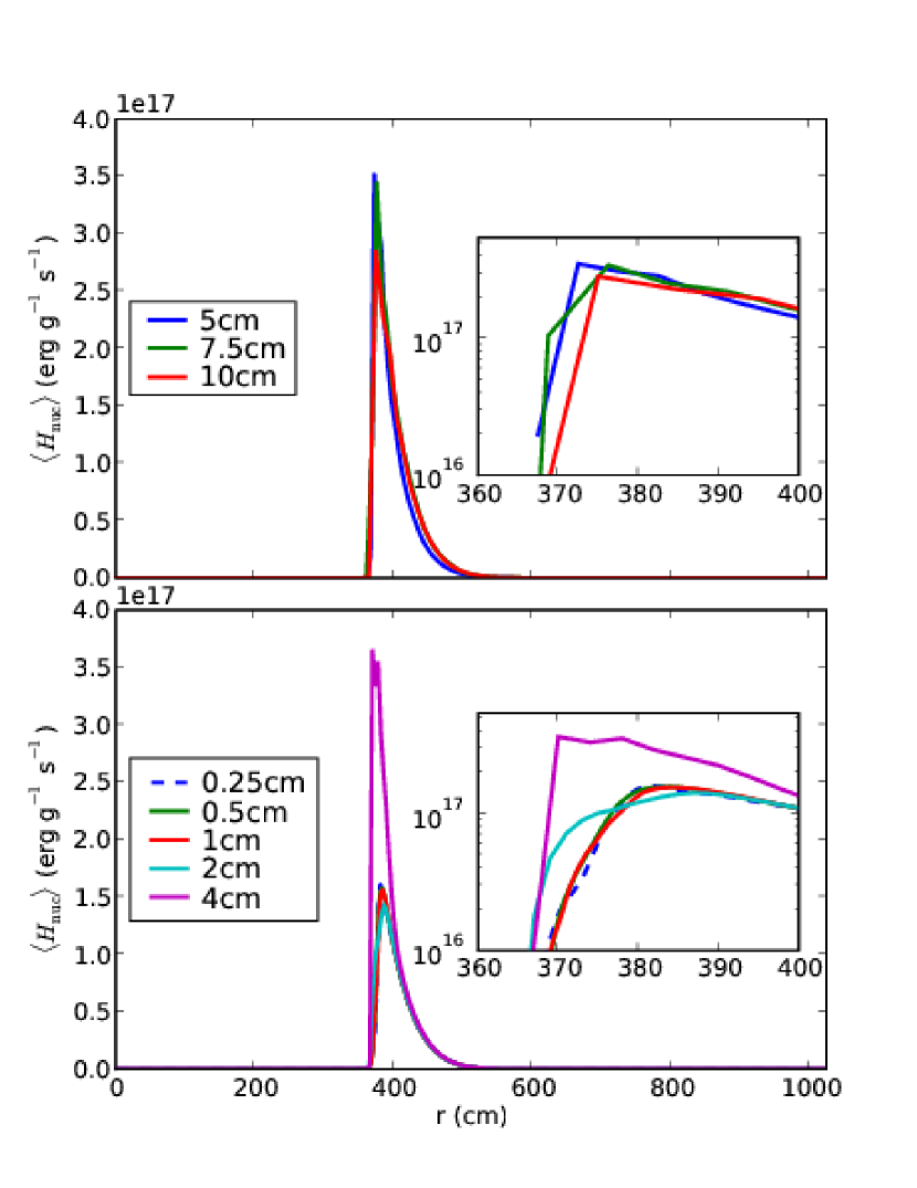
The burning layer at the base of the accreted material is very thin; high resolution is required to properly model this region. The peak of the thermal profile for the hot model is broader than the corresponding peak in the cold model. Consequently, the burning layer in the hot model is thicker than that of the cold model—we therefore focus our study of resolution requirements on the more restrictive of the two, the cold model. The top panel of Figure 3 shows the $\langle H_{\rm nuc}\rangle$ profile at $t=1$ ms for simulations of the cold model using the same resolutions as in the Lin et al. (2006) study. Even at this early time there is a $25$% spread in the peak value of $\langle H_{\rm nuc}\rangle$ for these resolutions. The bottom panel shows the same profile but at several higher resolutions. The peak value of $\langle H_{\rm nuc}\rangle$ for the $4$ cm zone^-1 simulation is comparable to the peak values in the top panel, but we only see numerical convergence of the peak value as we go to higher spatial resolution. In addition, the shape of the profile near peak converges with increasing resolution; the $0.25$ and $0.5$ cm zone^-1 resolution simulations look qualitatively similar. We therefore claim that the burning layer is not properly resolved in our models unless a resolution of $0.5$ cm zone^-1 is used. It is important to note that even though our initial models differ, this resolution requirement is an order of magnitude higher than what has been previously presented in the literature and therefore significantly increases the computational cost of our XRB simulations.

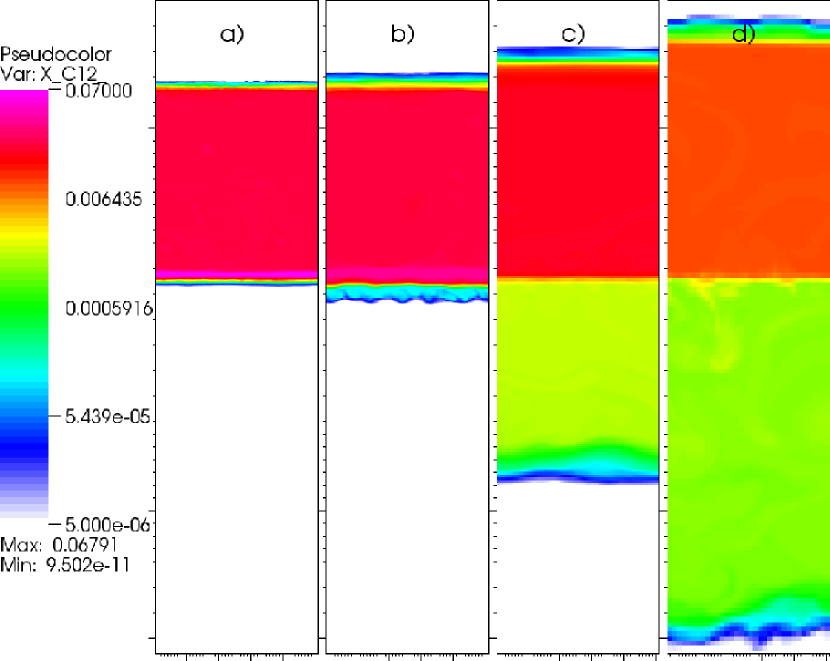
Under-resolving the burning layer artificially boosts the energy generation rate, which in turn over-drives convection. Figure 4 shows a close-up of the ¹²C mass fraction after $10$ ms of evolution of the cold model at $0.5$ (a), $2$ (b), $4$ (c), and $7.5$ cm zone^-1 (d) resolutions. The base of the burning layer is located in the bottom-most green region (just below the magenta) in panel a. All four simulations give a well-mixed carbon region above the burning layer; the extent of the convective zone increases with decreasing resolution with the $7.5$ cm zone^-1 simulation’s convective zone extending $30\%$ further than the $0.5$ cm zone^-1 simulation’s convective zone. The amount of convective undershoot—the tendency of material to penetrate below the burning layer—is much more sensitive to resolution. The $0.5$ cm zone^-1 simulation shows very little evidence of undershooting while the $7.5$ cm zone^-1 simulation has an undershoot region that is larger in physical extent than its corresponding convective region above the burning layer. For all of the studies described below, we use a resolution of $0.5$ cm zone^-1 in the burning layer.

4.2 Effects of Thermal Diffusion on the Burning Layer

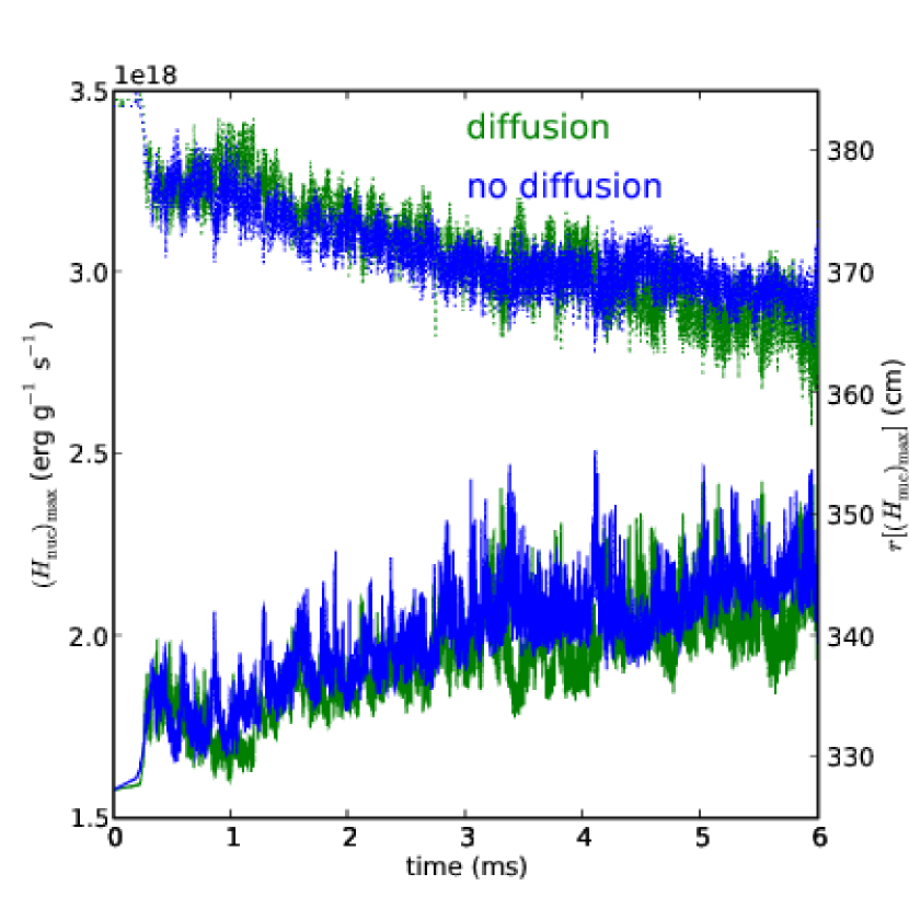
As explained in Section 1, the burning front during an XRB likely propagates as a subsonic flame, the speed of which is regulated by the rate of thermal diffusion across the front. At the resolution required to resolve the thin burning layer (see previous section) it is currently intractable to evolve the system until flame ignition. We can, however, investigate the effects of thermal diffusion on the stable burning that occurs in the burning layer. Here we focus on the hot model instead of the cold model because it has the larger thermal gradient—and hence diffusive heat flux—at the base of the accreted layer. For this simulation, we use the new adaptive mesh refinement (AMR) capability in MAESTRO (Nonaka et al., 2010), using 2 levels of refinement and ensuring that the entire convective region is at the finest level of refinement with resolution $0.5$ cm zone^-1. Figure 5 shows these effects in $\left(H_{\rm nuc}\right)_{\rm max}$ (solid lines) and the location of this maximum (dashed lines) as a function of time at early times both with (green) and without (blue) thermal diffusion. We note that the location of $\left(H_{\rm nuc}\right)_{\rm max}$ is always at the finest level of refinement. The $\left(H_{\rm nuc}\right)_{\rm max}$ evolution is similar for both cases with the magnitude in general being slightly larger for the case of no diffusion. The initial spike in $\left(H_{\rm nuc}\right)_{\rm max}$ at $t\approx 0.25$ ms is due to the fact that, initially, there is no established fluid flow that can advect away the energy released from nuclear reactions (see the discussion in Section 4.5). Over the next $3$ ms, the location of $\left(H_{\rm nuc}\right)_{\rm max}$ for both simulations moves radially inward at a rate of $\sim 2.9\times 10^{3}$ cm s^-1. Around $t=3.25$ ms, the inward radial progression of the location of $\left(H_{\rm nuc}\right)_{\rm max}$ for the simulation with no diffusion significantly slows to $\sim 900$ cm s^-1. For the remainder of the simulation, the case with thermal diffusion shows no such slowdown—heat transported radially inward via diffusion expands the lower boundary of the convective zone, which mixes fresh fuel to slightly deeper layers. By the end of the simulations, the case that included diffusion had an $\left(H_{\rm nuc}\right)_{\rm max}$ that occurred $\sim 4$ cm deeper within the atmosphere than in the case without diffusion. It should be noted that the typical standard deviation in the location of $\left(H_{\rm nuc}\right)_{\rm max}$ for the case without diffusion is of order $2$ cm; this suggests that perhaps thermal diffusion plays a role in regulating the location of maximum nuclear burning, but further evolution is needed to make statistically significant claims.

4.3 Expansion of Base State due to Heating

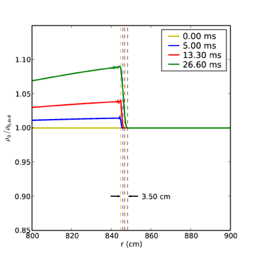
Having a dynamical base state allows us to capture the large-scale expansion of the atmosphere due to heating from nuclear reactions. This differs from the work by Lin et al. (2006), which had a time-independent base state and did not model the top of the accreted atmosphere due to numerical complications with their algorithm. Figure 6 shows the ratio of the base state density to that of the initial ($t=0$) base state density profile near the surface of the atmosphere for the cold model. We define the surface to be where $\rho_{0}=\rho_{\rm cutoff}$. The vertical dashed lines represent the location of the surface for each time-value. After $26.6$ ms of evolution, the base state has responded to heating from nuclear reactions approximately $4.5$ m below the surface by expanding $3.5$ cm. The lower Mach number flow in the cold model compared to the hot model allows for longer-term evolution of the system and therefore larger expansion of the atmosphere.

The extent of the expansion is rather small at these early times. However, as the system progresses towards outburst the energy generation and, therefore, the rate of expansion increases. As the system expands, the $p_{0}$ profile changes, which can affect the dynamics in the convective region. Additionally, as the atmosphere expands, the burning layer becomes less degenerate, which may be important for the nucleosynthesis during the outburst. Furthermore, a proper modeling of this expansion during the peak of a PRE burst model may help pinpoint the location of the photosphere with respect to the stellar radius at touchdown, a quantity that plays an important role in using XRBs to measure the mass and radius of the underlying neutron star (Steiner et al., 2010, for example).

4.4 Effects of the Volume Discrepancy Term

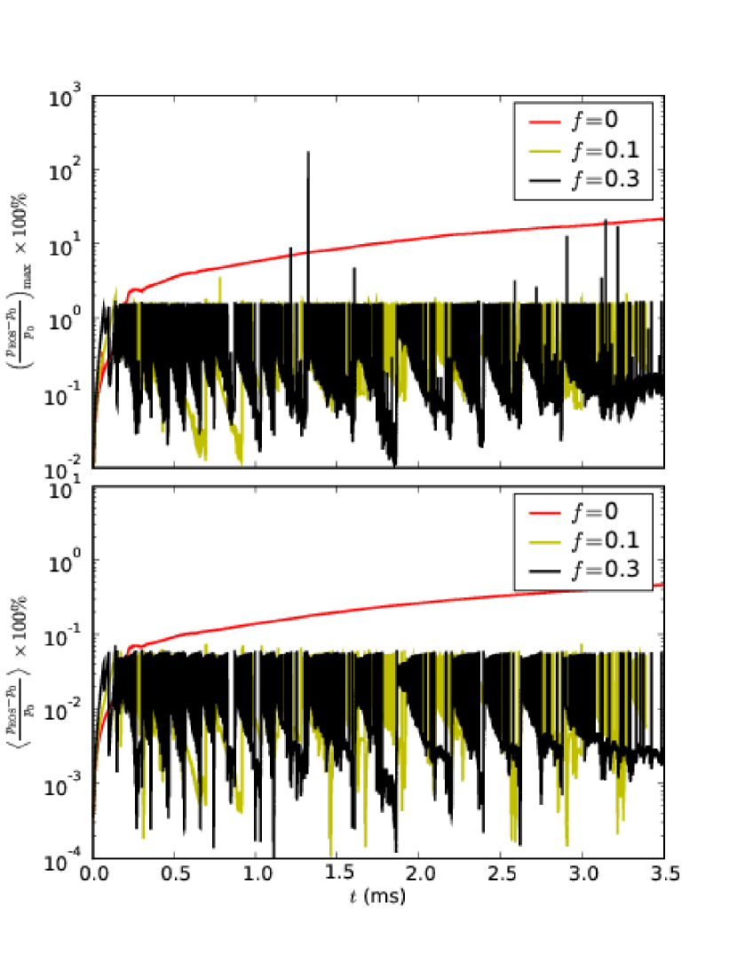
In Section 3.1 we explained that the thermodynamic pressure may drift from the base state pressure. To correct for this drift, we introduced the volume discrepancy term in equation (13), which drives the thermodynamic pressure towards the base state pressure. We focus our attention here on the hot model because it shows a more dramatic drift of the thermodynamic pressure from the base state pressure. Figure 7 shows the volume discrepancy term in action by examining the percent difference between the base state and thermodynamic pressures as a function of time for various values of $f$ for the hot model. The top panel shows the maximum value whereas the bottom panel shows the average value of this percent difference; both the peak and average values show the same trend for a given value of $f$. After the initial adjustment of the system, the average drift for the case of no volume discrepancy correction ($f=0$) increases approximately linearly at $\sim 0.1\%$ per ms of evolution. Including the correction term restricts the temporal- and spatial-averaged value of the drift to $\lesssim 0.02\%$.

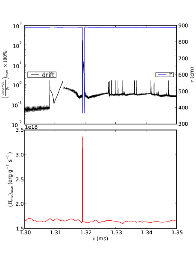
For nonzero $f$, the oscillatory behavior in the drift is due to the fact that the system may slightly over-correct the thermodynamic pressure in a given time step and then recover in the next step. A larger value of $f$ causes a stronger driving of the drift, which tends to be more oscillatory. In addition, a larger value of $f$ appears to be correlated with larger spikes in the drift. The top panel of Figure 8 shows a closeup of the $\mathcal{O}(1)$ error seen in the $f=0.3$ curve in Figure 7. The location of the maximum drift is also plotted in the top panel; the large spike in the drift occurs just below the burning layer at $r=366.25$ cm. The bottom panel of Figure 8 shows the corresponding maximum energy generation rate, which also contains a spike that is coincident with the spike in the drift—a large deposit of energy on a short timescale causes the thermodynamic pressure to get out of sync with the hydrostatic base state pressure. The increase in the energy generation rate is due to a fluid parcel rich in ⁴He fuel being brought into a region of high temperature via the turbulent convection. The duration of this transient behaviour is very short: $9$ time steps or $\sim 6.4\times 10^{-7}$ s. The selection of an appropriate non-zero value for $f$ is a problem-specific endeavor, but the chosen value has little effect on the dynamics of the convective flow field. For the simulations presented below we use a volume discrepancy correction value of $f=0.3$, which is based on the results of several test runs and past experience with comparing the results to the $f=0$ case. We will continue to study if and how the chosen value of $f$ affects the long term development of the convective field for this specific problem.

4.5 Convective Dynamics

The adiabatic excess, $\Delta\nabla$,—with

$$\Delta\nabla=\nabla-\nabla_{s},$$ (19)

where the actual thermal gradient is

$$\nabla=\frac{\partial\ln T/\partial r}{\partial\ln p/\partial r}$$

and the adiabatic thermal gradient is $\nabla_{s}=\left(d\ln T/d\ln p\right)_{s}$ with the subscript $s$ meaning along an adiabat—is used to gauge the evolution of the convective zone for the Schwarzschild instability criterion. Under this criterion, a fluid element is unstable to thermally driven convection when $\Delta\nabla>0$ and is stable for $\Delta\nabla<0$. The first term in (19) is calculated using finite differences of the temperature and pressure profiles along the radial direction. The second term in (19) depends solely on the thermodynamics of the equation of state. It is related to the second adiabatic exponent, $\Gamma_{2}$ (see Cox & Giuli (1968) Chapter 9):

$$\frac{\Gamma_{2}-1}{\Gamma_{2}}=\left(\frac{d\ln T}{d\ln p}\right)_{s}.$$ (20)

All three of the adiabatic exponents are related:

$$\frac{\Gamma_{1}}{\Gamma_{3}-1}=\frac{\Gamma_{2}}{\Gamma_{2}-1},$$ (21)

where $\Gamma_{3}-1=\left(d\ln T/d\ln\rho\right)_{\text{s}}$ and $\Gamma_{1}$ was defined in Section 3.1. Writing the equation of state as $p=p(\rho,T)$ and expanding the differential $dp$, we find the relation

$$\Gamma_{3}-1=\frac{\Gamma_{1}-\rho p_{\rho}/p}{Tp_{T}/p}$$ (22)

along an adiabat. Our equation of state only returns $\Gamma_{1}$, but combining this with (21) and (22) allows us to solve for the adiabatic thermal gradient and hence the adiabatic excess.

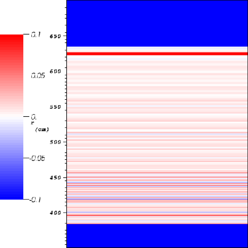
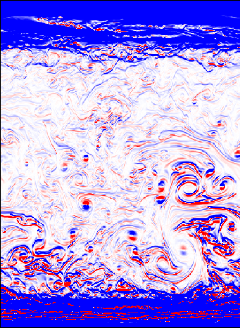
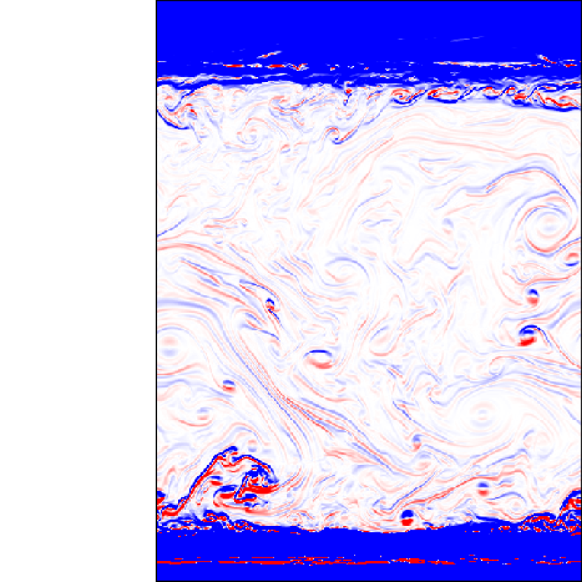
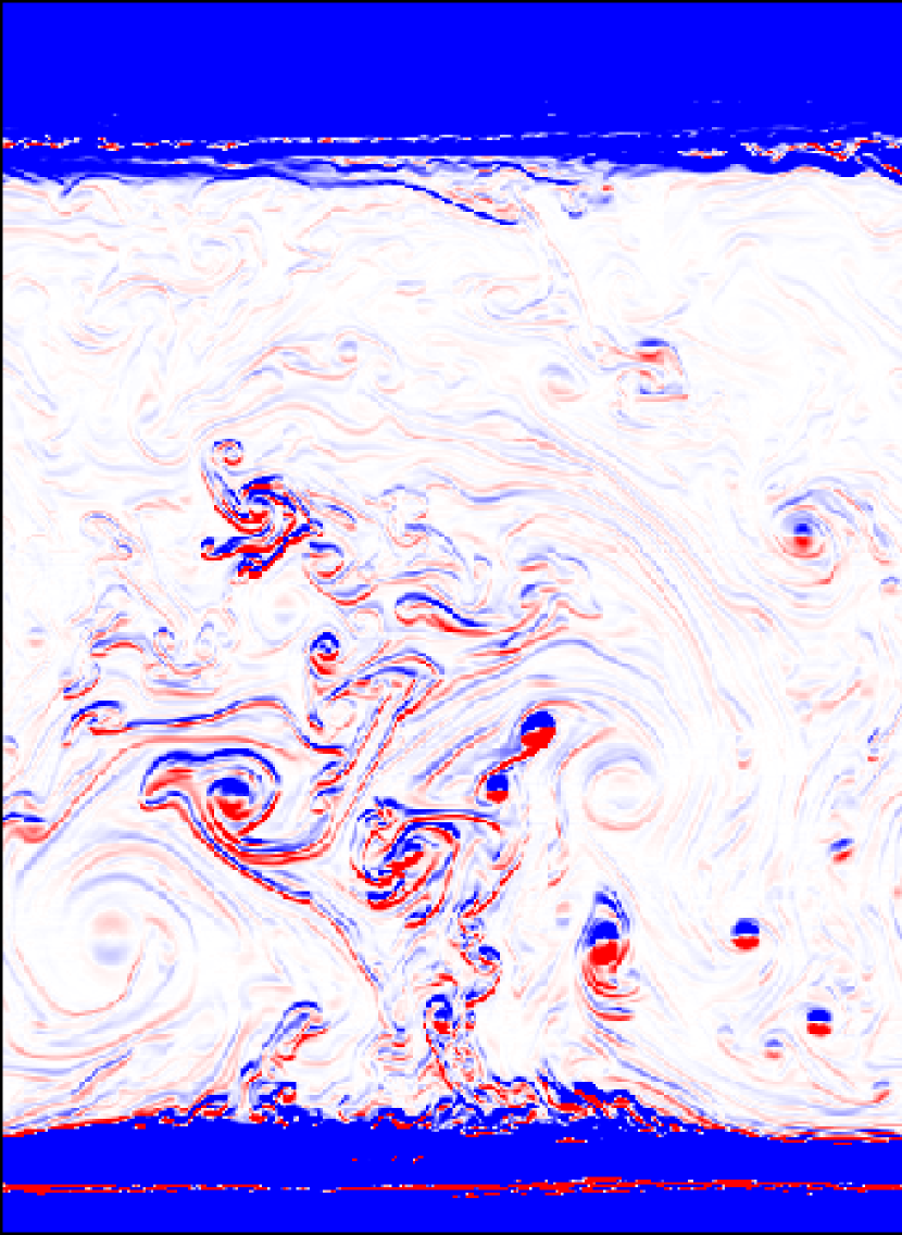
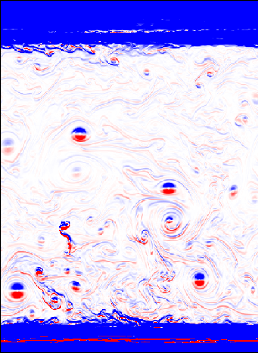
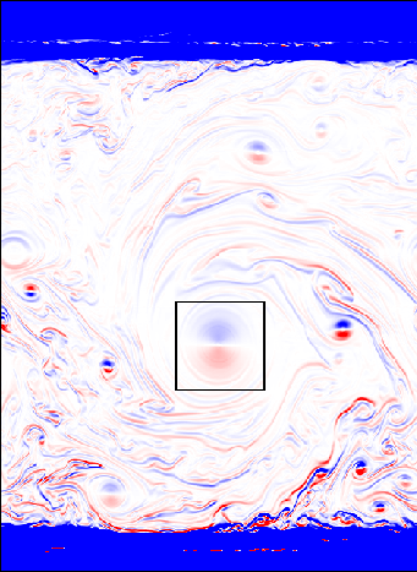
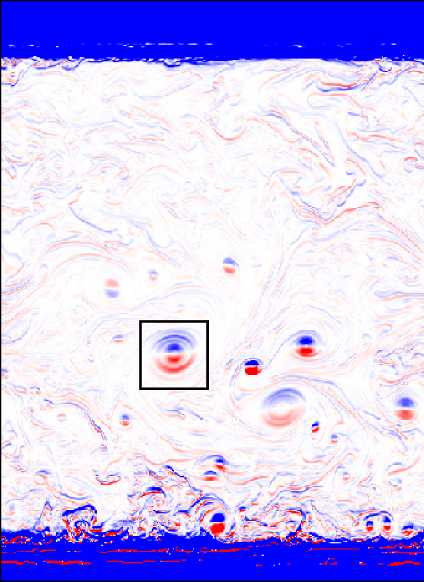
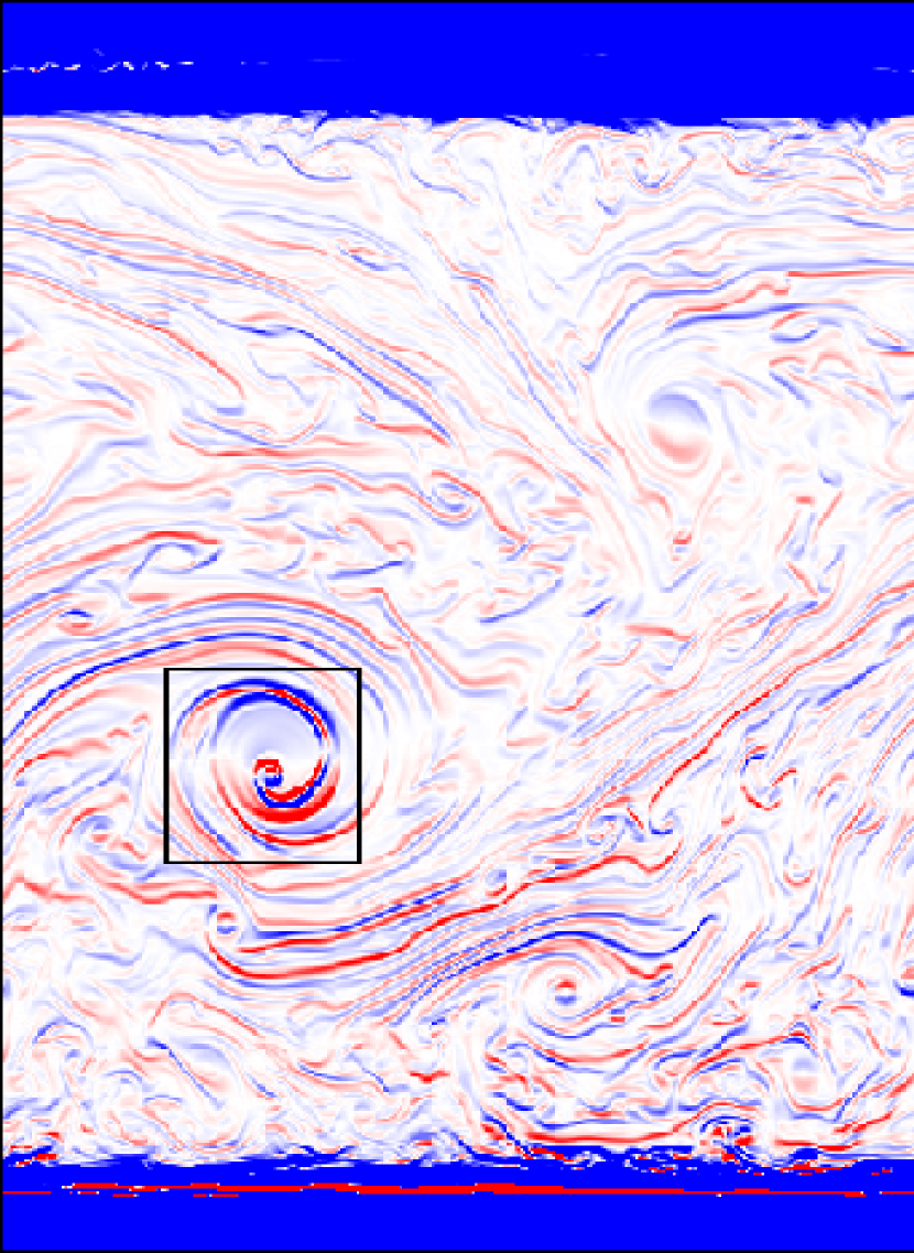
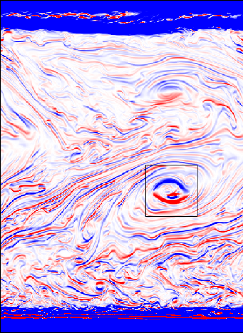
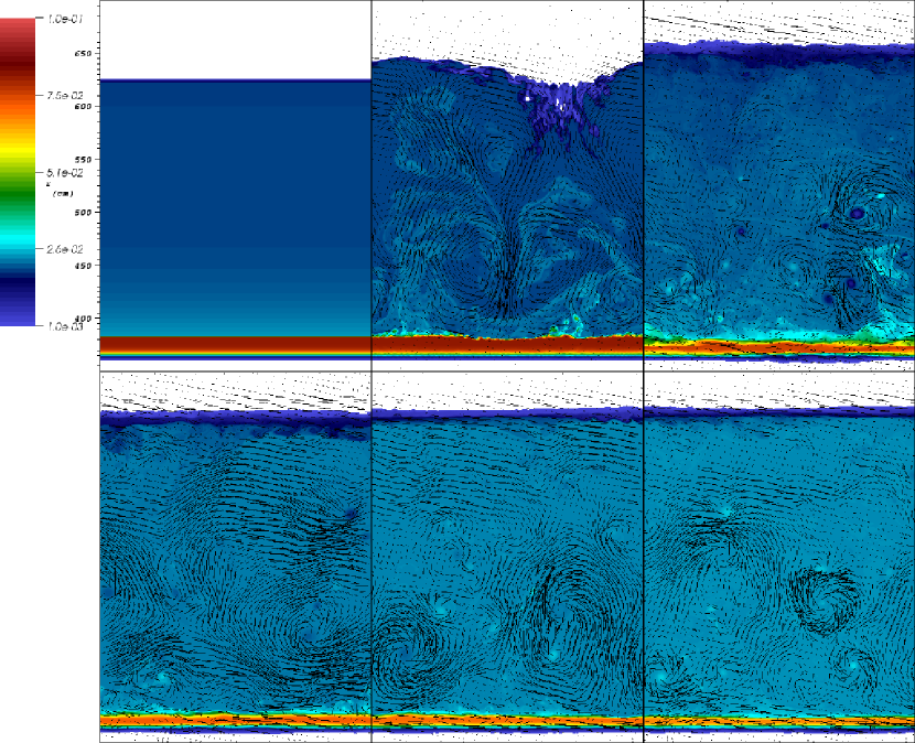
Figure 9 shows the early evolution of $\Delta\nabla$ for the cold model. Each plot covers the spatial range $(0\leq x\leq 256$ cm$,350$ cm $\leq r\leq 700$ cm$)$ to focus on the convective region. The stripes in the initial conditions, Figure 9(a), are due to small interpolation errors from mapping the initial data onto the two-dimensional grid. The initial adjustment of the system seen in Figure 9(b) causes a mixing of stable (blue) and unstable (red) fluid elements. This transient adjustment phase occurs for two reasons: 1) the initial conditions were based on a parameterization of convection in one dimension and the system now needs to adjust to a two-dimensional convective zone, and 2) the initial perturbation does not have an established convection zone and the system needs a short amount of time to build up a flow pattern associated with the perturbation. This results in mixing that produces a region that is marginally convective ($\Delta\nabla\sim 0$; white) with localized pockets of stable and unstable fluid elements as seen in Figure 9(c). At later times, these pockets further localize into vortices whose circulation gives rise to roughly circular regions of nonzero adiabatic excess—with one hemisphere that is stable and the other which is unstable—that are advected with the flow before dispersing into the ambient medium on subconvective timescales, $\sim 10^{-4}$ s. The vortices are always associated with an adiabatic excess pattern that has an unstable (red) bottom and a stable (blue) top unless two vortices are merging and interacting, in which case the stability distribution becomes skewed.

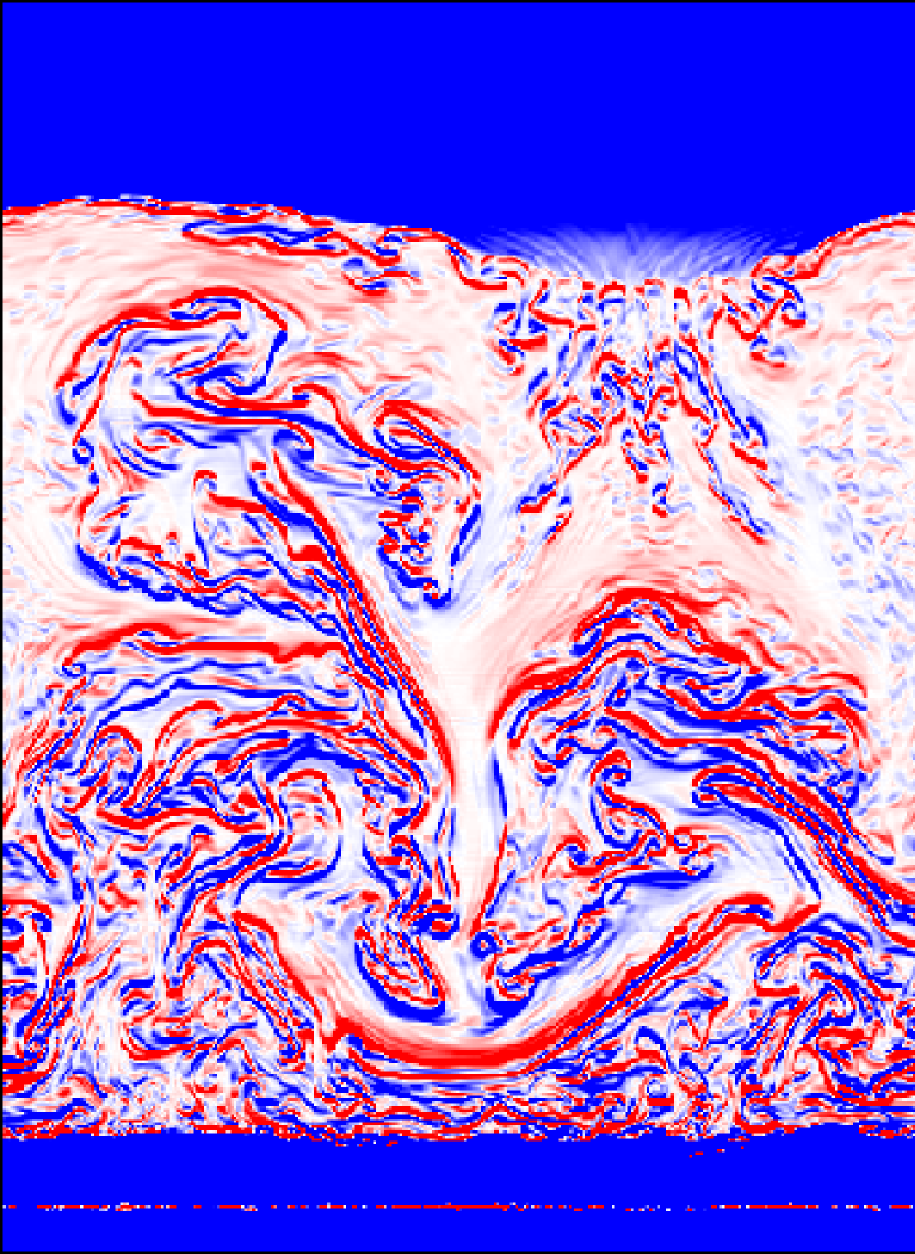
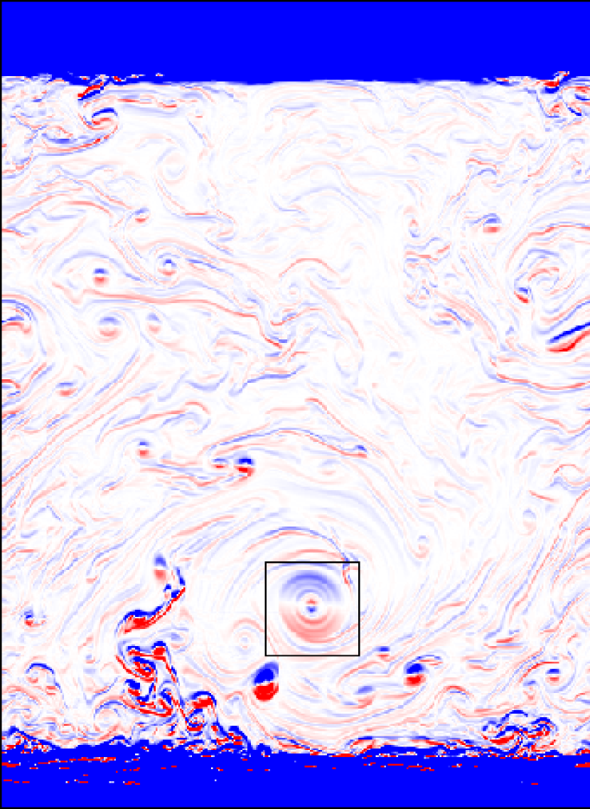
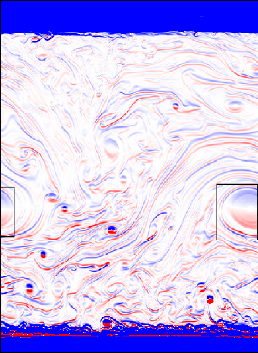
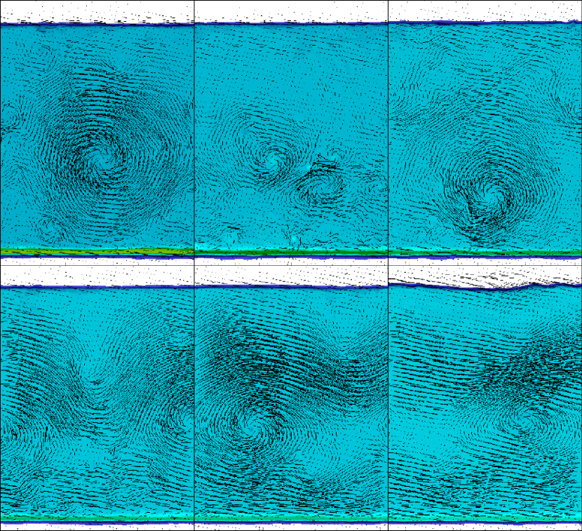
Figure 10 shows $\Delta\nabla$ for the same simulation as in Figure 9 but at later times. The boxes in these plots outline a single long-lived vortex that forms around $t=18.5$ ms, Figure 10(a), and lasts throughout the remainder of the simulation. Formation of this vortex is correlated with the formation of stronger filamentary structures, which are most clear in Figures 10(d), 10(e) and 10(f). These filaments appear to wrap around the solitary vortex and restrict the main formation of smaller vortices to the lower boundary of the convective region.

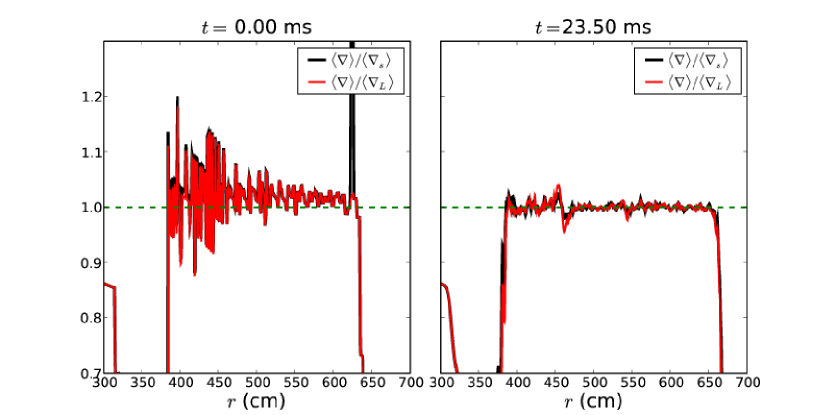
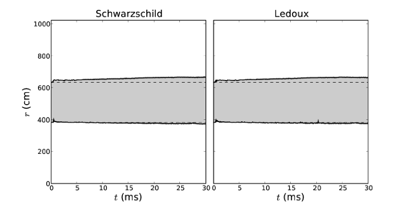
Another way to quantify the convective region is to look at the ratio $\nabla/\nabla_{s}$. From (19) we see that the system is unstable to convection under the Schwarzschild criterion when $\nabla/\nabla_{s}>1$. The Schwarzschild criterion, however, does not consider the effects of composition gradients that may help stabilize the material against convection; for this we need to consider the Ledoux criterion for instability

$$\nabla-\nabla_{L}>0,$$ (23)

where the Ledoux thermal gradient is (see, for example, Kippenhahn & Weigert (1994))

$$\nabla_{L}=\nabla_{s}-\sum_{i}\frac{\partial\ln X_{i}/\partial r}{\partial\ln p/\partial r}$$

and the second term above is evaluated via finite differences of the composition and pressure profiles. As with the Schwarzschild criterion, one can look at the ratio $\nabla/\nabla_{L}$, which is greater than unity if the material is unstable to Ledoux convection. Figure 11(a) shows the above ratios for the average thermal gradients for the initial configuration (left) and after the system has evolved for $t=23.5$ ms (right); the black line is for the case of Schwarzschild criterion convection, while the red line is for Ledoux convection. The dashed horizontal line marks the boundary for stability against convection. Where the curves lie above this line, the configuration is unstable; when convection is efficient, the curves should lie very near the horizontal line. For both the initial condition and at late times, the Schwarzschild curve and the Ledoux curve are well matched except near the edges of the convective region where composition gradients cause the two curves to deviate slightly. This is most noticeable in the initial configuration at the upper boundary where there is a sharp jump in composition, which was not smoothed (see Figure 1). Of interest in the plot at $t=23.5$ ms is the feature at $r=450$ cm, which has an unstable bottom and a stable top; this is consistent with the vortices in Figures 9 and 10, which had red bottoms and blue tops. We define the edge of the convective region to be where $\nabla/\nabla_{s}$, $\nabla/\nabla_{L}=0.75$. This particular value of $0.75$ was chosen to be sufficiently small enough to rule out false positives from strong pockets of stability from, for example, vortices within the convective region, but also large enough to rule out any fluctuations at the boundaries due to overshoot. Figure 11(b) shows in grey the extent of the convective region as a function of time with respect to the full domain for both the Schwarzschild (left) and Ledoux (right) instability criteria. The horizontal dashed lines mark the initial location of the lower and upper boundaries. The overall expansion of the upper boundary for the Schwarzschild (Ledoux) criterion is $32.0$ ($29.5$) cm in $30$ ms of evolution; the lower boundary expands downward by $9.5$ ($6.0$) cm in the same time. At late times, the upper boundary of the convective region has a much smoother composition transition than the lower boundary, therefore, the Schwarzschild and Ledoux criteria are much better matched at the upper boundary than the lower. Nevertheless, both the Ledoux and Schwarzschild criteria yield similar results when used to determine the extent of the convective region. In terms of column-depth, the convective zone after $30$ ms of evolution spans the region $2.2\times 10^{7}$ g cm${}^{-2}\lesssim y\lesssim 2.6\times 10^{8}$ g cm^-2 for both instability criteria.

For comparison, Figures 12 and 13 show the ¹²C mass fraction with velocity vectors for the same simulation and at the same times as in Figures 9 and 10, respectively. These figures clearly show the association of vortices with the circular regions of nonzero adiabatic excess seen in Figures 9 and 10. The initial adjustment of the system causes mixing that smooths the slight over-abundance of ¹²C at the base of the accreted layer present in the initial model (see Figure 1). At late times, the convective region is very well-mixed, and the ¹²C mass fraction is nearly laterally homogeneous. Furthermore, the circulation pattern associated with the long-lived vortex outlined in Figure 10 has grown to a large fraction of the convective zone and is self-interacting because of the periodic boundary conditions. The tendency of the system to form a single dominant vortex from smaller vortices is a feature of two-dimensional simulations. In three dimensions, the turbulent energy cascade moves from large to small scales; large vortical structures break down into smaller structures that are eventually dissipated by viscous effects. In two dimensions, as is the case here, the turbulent energy cascade is reversed—small vortical structures merge together to form a single dominant vortex.

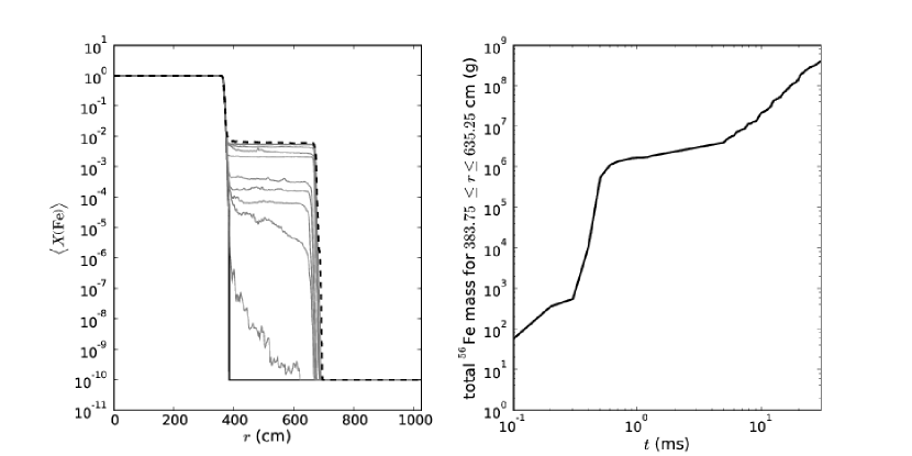
The circulation is counter-clockwise for the large, long-lived vortex; this causes a region with positive $x$-velocity below and a region of negative $x$-velocity above the vortex center. The positive $x$-velocity region extends all the way to the lower convective boundary where it causes shearing of the ⁴He/¹²C-rich region with the underlying ⁵⁶Fe region. Consequently, Figure 14 shows that some of the underlying ⁵⁶Fe neutron star material is churned up into the convective region where it is mixed with the rest of the convective material. The left panel shows average ⁵⁶Fe mass fraction profiles starting with the initial model abundance (thick solid line) through $t=30$ ms (thick dashed line); the intermediate thin solid lines show profiles at the times used in Figures 9 and 10. By $t=5$ ms, the ⁵⁶Fe is fairly well-mixed in the convective region. The right panel shows the total mass of ⁵⁶Fe in the region defined by the initial convective zone. The greatest growth in the total mass occurs, as expected, in the initial adjustment ($t\lesssim 0.6$ ms) and then flattens until large enough structures form such that there is sufficient shearing occurring at the base of the convective boundary. There is only a slight increase in the growth rate for the ⁵⁶Fe mass around $t=18.5$ ms where the long-lived vortex first appears. This is due to the fact, mentioned above, that as the system evolves it goes from many small vortices to a few large, dominant vortices. It is only when the circulation pattern of a particular vortex is large enough to strongly interact with the lower convection boundary that we get the shearing and enrichment of the convective region; this occurs around $t\sim 5$ ms. The addition of ⁵⁶Fe to the convective region has a small but noticeable effect on the conductivity; for example, a displacement of $\sim 1\%$ ⁴He for ⁵⁶Fe near the base of the accreted layer, with all other things being constant, gives a $\sim 4\%$ decrease in conductivity. This could play an important role in adjusting the flame speed once ignited.

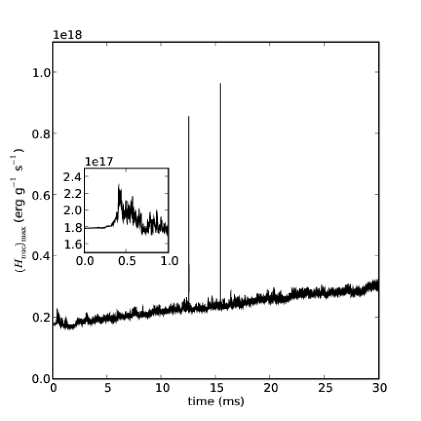
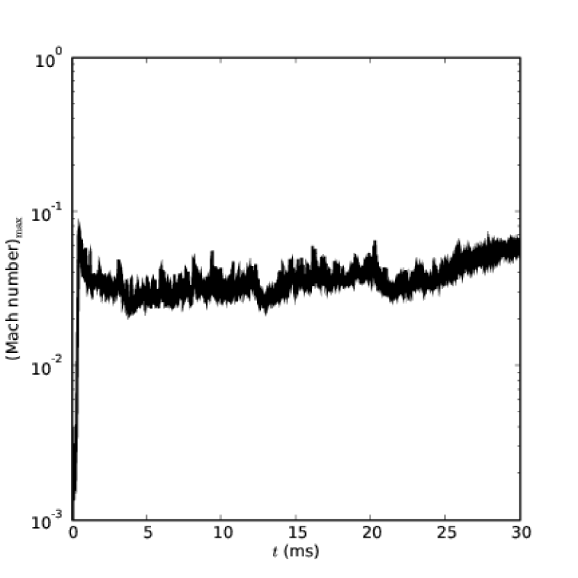
Figure 15 shows the evolution of the maximum value of $H_{\rm nuc}$ throughout the duration of the cold model simulation. The inset plot shows the early adjustment phase mentioned above. The initial jump in $H_{\rm nuc}$ is due to the fact that there is no well established flow field that can efficiently advect away the energy released from reactions. Once the convective zone is well established, the energy generation rate relaxes before making its steady climb. We note that we have not yet achieved runaway—the rise in energy generation rate is still linear. This climb is temporarily interrupted by a couple of spikes similar to those seen in Figure 8 when fresh fuel is advected to a relatively hot region and burned quickly. Although well organized at later times, the convective fluid flow is slow with respect to the sound speed. Figure 16 shows the maximum Mach number in the computational domain as a function of time; this value never exceeds $0.08$ in our simulation. The average value of the Mach number in the convective region rarely exceeds $\sim 0.02$ during our $30$ ms simulation.

5 Conclusions

We have described some of the challenges and important concepts to keep in mind when performing multidimensional simulations of XRBs. The major results can be summarized as follows:

• To get a system that is much closer to thermal instability in multiple dimensions, the semi-analytic one-dimensional models should augment the local cooling rate estimate, (4), to include cooling due to convection.

• Properly resolving the burning layer using the initial models considered here requires a spatial resolution of $0.5$ cm zone^-1, which is an order of magnitude higher than what has been presented in the literature for multidimensional models (Lin et al., 2006). It should be noted that our initial models differ in the underlying neutron star’s composition—their ¹²C opposed to our ⁵⁶Fe—and their models were evolved in one dimension through several bursts before being mapped into multiple dimensions.

• Under-resolving the burning layer leads to dramatic convective undershoot and the burning tends to die out.

• At the early times simulated here, the inclusion of thermal diffusion has little effect on the maximum energy generation rate, but does perhaps affect the depth at which this maximum occurs.

• The MAESTRO algorithm we use allows us to capture the expansion of the atmosphere due to heating, which will be important in the modeling of PRE burst sources.

• The average thermal gradient in the convective region is nearly adiabatic but there are localized pockets and filamentary structures that are either super- or sub-adiabatic.

• The strong convection interacts with and churns up the underlying neutron star material, which slightly alters the conductivity of the convective region.

The initial selection of a value to use for the volume discrepancy term in our simulations was based on experience with other applications. As we showed in Section 4.4, the value used for the long duration simulation in this paper, $f=0.3$, may not the optimal choice for the XRB problem. Further investigation is required to determine which factors affect the appropriate value of $f$, and to determine if the spikes in the drift of the thermodynamic pressure from the base state pressure are simply numerical artifacts of a poor choice of $f$.

The width of the computational domain used in our simulations is adequate for the early evolution of the system; the size of any individual convective cell is initially small with respect to the width of the domain. As the system evolves and the convection becomes more established, the cells grow in size. The nature of vorticity in two dimensions is such that the smaller vortices merge to form a single vortex. In our simulations the cells grow to become a significant fraction of the domain width and the flow becomes dominated by a single vortex that interacts with itself through the periodic boundary conditions. By selecting a wider computational grid, we could delay the formation of a single, dominant vortex. Ideally the computational domain should be several pressure scale-heights wide so that we should form multiples of these convective cells that dominate the flow for an extended period of time before merging into a single vortex. Given our strict resolution requirements, such a setup was computationally infeasible.

We plan to further investigate some of the topics mentioned above in future work while studying mixed H/He bursts. In such bursts the majority of the energy release comes from burning hydrogen; the nuclear reaction rates involved in such burning are less temperature sensitive than the $3$-$\alpha$ rate used in the current paper. This may allow for a relaxed resolution requirement for properly resolving the burning layer because the energy generation rate profile should not be as sharply peaked as we have seen in our studies. This would allow for longer time evolution, which may allow us to say something about whether or not the convective zone extends all the way to the photosphere near outburst. We will also be able to simulate larger domains where we could address the effects of domain size on the long-term evolution of the convective region and its ⁵⁶Fe enrichment. Furthermore, we will begin investigating the effects of unprecedented three-dimensional simulations of the convection that precedes the outburst in an XRB and compare its properties to our two-dimensional studies. All of these simulations will rely heavily on MAESTRO’s new AMR capability to reduce computational cost for long-term evolution. We will also investigate the effects of using different methods of calculating opacities as well as updated reaction rates, such as the $3$-$\alpha$ rate of Ogata et al. (2009).

Figure 1: Kepler-supplemented cold (solid lines) and hot (dashed lines) models as described in the text. Energy release from nuclear burning at the base of the ⁴He layer has caused the temperature to rise. The cold model is evolved to a peak $T_{\text{base}}=3.67\times 10^{8}$ K and the hot model is evolved to a peak $T_{\text{base}}=5.39\times 10^{8}$ K. The black vertical lines indicate the location of the anelastic cutoff while the grey vertical lines indicate the location of the beginning of our sponge forcing term for each of the models (see Section 3.1.)

Figure 2: Initial sponge profile for the cold model where $r_{\rm sp}=680$ cm and $r_{\rm tp}=844$ cm.

Figure 3: Average of $H_{\text{nuc}}$ as a function of height for the cold model at various resolutions at $t=1$ ms. Note that the vertical axes of the inset plots are in a logarithmic scale. For clarity, the top panel shows simulations which use the same resolutions as in the Lin et al. (2006) study and the bottom panel shows more resolved simulations. The peak of the profile at $0.5$ cm zone^-1 resolution is qualitatively similar to the peak of the profile at $0.25$ cm zone^-1 resolution.

Figure 4: Effects of under-resolving convection for the cold model. Plotted is the ¹²C mass fraction after $10$ ms of evolution for various resolutions: a) $0.5$, b) $2$, c) $4$, and d) $7.5$ cm zone^-1. Each figure shows the same region of physical space and has dimensions $256$ cm $\times$ $1024$ cm. The coarse resolution simulations show an extended convective zone and a significant amount of convective undershoot.

Figure 5: Evolution of $\left(H_{\rm nuc}\right)_{\rm max}$ (solid lines) and its vertical location (dashed lines) as a function of time for the hot model both with (green) and without (blue) thermal diffusion.

Figure 6: Expansion of the base state due to heating. Plotted is the ratio of base state density, $\rho_{0}$, to the initial ($t=0$) base state density, $\rho_{0,init}$, near the surface of the atmosphere for the cold model. We define the surface to be where $\rho=\rho_{\rm cutoff}$ and it is represented by the vertical dashed lines. The base state has expanded $3.5$ cm in $26.6$ ms of evolution.

Figure 7: Effects of the volume discrepancy factor as characterized by the percent difference between the thermodynamic pressure as given by the equation of state, $p_{\text{EOS}}$, and the base state pressure, $p_{0}$, for the hot model. The top panel shows the maximum value whereas the bottom panel shows the average value of the percent difference in the computational domain. Note the different vertical scales between the two plots.

Figure 8: Closeup of the $\mathcal{O}(1)$ spike in the maximum value of the $f=0.3$ drift as seen in the top panel of Figure 7. The top panel shows the drift value and its location in the domain; the bottom panel shows the maximum energy generation rate. The large amount of energy released from the burning spike causes the thermodynamic pressure to differ from the hydrostatic base state pressure and therefore a spike in the drift.

(a) $t=0$ ms

(b) $t=0.4$ ms

(c) $t=0.8$ ms

(d) $t=5$ ms

(e) $t=7.5$ ms

(f) $t=10$ ms

Figure 9: Colormap plot of the evolution of the adiabatic excess, $\Delta\nabla$, in the convective region for the cold model.

(a) $t=18.5$ ms

(b) $t=20.5$ ms

(c) $t=23$ ms

(d) $t=25$ ms

(e) $t=26$ ms

(f) $t=28$ ms

Figure 10: Same as Figure 9 but at later times. The boxes show the location of a single feature that, once formed, lasts for the remainder of the simulation.

(a) Example Convective Profiles

(b) Convective Region Extent

Figure 11: Analysis of the extent of the convective region. Panel (a) shows the convective profiles for both the Schwarzschild and Ledoux instability criteria at two different times. Panel (b) shows the extent of the convective region as a function of time as determined by both instability criteria.

Figure 12: Colormap plot of ¹²C mass fraction with velocity vectors for the same region and times as shown in Figure 9.

Figure 13: Colormap plot of ¹²C mass fraction with velocity vectors for the same region and times as shown in Figure 10.

Figure 14: Plots showing the ⁵⁶Fe enrichment of the convective region. The left panel shows the evolution of the average ⁵⁶Fe mass fraction starting from the initial model distribution (solid thick line) and ending after $30$ ms of evolution (dashed line); the thin grey lines show the evolution at the intermediate times shown in Figures 9 and 10. The right panel shows the total mass of ⁵⁶Fe in the convective region as a function of time. Note the log scale of the horizontal axis in the right plot.

Figure 15: Plot of the maximum $H_{\rm nuc}$ in the cold model simulation as a function of time. The inset plot shows the early adjustment phase associated with Figures 9(b) and 9(c). The spikes are similar to that seen in the bottom panel of Figure 8, and are caused by the rapid burning of fresh fuel as it is brought into the burning layer by the turbulent convection.

Figure 16: Plot of the maximum Mach number in the cold model simulation as a function of time. The slow convective flow justifies the use of a low Mach number approximation method.

Appendix A Thermal Diffusion

Here we describe the changes from Paper V due to the inclusion of the thermal conduction term in equation (9). The boldface notation refers to specific steps in the algorithm, which are fully described in Appendix A.4 in Paper V.

Applying the chain rule to the equation of state, $h=h(p_{0},T,X)$, we note that the temperature gradient can be expressed as

$$\mathbf{\nabla}T=\frac{1}{c_{p}}\mathbf{\nabla}h+\sum_{k}\frac{\xi_{k}}{c_{p}}\mathbf{\nabla}X_{k}+\frac{h_{p}}{c_{p}}\mathbf{\nabla}p_{0}.$$ (A1)

Whenever we require an explicit computation of the thermal conduction term, we use this formulation. In the edge state prediction (Steps 4H and 8H), we add an explicit contribution of the thermal conduction term to the forcing. Also, whenever we compute the expansion term $S$, we include the thermal conduction contribution. To compute thermodynamic derivatives of this term, we use $h,X$, and $p_{0}$ as inputs to the equation of state. We account for thermal diffusion in the cell update step by replacing Steps 4I and 8I with the semi-implicit approach described below.

Step 4I. Diffuse the enthalpy through a time interval of $\Delta t$.

Compute $k_{\rm th}^{(1)},c_{p}^{(1)}$, and $\xi_{k}^{(1)}$ from $\rho^{(1)},T^{(1)}$, and $X_{k}^{(1)}$ as inputs to the equation of state. We denote the result for enthalpy in Step 4H of Paper V as $(\rho h)^{(2^{\prime}),*}$ rather than $(\rho h)^{(2),*}$ to indicate that we are about to account for thermal diffusion and define $\rho^{(2^{\prime}),\star}=\rho^{(2),\star}$. The update is given by

$$(\rho h)^{(2),\star} = (\rho h)^{(2^{\prime}),\star}+\frac{\Delta t}{2}\mathbf{\nabla}\cdot\left(\frac{k_{\rm th}^{(1)}}{c_{p}^{(1)}}\mathbf{\nabla}h^{(2),\star}+\frac{k_{\rm th}^{(1)}}{c_{p}^{(1)}}\mathbf{\nabla}h^{(1)}\right)$$ (A2)

$$-\frac{\Delta t}{2}\sum_{k}\mathbf{\nabla}\cdot\left(\frac{\xi_{k}^{(1)}k_{\rm th}^{(1)}}{c_{p}^{(1)}}\mathbf{\nabla}X_{k}^{(2),\star}+\frac{\xi_{k}^{(1)}k_{\rm th}^{(1)}}{c_{p}^{(1)}}\mathbf{\nabla}X_{k}^{(1)}\right)$$

$$-\frac{\Delta t}{2}\mathbf{\nabla}\cdot\left(\frac{h_{p}^{(1)}k_{\rm th}^{(1)}}{c_{p}^{(1)}}\mathbf{\nabla}p_{0}^{(2),\star}+\frac{h_{p}^{(1)}k_{\rm th}^{(1)}}{c_{p}^{(1)}}\mathbf{\nabla}p_{0}^{(1)}\right),$$

which is numerically implemented as a diffusion equation for $h^{(2),\star}$,

$$\left(\rho^{(2),\star}-\frac{\Delta t}{2}\mathbf{\nabla}\cdot\frac{k_{\rm th}^{(1)}}{c_{p}^{(1)}}\mathbf{\nabla}\right)h^{(2),\star} = (\rho h)^{(2^{\prime}),\star}+\frac{\Delta t}{2}\mathbf{\nabla}\cdot\frac{k_{\rm th}^{(1)}}{c_{p}^{(1)}}\mathbf{\nabla}h^{(1)}$$ (A3)

$$-\frac{\Delta t}{2}\sum_{k}\mathbf{\nabla}\cdot\left(\frac{\xi_{k}^{(1)}k_{\rm th}^{(1)}}{c_{p}^{(1)}}\mathbf{\nabla}X_{k}^{(2),\star}+\frac{\xi_{k}^{(1)}k_{\rm th}^{(1)}}{c_{p}^{(1)}}\mathbf{\nabla}X_{k}^{(1)}\right)$$

$$-\frac{\Delta t}{2}\mathbf{\nabla}\cdot\left(\frac{h_{p}^{(1)}k_{\rm th}^{(1)}}{c_{p}^{(1)}}\mathbf{\nabla}p_{0}^{(2),\star}+\frac{h_{p}^{(1)}k_{\rm th}^{(1)}}{c_{p}^{(1)}}\mathbf{\nabla}p_{0}^{(1)}\right),$$

Then, update temperature using the equation of state: $T^{(2),\star}=T\left(\rho^{(2),\star},h^{(2),\star},X_{k}^{(2),\star}\right)$.

Step 8I. Diffuse the enthalpy through a time interval of $\Delta t$.

Compute $k_{\rm th}^{(2),\star},c_{p}^{(2),\star}$, and $\xi_{k}^{(2),\star}$, from $\rho^{(2),\star},T^{(2),\star}$, and $X_{k}^{(2),\star}$ as inputs to the equation of state. We also denote the result for enthalpy in Step 8H of Paper V as $(\rho h)^{(2^{\prime})}$ rather than $(\rho h)^{(2)}$ to indicate that we are about to account for thermal diffusion and define $\rho^{(2^{\prime})}=\rho^{(2)}$. The update is given by

$$(\rho h)^{(2)} = (\rho h)^{(2^{\prime})}+\frac{\Delta t}{2}\mathbf{\nabla}\cdot\left(\frac{k_{\rm th}^{(2),\star}}{c_{p}^{(2),\star}}\mathbf{\nabla}h^{(2)}+\frac{k_{\rm th}^{(1)}}{c_{p}^{(1)}}\mathbf{\nabla}h^{(1)}\right)$$ (A4)

$$-\frac{\Delta t}{2}\sum_{k}\mathbf{\nabla}\cdot\left(\frac{\xi_{k}^{(2),\star}k_{\rm th}^{(2),\star}}{c_{p}^{(2),\star}}\mathbf{\nabla}X_{k}^{(2)}+\frac{\xi_{k}^{(1)}k_{\rm th}^{(1)}}{c_{p}^{(1)}}\mathbf{\nabla}X_{k}^{(1)}\right)$$

$$-\frac{\Delta t}{2}\mathbf{\nabla}\cdot\left(\frac{h_{p}^{(2),\star}k_{\rm th}^{(2),\star}}{c_{p}^{(2),\star}}\mathbf{\nabla}p_{0}^{(2)}+\frac{h_{p}^{(1)}k_{\rm th}^{(1)}}{c_{p}^{(1)}}\mathbf{\nabla}p_{0}^{(1)}\right),$$

which is numerically implemented as a diffusion equation for $h^{(2)}$,

$$\left(\rho^{(2)}-\frac{\Delta t}{2}\mathbf{\nabla}\cdot\frac{k_{\rm th}^{(2),\star}}{c_{p}^{(2),\star}}\mathbf{\nabla}\right)h^{(2)} = (\rho h)^{(2^{\prime})}+\frac{\Delta t}{2}\mathbf{\nabla}\cdot\frac{k_{\rm th}^{(1)}}{c_{p}^{(1)}}\mathbf{\nabla}h^{(1)}$$ (A5)

$$-\frac{\Delta t}{2}\sum_{k}\mathbf{\nabla}\cdot\left(\frac{\xi_{k}^{(2),\star}k_{\rm th}^{(2),\star}}{c_{p}^{(2),\star}}\mathbf{\nabla}X_{k}^{(2)}+\frac{\xi_{k}^{(1)}k_{\rm th}^{(1)}}{c_{p}^{(1)}}\mathbf{\nabla}X_{k}^{(1)}\right)$$

$$-\frac{\Delta t}{2}\mathbf{\nabla}\cdot\left(\frac{h_{p}^{(2),\star}k_{\rm th}^{(2),\star}}{c_{p}^{(2),\star}}\mathbf{\nabla}p_{0}^{(2)}+\frac{h_{p}^{(1)}k_{\rm th}^{(1)}}{c_{p}^{(1)}}\mathbf{\nabla}p_{0}^{(1)}\right),$$

Then, update the temperature using the equation of state: $T^{(2)}=T\left(\rho^{(2)},h^{(2)},X_{k}^{(2)}\right)$.

A.1 Diffusion Solver Test

This problem is designed to test the accuracy of our implementation of an implicit solver for the diffusion of a two-dimensional Gaussian enthalpy pulse. That is, we are only concerned with the diffusive term in (9):

$$\frac{\partial(\rho h)}{\partial t}=\mathbf{\nabla}\cdot\left(k_{\rm th}\mathbf{\nabla}T\right).$$ (A6)

To easily compare with an analytic solution (see, for example Swesty & Myra (2009) for an analogous example for a radiation-hydrodynamics code) we assume the thermal conductivity to be constant: $k_{\rm th}=10^{7}\text{ erg K cm}^{-1}\text{ s}^{-1}$. Note that this does not fully test the predictor-corrector aspect of the method outlined in Appendix A because in this simplified problem $k_{\rm th}^{(2),\star}=k_{\rm th}^{(1)}$. We also assume an ideal gas with $X(\text{He}^{4})=0.5,X(\text{C}^{12})=X(\text{Fe}^{56})=0.25$ and ratio of specific heats $\gamma=5/3$. Furthermore, we are not concerned with any hydrodynamic motions so we keep the density fixed. We can then express (A6) in a simpler form:

$$\frac{\partial h}{\partial t}=D\mathbf{\nabla}^{2}h,$$ (A7)

where $D=k_{\rm th}/\left(\rho c_{p}\right)$ is the diffusion coefficient.

Given the initial conditions for the two-dimensional pulse,

$$h(\mathbf{r},t=t_{0})=(h_{\text{p}}-h_{0})\times\exp\left(\frac{-\left|\mathbf{r}-\mathbf{r_{0}}\right|^{2}}{4Dt_{0}}\right)+h_{0},$$ (A8)

where $h_{p}$, $h_{0}$, $\mathbf{r_{0}}=(x_{0},y_{0})$, and $t_{0}$ are the peak enthalpy, ambient enthalpy, location of the center of the peak, and time from which the system has evolved respectively, the analytic solution takes on the form

$$h(\mathbf{r},t)=\left(h_{\text{p}}-h_{0}\right)\left(\frac{t_{0}}{t+t_{0}}\right)\exp\left(\frac{-\left|\mathbf{r}-\mathbf{r_{0}}\right|^{2}}{4D\left(t+t_{0}\right)}\right)+h_{0},$$ (A9)

where $t$ is the evolved time.

We solve this problem on a Cartesian grid of size $4$ cm $\times$ $4$ cm with the following parameters: $h_{\text{p}}=10.0\text{ erg g}^{-1}$, $h_{0}=1.0\text{ erg g}^{-1}$, $\mathbf{r_{0}}=\left(2.0\text{ cm},2.0\text{ cm}\right)$, $t_{0}=0.1\text{ s}$, and $\rho=1.0\text{ g cm}^{-3}$. For the density and composition used in this test, we obtain a diffusion coefficient of $D=0.32\text{ cm}^{2}\text{ s}^{-1}$. As motivated in Appendix A, our implicit solve uses a Crank-Nicholson scheme that is second order accurate in space and time.

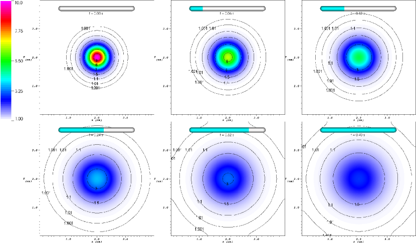
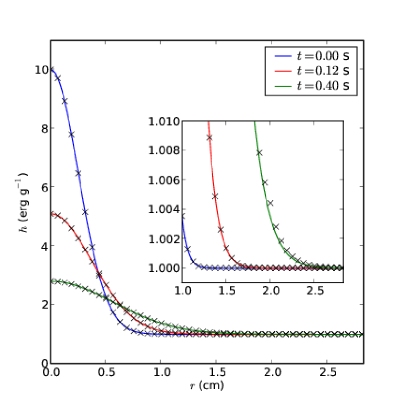
Figure 17 shows an example of the initial enthalpy pulse and its evolution through $t=0.4$ s on a $1024\times 1024$ grid with fixed time step $\Delta t=10^{-3}$ s. Note that as the pulse expands it begins to interact with the edges of the computational domain and the symmetry of the Gaussian peak is broken. Figure 18 shows the computed average enthalpy as a function of radius (X’s) compared to the analytic solution (lines) for the same test problem shown in Figure 17. Again, excepting boundary effects the numerical and analytic solutions are well matched.

To check the convergence of the algorithm we ran simulations with various resolutions and compared the errors. To measure the error in the simulation, we use the $L_{1}$ norm of the difference between the analytic and numeric solutions normalized to the $L_{1}$ norm of the analytic solution, which we define as $\varepsilon$:

$$\varepsilon^{m}\equiv\frac{||h(r,t^{m})-h^{m}||_{L_{1}}}{||h(r,t^{m})||_{L_{1}}}=\frac{\sum_{i,j}\left|h(r_{i,j},t^{m})-h_{i,j}^{m}\right|}{\sum_{i,j}|h(r_{i,j},t^{m})|},$$ (A10)

where $h(r_{i,j},t^{m})$ is the analytic solution at $r_{i,j}=\left((x_{i}-x_{0})^{2}+(y_{j}-y_{0})\right)^{1/2}$ and time $t^{m}=m\Delta t$ and $h_{i,j}^{m}$ is the numeric solution at $(x_{i},y_{j})$ and time $t^{m}$. We further define the convergence rate, $\alpha$, by comparing the value of $\varepsilon$ at the current resolution to the value of $\varepsilon$ at a finer resolution simulation:

$$\alpha\equiv\log_{2}\left(\frac{\varepsilon}{\left[\varepsilon\right]_{\text{finer}}}\right).$$ (A11)

For our comparisons, we take “finer” to mean a simulation with twice the resolution; to compare the simulations at the same physical time, the finer simulation must have evolved through twice the number of time steps as the coarser simulation. If our algorithm truly is second order accurate in space and time then $\alpha$ should equal $2$. Table 1 shows the values of $\varepsilon$ and the convergence rate for various resolutions at $t=0.08$ s; for $\alpha$, the norm in the current column is compared to the norm of the finer resolution simulation in the column to its right. Our values of $\alpha$ agree very well with the expected value.

Table 1: Reduced $L_{1}$ norms and convergence rate for the diffusion test problem at $t=0.08$ s.

	$128\times 128$ Error	$256\times 256$ Error	$512\times 512$ Error	$1024\times 1024$ Error
	$\Delta t=0.008$ s	$\Delta t=0.004$ s	$\Delta t=0.002$ s	$\Delta t=0.001$ s
$\varepsilon$	$8.64\times 10^{-5}$	$2.16\times 10^{-5}$	$5.39\times 10^{-6}$	$1.35\times 10^{-6}$
$\alpha$	$2.0012$	$1.9999$	$1.9988$	—

Figure 17: Time evolution of the diffusion of a two-dimensional Gaussian pulse of enthalpy as described in the text. The value of time displayed is the evolution time, $t$. This simulation was run with a $1024\times 1024$ grid with time step size $\Delta t=0.001$ s. Excepting edge effects near the domain boundary, the numerical solution maintains its axisymmetric form about the center of the pulse at $(x,y)=(2.0,2.0)$.

Figure 18: The average of enthalpy as a function of radius from the center, $(x,y)=(2.0,2.0)$, of a two-dimensional Gaussian pulse. The X’s are data from the numerical solution at the shown times. The lines represent the analytic solutions as given by (A9). The numerical solution tracks the analytic solution very well except when the pulse has diffused enough that it begins to interact with the boundaries of the computational domain as seen in the inset plot.

References

- Alastuey & Jancovici (1978) Alastuey, A., & Jancovici, B. 1978, ApJ, 226, 1034
- Almgren et al. (2010) Almgren, A. S. et al. 2010, Astrophysical Journal, 715, 1221
- Almgren et al. (2008) Almgren, A. S., Bell, J. B., Nonaka, A., & Zingale, M. 2008, ApJ, 684, 449, paper III
- Almgren et al. (2006a) Almgren, A. S., Bell, J. B., Rendleman, C. A., & Zingale, M. 2006a, ApJ, 637, 922, paper I
- Almgren et al. (2006b) —. 2006b, ApJ, 649, 927, paper II
- Altamirano et al. (2010) Altamirano, D., Watts, A., Linares, M., Markwardt, C. B., Strohmayer, T., & Patruno, A. 2010, ArXiv e-prints
- Arnett et al. (2008) Arnett, D., Meakin, C., Starrfield, S., Timmes, F., & Young, P. 2008, in American Institute of Physics Conference Series, Vol. 1001, Evolution and Nucleosynthesis in AGB Stars, ed. R. Guandalini, S. Palmerini, & M. Busso, 287–294
- Arnett et al. (2009) Arnett, W. D., Meakin, C., & Young, P. A. 2009, ArXiv e-prints 0910.0821
- Bhattacharyya (2010) Bhattacharyya, S. 2010, ArXiv e-prints 1001.1642
- Bildsten (2000) Bildsten, L. 2000, in American Institute of Physics Conference Series, Vol. 522, American Institute of Physics Conference Series, ed. S. S. Holt & W. W. Zhang, 359–369
- Böhm-Vitense (1958) Böhm-Vitense, E. 1958, Zeitschrift fur Astrophysik, 46, 108
- Boussinesq (1903) Boussinesq, J. 1903, Theorie analytique de la chaleur, Vol. 2 (Gauthier-Villars, Paris)
- Caughlan & Fowler (1988) Caughlan, G. R., & Fowler, W. A. 1988, Atomic Data and Nuclear Data Tables, 40, 283, see also http://www.phy.ornl.gov/astrophysics/data/cf88/index.html
- Chen et al. (2005) Chen, C.-C., Durran, D. R., & Hakim, G. J. 2005, Journal of the Atmospheric Sciences, 62, 3213
- Cox & Giuli (1968) Cox, J. P., & Giuli, R. T. 1968, Principles of stellar structure, ed. Cox, J. P. & Giuli, R. T.
- Cumming (2003) Cumming, A. 2003, ApJ, 595, 1077
- Cumming & Bildsten (2000) Cumming, A., & Bildsten, L. 2000, ApJ, 544, 453
- Durran (1990) Durran, D. 1990, Meteorol. Monographs, 23, 59
- Durran & Klemp (1983) Durran, D. R., & Klemp, J. B. 1983, Monthly Weather Review, 111, 2341
- Fryxell et al. (2000) Fryxell, B. et al. 2000, ApJS, 131, 273
- Fryxell & Woosley (1982a) Fryxell, B. A., & Woosley, S. E. 1982a, ApJ, 258, 733
- Fryxell & Woosley (1982b) —. 1982b, ApJ, 261, 332
- Fushiki & Lamb (1987) Fushiki, I., & Lamb, D. Q. 1987, ApJ, 323, L55
- Graboske et al. (1973) Graboske, H. C., Dewitt, H. E., Grossman, A. S., & Cooper, M. S. 1973, ApJ, 181, 457
- Heger et al. (2007a) Heger, A., Cumming, A., Galloway, D. K., & Woosley, S. E. 2007a, ApJ, 671, L141
- Heger et al. (2007b) Heger, A., Cumming, A., & Woosley, S. E. 2007b, ApJ, 665, 1311
- Heger et al. (2000) Heger, A., Langer, N., & Woosley, S. E. 2000, ApJ, 528, 368
- Kesel & Winninghoff (1972) Kesel, P. G., & Winninghoff, F. J. 1972, Monthly Weather Review, 100, 360
- Kippenhahn & Weigert (1994) Kippenhahn, R., & Weigert, A. 1994, Stellar Structure and Evolution, ed. Kippenhahn, R. & Weigert, A.
- Lin et al. (2006) Lin, D. J., Bayliss, A., & Taam, R. E. 2006, ApJ, 653, 545
- Muno et al. (2002) Muno, M. P., Chakrabarty, D., Galloway, D. K., & Psaltis, D. 2002, ApJ, 580, 1048
- Narayan & Cooper (2007) Narayan, R., & Cooper, R. L. 2007, ApJ, 665, 628
- Nonaka et al. (2010) Nonaka, A., Almgren, A. S., Bell, J. B., Lijewski, M. J., Malone, C. M., & Zingale, M. 2010, ApJS, 188, 358, paper V
- Ogata et al. (2009) Ogata, K., Kan, M., & Kamimura, M. 2009, Progress of Theoretical Physics, 122, 1055
- Ogura & Phillips (1962) Ogura, Y., & Phillips, N. A. 1962, Journal of Atmospheric Sciences, 19, 173
- Pember et al. (1998) Pember, R. B., Howell, L. H., Bell, J. B., Colella, P., Crutchfield, C. Y., Fiveland, W. A., & Jessee, J. P. 1998, Combustion Science and Technology, 140, 123
- Perkey & Kreitzberg (1976) Perkey, D. J., & Kreitzberg, C. W. 1976, Monthly Weather Review, 104, 744
- Shara (1982) Shara, M. M. 1982, ApJ, 261, 649
- Spitkovsky et al. (2002) Spitkovsky, A., Levin, Y., & Ushomirsky, G. 2002, Astrophysical Journal, 566, 1018
- Steiner et al. (2010) Steiner, A. W., Lattimer, J. M., & Brown, E. F. 2010, ArXiv e-prints
- Strohmayer & Bildsten (2006) Strohmayer, T., & Bildsten, L. 2006, Compact Stellar X-Ray Sources, ed. W. H. G. Lewin & M. van der Klis (Cambridge: Cambridge Univ. Press), 113–+
- Strohmayer et al. (1996) Strohmayer, T. E., Zhang, W., Swank, J. H., Smale, A., Titarchuk, L., Day, C., & Lee, U. 1996, ApJ, 469, L9+
- Swesty & Myra (2009) Swesty, F. D., & Myra, E. S. 2009, ApJS, 181, 1
- Taam et al. (1993) Taam, R. E., Woosley, S. E., Weaver, T. A., & Lamb, D. Q. 1993, ApJ, 413, 324
- Timmes (2000) Timmes, F. X. 2000, ApJ, 528, 913, source code obtained from http://cococubed.asu.edu/code_pages/kap.shtml
- Timmes & Swesty (2000) Timmes, F. X., & Swesty, F. D. 2000, ApJS, 126, 501, source code obtained from http://cococubed.asu.edu/codes/eos.shtml/helmholtz.tbz
- Weaver et al. (1978) Weaver, T. A., Zimmerman, G. B., & Woosley, S. E. 1978, ApJ, 225, 1021
- Woosley & Weaver (1984) Woosley, S. E., & Weaver, T. A. 1984, in American Institute of Physics Conference Series, Vol. 115, American Institute of Physics Conference Series, ed. S. E. Woosley, 273–+
- Zingale et al. (2009) Zingale, M., Almgren, A. S., Bell, J. B., Nonaka, A., & Woosley, S. E. 2009, Astrophysical Journal, 704, 196
- Zingale et al. (2002) Zingale, M. et al. 2002, Astrophysical Journal Supplement, 143, 539
- Zingale et al. (2001) —. 2001, Astrophysical Journal Supplement, 133, 195