Do spectra improve distance measurements of Type Ia supernovae?

We investigate the use of a wide variety of spectroscopic measurements to determine distances to low-redshift Type Ia supernovae (SN Ia) in the Hubble flow observed through the CfA Supernova Program. We consider linear models for predicting distances to SN Ia using light-curve width and color parameters (determined using the SALT2 light-curve fitter) and a spectroscopic indicator, and evaluate the resulting Hubble diagram scatter using a cross-validation procedure. We confirm the ability of spectral flux ratios alone at maximum light to reduce the scatter of Hubble residuals by $\sim 10$% [weighted rms, or ${\rm WRMS}=0.189\pm 0.026$ mag for the flux ratio $\mathcal{R}(6630/4400)$] with respect to the standard combination of light-curve width and color, for which ${\rm WRMS}=0.204\pm 0.029$ mag. When used in combination with the SALT2 color parameter, the color-corrected flux ratio $\mathcal{R}^{c}(6420/5290)$ at maximum light leads to an even lower scatter (${\rm WRMS}=0.175\pm 0.025$ mag), although the improvement has low statistical significance ($<2\sigma$) given the size of our sample (26 SN Ia). We highlight the importance of an accurate relative flux calibration and the failure of this method for highly-reddened objects. Comparison with synthetic spectra from 2D delayed-detonation explosion models shows that the correlation of $\mathcal{R}(6630/4400)$ with SN Ia absolute magnitudes can be largely attributed to intrinsic color variations and not to reddening by dust in the host galaxy. We consider flux ratios at other ages, as well as the use of pairs of flux ratios, revealing the presence of small-scale intrinsic spectroscopic variations in the iron-group-dominated absorption features around $\sim 4300$ Å and $\sim 4800$ Å. The best flux ratio overall is the color-corrected $\mathcal{R}^{c}(4610/4260)$ at $t=-2.5$ d from maximum light, which leads to $\sim 30$% lower scatter (${\rm WRMS}=0.143\pm 0.020$ mag) with respect to the standard combination of light-curve width and color, at $\sim 2\sigma$ significance. We examine other spectroscopic indicators related to line-profile morphology (absorption velocity, pseudo-equivalent width etc.), but none appear to lead to a significant improvement over the standard light-curve width and color parameters. We discuss the use of spectra in measuring more precise distances to SN Ia and the implications for future surveys which seek to determine the properties of dark energy.

1 Introduction

Precise distances to Type Ia supernovae (SN Ia) formed the cornerstone of the discovery of cosmic acceleration (Riess et al. 1998; Perlmutter et al. 1999). These measurements use the shape of supernova light curves and their colors to tell which supernovae are bright and which are intrinsically dim (Phillips 1993; Riess et al. 1996; Prieto et al. 2006; Jha et al. 2007; Guy et al. 2007; Conley et al. 2008; Mandel et al. 2009). In this paper we explore the suggestion of Bailey et al. (2009) that spectra can contribute to improved distance measurements. We apply statistical tests to a subset of the $\sim 250$ SN Ia for which we have good light curves and spectra based on the ongoing program of supernova observations at the Harvard-Smithsonian Center for Astrophysics (CfA; Matheson et al. 2008; Hicken et al. 2009a).

It is important to construct the best possible distance indicators to extract the maximum cosmological information from supernova surveys. The present state-of-the-art gives distances to well-observed individual objects with uncertainties of order 10%, so that samples of nearby (Hicken et al. 2009b) and distant SN Ia (ESSENCE, Miknaitis et al. 2007; SNLS, Astier et al. 2006) can be combined to constrain the equation-of-state for dark energy, noted $w$. The first results show that for a flat universe with constant $w$, the dark energy is compatible with a cosmological constant (for which $w=-1$) within about 10% (Astier et al. 2006; Wood-Vasey et al. 2007). Constraints on the variation of $w$ with redshift come from from high-redshift observations with the Hubble Space Telescope (Riess et al. 2004, 2007). Present-day limits are weak, but future work with large, carefully calibrated samples from the ground (Pan-STARRS, Dark Energy Survey, LSST) and from space (Euclid, WFIRST) will contribute to distinguishing the nature of dark energy (Albrecht et al. 2009). In designing the follow-up observations for these enterprises, it is worth knowing whether spectra will be useful only for classification and precise redshifts, or whether the spectra of the supernovae themselves can be used to improve the precision of the distances. The way we explore this is to analyze the CfA sample, using the difference between the distance derived from Hubble expansion with the distance predicted from our various models. This difference is the Hubble residual, which we use as a measure of the power of a particular model to predict the supernova distance. As described below, we explore models that combine quantitative information from the spectrum with information on light curve shape and color.

Spectroscopic information is fundamental to the success of employing SN Ia as distance indicators in large surveys. Cleanly separating Type Ia supernovae from core-collapse events like SN Ib and SN Ic improves the purity of the sample. More directly, Nugent et al. (1995) showed that some easily-measured line ratios in SN Ia spectra are correlated with the luminosity. Measurements of line velocities (and gradients thereof), strengths, and widths and their relation to supernova luminosity have been explored recently by several authors (Benetti et al. 2005; Blondin et al. 2006; Bongard et al. 2006; Hachinger et al. 2006; Bronder et al. 2008). Likewise, Matheson et al. (2008) revealed spectroscopic variability amongst SN Ia of similar luminosity. But the first application of spectroscopic clues to improve distance estimates has come from Bailey et al. (2009). Using spectra of 58 SN Ia from the Nearby Supernova Factory, they showed that the ratio of fluxes in selected wavelength bins (flux ratios) could reduce the scatter of Hubble residuals by $\sim 20$% compared to the usual combination of light-curve width and color parameters ($\sigma=0.128\pm 0.012$ mag cf. $0.161\pm 0.015$ mag). By using a flux ratio measured on a de-reddened spectrum in combination with a color parameter they found a further $\sim 5$% improvement ($\sigma=0.119\pm 0.011$ mag). We have sought first to see if we can reproduce their results using the CfA data set, and then to test additional ideas about ways to use spectra to improve the estimates of supernova distances.

In practice, the standardization of SN Ia magnitudes involves a term related to the width of the light curve and a correction due to color. While some methods attempt to separate intrinsic color variations from reddening by dust in the host galaxy (e.g., MLCS2k2; Jha et al. 2007) others use a single parameter for both effects (e.g. SALT2; Guy et al. 2007), exploiting the degeneracy between the two: underluminous SN Ia are also intrinsically redder than overluminous SN Ia (e.g. Tripp 1998). We adopt the latter approach in this paper, to match the method used by Bailey et al. (2009). An active area of research involves the use of SN Ia spectra to provide independent or complementary information on SN Ia luminosities that would help improve their use as distance indicators.

We consider models for predicting distances to SN Ia of the form:

$$\mu=m_{B}-M+(\alpha\times{\rm width})-(\beta\times{\rm color})+(\gamma\times{\rm spec}),$$ (1)

where $m_{B}$ is the apparent rest-frame $B$-band magnitude at peak, $M$ is a reference absolute magnitude, “width” and “color” are the usual light-curve parameters, and “spec” is some spectroscopic indicator; $(\alpha,\beta,\gamma)$ are fitting constants. We study the following five models:

• only a spectroscopic indicator is used [i.e. $(\alpha,\beta)=(0,0)$],

• both a spectroscopic indicator and a light-curve width parameter are used, but no color parameter (i.e. $\beta=0$),

• both a spectroscopic indicator and a color parameter are used, but no light-curve width parameter (i.e. $\alpha=0$),

• a spectroscopic indicator is used in addition to the light-curve width and color parameters.

• both light-curve width and color parameters are used, but no spectroscopic indicator (i.e. $\gamma=0$). We refer to this as the “standard” model.

We refer to the set of light-curve parameters and spectroscopic indicators in a given model as the “predictors” for that model, as is common practice in the field of statistics. We can evaluate the use of including a spectroscopic indicator (models 1-4) by comparing the resulting scatter of Hubble diagram residuals with that from the standard model (No. 5).

The paper is organized as follows: in § 2 we present our light-curve fitting and training method, as well as a cross-validation procedure to evaluate the impact of each spectroscopic indicator. We present the CfA data set in § 3. In § 4 we study the flux ratios of Bailey et al. (2009), while in § 5 we consider other spectroscopic indicators. We discuss the use of SN Ia spectra for distance measurements in § 6 and conclude in § 7.

2 Methodology

2.1 Light-curve fitting

We use the SALT2 light-curve fitter of Guy et al. (2007) to determine the width and color parameters for each SN Ia in our sample. A model relating distance, apparent magnitudes, and linear dependencies of the absolute magnitude is:

$$\mu=m_{B}-M+\alpha x_{1}-\beta c+\gamma\mathcal{S},$$ (2)

where $(x_{1},c)$ are the SALT2 light curve width and color parameters, and $\mathcal{S}$ is some spectroscopic indicator. The rest-frame peak apparent $B$-band magnitude is $m_{B}$, also obtained from the SALT2 fit to a supernova’s light curve. The distance modulus predicted from the light curve and spectral indicators is $\mu$, and the constant $M$ is a reference absolute magnitude. The distance modulus estimated from the redshift is $\mu(z)=25+5\log_{10}[D_{L}(z)\text{Mpc}^{-1}]$ under a fixed cosmology, where $D_{L}$ is the luminosity distance.

We use the exact same SALT2 options as Guy et al. (2007) to fit the SN Ia light curves in our sample, and only trust the result when the following conditions are met: reduced $\chi^{2}_{\nu}\leq 2$; at least one $B$-band point before +5 d from $B$-band maximum, and one after +10 d; at least 5 $B$- and $V$-band points in the age range $-15\leq t\leq+60$ d; finally, we impose a cut on the SALT2 $x_{1}$ parameter, namely $-3\leq x_{1}\leq 2$. This last condition is equivalent to considering SN Ia in the range $0.8\lesssim\Delta m_{15}(B)\lesssim 1.7$ (i.e. subluminous 1991bg-like SN Ia are excluded). We examined all the light-curve fits by eye to ensure they were satisfactory given this set of conditions. Approximately 170 of the $\sim 250$ SN Ia with light curves from the CfA SN program pass these requirements.

2.2 Training

For estimating the coefficients of the model (training), we use a custom version of the luminosity distance fitter simple_cosfitter (A. Conley 2009, private communication) based on the Minuit function minimization package (James & Roos 1975). This code minimizes the following expression with respect to the parameters $(\alpha,\beta,\gamma,\mathcal{M})$:

$$\begin{split}\chi^{2}&=\sum_{s=1}^{N}\frac{[m_{B,s}-m_{{\rm pred},s}(z_{s};x_{1}^{s},c_{s},\mathcal{S}_{s};\alpha,\beta,\gamma,\mathcal{M})]^{2}}{\sigma_{s}^{2}}\\ &=\sum_{s=1}^{N}\frac{[\mu(m_{B}^{s},x_{1}^{s},c_{s},\mathcal{S}_{s};\alpha,\beta,\gamma,M)-\mu(z_{s})]^{2}}{\sigma_{s}^{2}}\end{split}$$ (3)

where $m_{B,s}$ is the rest-frame peak apparent $B$-band magnitude of the $s^{\rm th}$ SN Ia, and $m_{{\rm pred},s}$ is the predicted peak apparent $B$-band magnitude, given by:

$$m_{{\rm pred},s}=5\log_{10}D_{L}(z_{s})-\alpha x_{1,s}+\beta c_{s}-\gamma\mathcal{S}_{s}+\mathcal{M},$$ (4)

where $D_{L}$ is the luminosity distance at redshift $z_{s}$ for a given cosmological model described by the standard parameters $(w,\Omega_{m},\Omega_{\Lambda})$. Since our analysis only includes objects at low redshifts ($z<0.06$), we do not solve for these parameters and simply assume a flat, cosmological constant-dominated model with $(w,\Omega_{m},\Omega_{\Lambda})=(-1,0.27,0.73)$. The $\mathcal{M}$ term is a collection of constants including the reference $M$.

The variance $\sigma_{s}^{2}$ that appears in the denominator of Eq. 3 includes an error on the corrected magnitude (Eq. 2), using the estimation error covariance of the light-curve parameters and spectroscopic indicators, a variance due to peculiar velocities [$\sigma_{{\rm pec},s}=(v_{\rm pec}/cz_{s})(5/\ln 10)$, where we take the rms peculiar velocity $v_{\rm pec}=300$   km  s^-1], and an intrinsic dispersion of SN Ia magnitudes:

$$\sigma_{s}^{2}=\sigma_{m,s}^{2}+\sigma_{{\rm pec},s}^{2}+\sigma_{\rm int}^{2},$$ (5)

where $\sigma_{\rm int}$ is adjusted iteratively until $\chi^{2}_{\nu}\approx 1$ [typically $\sigma_{\rm int}\lesssim 0.2$ mag for the standard $(x_{1},c)$ model]. For any particular model, the intrinsic variance $\sigma_{\rm int}^{2}$ accounts for deviations in magnitude in the Hubble diagram beyond that explained by measurement error or random peculiar velocities, and hence represents a floor to how accurately the model can predict distances. To limit the impact of the peculiar velocity error we restrict our analysis to SN Ia at redshifts $z>0.015$ ($\sigma_{\rm pec}<0.15$ mag). Of the 170 SN Ia with satisfactory SALT2 fits, 114 are at redshifts greater than 0.015.

2.3 Cross-validation

We consider several models described by Eq. 2 that use different subsets of the predictors $(x_{1},c,\mathcal{S}$). If we train a model on the data of all the SN in the sample to estimate the coefficients $(\hat{\alpha},\hat{\beta},\hat{\gamma},\hat{\mathcal{M}})$, we can evaluate the fit of the model by computing the training error, e.g. the mean squared distance modulus residual, $\mu(m_{B}^{s},x_{1}^{s},c_{s},\mathcal{S}_{s};\hat{\alpha},\hat{\beta},\hat{\gamma},\hat{M})-\mu(z_{s})$, over all SN $s$ in the training set.

For finite samples, the average Hubble diagram residual of the training set SN is an optimistic estimate of the ability of the statistical model, Eq. 2, to make accurate predictions given the supernova observables. This is because it uses the supernova data twice: first for estimating the model parameters (training), and second in evaluating the residual error. Hence, the training set residuals underestimate the prediction error, which is the expected error in estimating the distance of a SN that was not originally in the finite training set. We refer to these data as “out-of-sample”. Furthermore, with a fixed, finite, and noisy training data set, it is always possible to reduce the residual, or training, error of the fit by introducing more predictors to the model. However, this may lead to over-fitting, in which apparently significant predictors are found in noisy data, even though in reality there was no trend. These relationships are sensitive to the finite training set and would not generalize to out-of-sample cases. To evaluate predictive performance and guard against over-fitting with a statistical model based on finite data, we should estimate the prediction error for out-of-sample cases. To do so, we use a cross-validation (CV) procedure to evaluate the impact of using a spectroscopic indicator $\mathcal{S}$, alone and in conjunction with standard light curve parameters, on the accuracy of distance predictions in the Hubble diagram.

Cross-validation seeks to estimate prediction error and to test the sensitivity of the trained statistical model to the data set by partitioning the full data set into smaller subsets. One subset is held out for testing predictions of the model, while its complement is used to train the model. This process is repeated over partitions of the full data set. This method avoids using the same data simultaneously for training the model and for estimating its prediction error. Cross-validation was used before for statistical modeling of SN Ia by Mandel et al. (2009), who applied the .632 bootstrap method to evaluate distance predictions for SN Ia using near infrared light curves. A careful implementation of a cross-validation method is particularly important for small samples, as is the case in this paper (e.g. 26 SN Ia at maximum light; see § 4.3).

In this paper, the cross-validation method we use is known as $K$-fold CV. The idea is to divide our SN Ia sample into $K$ subsets, train a given model on $K-1$ subsets, and validate it on the remaining subset. This procedure is repeated $K$ times, at which point all SN Ia have been part of a validation set once. Typical choices of $K$ are 5 or 10 (e.g., Hastie et al. 2009). The case $K=N$, where $N$ is the number of SN Ia in our sample, is known as “leave-one-out” CV. In this case, each SN Ia in turn is used as a validation set, and the training is repeated $N$ times on $N-1$ SN Ia.

In practice, we run $K$-fold CV as follows:

• the sample of $N$ SN Ia is randomly divided into $K$ subsets of equal size (when $N$ is not a multiple of $K$, the number of SN Ia between any two subsets differs by at most one).

• Looping over each $K$ fold:

  • all the SN Ia in the $K^{\rm th}$ subset are removed from the sample: they form the validation set. The remaining SN Ia define the training set.

  • the objects in the training set are then used to determine the best-fit values for the parameters $(\hat{\alpha}_{K},\hat{\beta}_{K},\hat{\gamma}_{K},\hat{\mathcal{M}}_{K})$ in Eq. 3, as well as the intrinsic dispersion $\sigma_{\rm int}$ in Eq. 5.

  • using this set of parameters we predict the magnitudes of the SN Ia in the validation set (indexed $j$):

    $$m_{{\rm pred},j}=5\log_{10}D_{L}(z_{j})-\alpha_{K}x_{1,j}+\beta_{K}c_{j}-\gamma_{K}\mathcal{S}_{j}+\mathcal{M}_{K}.$$ (6)

    The Hubble residual, or error, of the predicted distance modulus is then

    $$\Delta\mu_{j}=m_{B,j}-m_{{\rm pred},j}=\mu(m_{B}^{j},x_{1}^{j},c_{j},\mathcal{S}_{j};\alpha,\beta,\gamma,M)-\mu(z_{j}).$$ (7)

• When the magnitude or distance of each SN Ia has been predicted once using the above scheme, we analyze the prediction errors (§2.4). When doing so, we check that the set of best-fit $(\hat{\alpha}_{K},\hat{\beta}_{K},\hat{\gamma}_{K},\hat{\mathcal{M}}_{K})$ are consistent amongst all training sets.

For all the spectroscopic indicators we consider in this paper, we run $K$-fold CV with $K=2,5,10$, and $N$ to make sure our results are not sensitive to the exact choice of $K$ (the impact on the weighted rms of prediction Hubble residuals is $\lesssim 0.002$ mag). Moreover, we run each $K$-fold CV 10 times to check the outcome is insensitive to how the starting SN Ia sample is divided into $K$ subsets (the impact on the weighted rms of prediction Hubble residuals is $\lesssim 0.003$ mag). In what follows we report our results based on $K=10$.

2.4 Comparing model predictions

For each model, which we label by its predictors, e.g. $(x_{1},c,\mathcal{S})$, cross-validation gives us a set of prediction errors $\{\Delta\mu_{s}\}$ for each SN $s$. To summarize the total dispersion of predictions, we computed the weighted mean squared error,

$$\text{WRMS}^{2}=\left(\sum_{s=1}^{N}w_{s}\right)^{-1}\sum_{s=1}^{N}w_{s}\leavevmode\nobreak\ \Delta\mu_{s}^{2},$$ (8)

the square root of which is the weighted rms. We weight the contribution from each SN by the inverse of its expected total variance (the precision) $w_{s}=\sigma_{s}^{-2}$. We prefer to use the rms of the prediction residuals rather than the sample standard deviation, since the former measures the average squared deviation of the distance prediction from the Hubble distance $\mu(z)$, whereas the latter measures the average squared deviation of prediction errors from the mean prediction error. Note that the mean squared error is equal to the sample variance plus the square of the mean error. Thus, the mean squared error will be larger than the sample variance if the mean error, or bias, is significant, but the two statistics will be the same if it is not. Since the mean prediction error is not guaranteed to be zero, we use the WRMS statistic to assess the total dispersion of distance prediction errors. We also estimate the sampling variance of this statistic (see Appendix A).

The WRMS measures the total dispersion in the Hubble diagram. However, we expect that some of that scatter is due to random peculiar velocities [influencing $\mu(z)$ with variance $\sigma^{2}_{\rm pec}$], and some due to measurement error ($\sigma_{m}^{2}$). Using the cross-validated distance errors, we also estimate how precisely we can expect a particular model to predict the distance to a SN Ia when these other sources of error are negligible. We call this variance estimate the rms intrinsic prediction error, a property of the model itself, and label it $\sigma_{\rm pred}^{2}$. Intuitively, this is the result of subtracting from the total dispersion the expected contributions of peculiar velocities and measurement uncertainties. It is similar to the intrinsic variance $\sigma_{\rm int}$ discussed in § 2.2, in that it represents a floor to how accurately the model can predict distances. It is not strictly equivalent, however, since $\sigma_{\rm int}$ is adjusted during the training process so that $\chi^{2}_{\nu}\approx 1$, while $\sigma_{\rm pred}$ is estimated using the cross-validated distance modulus prediction errors. In Appendix B, we describe a maximum likelihood estimate for $\sigma_{\rm pred}$ and its standard error from the set of distance predictions.

We are also interested in the intrinsic covariance of the distance prediction errors generated by two different models. Imagine that peculiar velocities and measurement error were negligible, and model $P$ and model $Q$ predict distances to the same set of SN Ia. We calculate the prediction errors, $\{\Delta\mu_{s}^{P},\Delta\mu_{s}^{Q}\}$ from each model. There is a positive intrinsic covariance if $\Delta\mu_{s}^{P}$ tends to be positive when $\Delta\mu_{s}^{Q}$ is positive, and a negative intrinsic covariance if they tend to make errors in opposite directions. The intrinsic correlation is important because it suggests how useful it would be to combine the distance predictions of two models. If two models tend to make prediction errors in the same direction (positive correlation), then the combined model is not likely to do much better than the most accurate of the two original models. However, if two models tend to make prediction errors that are wrong in different ways (zero or negative correlation), then we expect to see a gain from averaging the two models.

Even if two models make prediction errors that are intrinsically uncorrelated, random peculiar velocities will tend to induce a positive correlation in the realized errors $\{\Delta\mu_{s}^{P},\Delta\mu_{s}^{Q}\}$ if the methods are used on the same set of SN. This is because the unknown peculiar velocity for a given SN is the same regardless of the model we use to generate its distance prediction. Hence, the expected contribution of random peculiar velocities to the sample covariance of predictions must be removed to estimate the intrinsic covariance between two models. In Appendix B, we describe a maximum likelihood estimator for the intrinsic covariance and its standard error using the set of distance predictions.

We use the maximum likelihood estimation method to estimate the intrinsic prediction error and intrinsic covariance of each model compared to the reference model $(x_{1},c)$ that uses only light curve information.

3 Spectroscopic data

We have used a large spectroscopic data set obtained through the CfA Supernova Program. Since 1994, we have obtained $\sim 2400$ optical spectra of $\sim 450$ low-redshift ($z\lesssim 0.05$) SN Ia with the 1.5 m Tillinghast telescope at FLWO using the FAST spectrograph (Fabricant et al. 1998). Several spectra were published in studies of specific supernovae (e.g., SN 1998bu; Jha et al. 1999), while 432 spectra of 32 SN Ia have recently been published by Matheson et al. (2008). We also have complementary multi-band optical photometry for a subset of $\sim 250$ SN Ia (Riess et al. 1999; Jha et al. 2006; Hicken et al. 2009a), as well as NIR $JHK_{s}$ photometry for the brighter ones (Wood-Vasey et al. 2008). All published data are available via the CfA Supernova Archive.

All the spectra were obtained with the same telescope and instrument, and reduced in a consistent manner (see Matheson et al. 2008 for details). The uniformity of this data set is unique and enables an accurate estimate of our measurement errors.

4 Spectral flux ratios

4.1 Measurements

Bailey et al. (2009) introduced a new spectroscopic indicator, calculated as the ratio of fluxes in two wavelength regions of a SN Ia spectrum binned on a logarithmic wavelength scale. This ratio, noted $\mathcal{R}(\lambda_{X}/\lambda_{Y})=F(\lambda_{X})/F(\lambda_{Y})$ [$\lambda_{X}$ and $\lambda_{Y}$ being the rest-frame wavelength coordinates in Å of a given bin center], is measured on a de-redshifted spectrum corrected for Galactic reddening using the Cardelli et al. (1989) extinction law with $R_{V}=3.1$ in combination with the dust maps of Schlegel et al. (1998). A color-corrected version of this flux ratio, noted $\mathcal{R}^{c}(\lambda_{X}/\lambda_{Y})$, is measured on a spectrum additionally corrected for the SALT2 color parameter using the color law of Guy et al. (2007). Figure 1 illustrates both measurements.

Figure 1: Illustration of the flux ratio measurement. The upper panel shows the input spectrum (de-redshifted and corrected for Galactic reddening; here SN 1999gd around maximum light), binned on a log-wavelength scale. The gray vertical lines represent the fluxes in characteristic wavelength bins mentioned throughout the text. The lower panel shows the same spectrum corrected for SALT2 color, which is used to measure the color-corrected flux ratios $\mathcal{R}^{c}$.

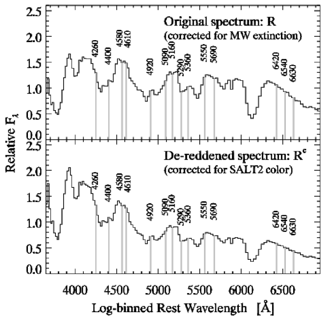
We use the same binning as Bailey et al. (2009), namely 134 bins equally spaced in $\ln\lambda$ between 3500 Å and 8500 Å (rest frame), although most of the CfA spectra used here do not extend beyond $\sim 7100$ Å (see § 4.3). The resulting $\sim 2000$   km  s^-1 bin size is significantly less than the typical width of a SN Ia feature ($\sim 10000$   km  s^-1). The error on $\mathcal{R}$ includes a flux error (from the corresponding variance spectrum), an error due to the relative flux calibration accuracy (see § 4.2), and an error due to the SALT2 color precision. When there are several spectra of a given SN Ia within $\Delta t=2.5$ d of the age we consider (see § 4.3 for spectra at maximum light; § 4.4 for spectra at other ages), we use the error-weighted mean and standard deviation of all flux ratios as our measurement and error, respectively. Bailey et al. (2009) also chose $\Delta t=2.5$ d in their analysis, and we find that increasing $\Delta t$ worsens the results while decreasing it leads to too small a sample.

Bailey et al. (2009) cross-checked the results for their best single flux ratio $\mathcal{R}(6420/4430)$ using the the sample of SN Ia spectra published by Matheson et al. (2008) [and available through the CfA SN Archive]. We checked the validity of our flux ratio measurements by comparing the values of $\mathcal{R}(6420/4430)$ in the Matheson et al. (2008) sample with those reported in Table 2 of Bailey et al. (2009). In all cases, our measurements agree well within the $1\sigma$ errors. This also holds for SN 1998bu, accidentally removed from the Matheson et al. (2008) sample by Bailey et al. (2009) [H. Fakhouri 2010, private communication]. We note that we were unable to cross-check the flux ratio measurements of Bailey et al. (2009) in a similar fashion, since none of their 58 SN Ia spectra are publicly available.

4.2 Impact of relative flux calibration and SALT2 color

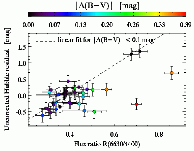
When the $\lambda_{X}$ and $\lambda_{Y}$ wavelength bins have a large separation ($\gtrsim 1000$ Å), $\mathcal{R}(\lambda_{X}/\lambda_{Y})$ is essentially a color measurement. We therefore expect flux ratios to be sensitive to the relative flux calibration accuracy of the spectra. Fig. 2 shows the relation between uncorrected Hubble residuals [i.e. $m_{B}-M-\mu(z)$] and our most highly-ranked flux ratio $\mathcal{R}(6630/4400)$ at maximum light (see § 4.3). There is one data point per SN Ia, color-coded according to the absolute difference in $B-V$ color at maximum light derived from the spectrum and that derived from the photometry, noted $|\Delta(B-V)|$, which we use as a proxy for relative flux calibration accuracy. The bulk of the sample defines a highly correlated relation (dashed line), with several outliers all having $|\Delta(B-V)|\geq 0.1$ mag. We therefore restrict our analysis to SN Ia with spectra that have a relative flux calibration better than 0.1 mag.

Figure 2: Uncorrected Hubble residual vs. flux ratio $\mathcal{R}(6630/4400)$ at maximum light, color-coded according to the absolute difference in $B-V$ color derived from the spectrum and that derived from the photometry, noted $|\Delta(B-V)|$. The dashed line is a linear fit to the SN Ia with $|\Delta(B-V)|<0.1$ mag. The highly-reddened SN 2006br is not shown here.

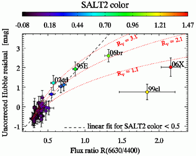
Bailey et al. (2009) noted that the highly-reddened SN 1999cl was a large outlier in their analysis, and attributed this to the non-standard nature of the extinction towards this SN ($R_{V}\approx 1.5$; Krisciunas et al. 2006). To explore the effects of reddening, in Fig. 3 (left), we show the relation between uncorrected Hubble residual and $\mathcal{R}(6630/4400)$ at maximum light, for SN Ia at redshifts $z>0.005$ that satisfy our requirement on the relative flux calibration accuracy. Using this lower redshift bound has the effect of including several highly-reddened SN Ia (including SN 1999cl; see Fig. 4), which are otherwise excluded based on the redshift cut we use elsewhere this paper ($z>0.015$). For SN Ia with $c<0.5$, $\mathcal{R}(6630/4400)$ is highly correlated with uncorrected Hubble residuals, but those with red colors ($c>0.5$) tend to deviate significantly from this relation (dashed line; this is not the case for SN 1995E, for which $c\approx 0.9$), the two largest outliers corresponding to the reddest SN Ia (SN 1999cl and SN 2006X). Both are subject to high extinction by non-standard dust in their respective host galaxies ($A_{V}\approx 2$ mag for $R_{V}\approx 1.5$; Krisciunas et al. 2006; Wang et al. 2008) and display time-variable Na I D absorption, whose circumstellar or interstellar origin is still debated (Patat et al. 2007; Blondin et al. 2009). The reddening curves in Fig. 3 (dotted lines) seem to corroborate the fact that the nonlinear increase of flux ratios at high values of the SALT2 color parameter is mainly due to reddening by dust with low $R_{V}$. Nonetheless, SN 1999cl still stands out in this respect as it would require a value of $R_{V}\lesssim 0.5$ inconsistent with that found by Krisciunas et al. (2006). Moreover, while we obtain consistent $R_{V}$ estimates for SN 2006X using other flux ratios, this is not the case for SN 2006br, for which some flux ratios are consistent with $R_{V}=3.1$.

Figure 3: Left: Uncorrected Hubble residual vs. flux ratio $\mathcal{R}(6630/4400)$ at maximum light for SN Ia at $z>0.005$ with $|\Delta(B-V)|<0.1$ mag, color-coded according to the SALT2 color parameter, $c$. Points corresponding to SN Ia with $c>0.5$ are labeled. The dashed line is a linear fit to the SN Ia with $c<0.5$. The dotted lines are reddening curves for different values of $R_{V}$, normalized to the smallest $\mathcal{R}(6630/4400)$ value. Right: Color-corrected Hubble residual vs. color-corrected flux ratio $\mathcal{R}^{c}(6420/5290)$ at maximum light.

Figure 4: Histogram of the SALT2 color parameter ($c$) for SN Ia at $z>0.015$ (open) and $0.005<z<0.015$ (hatched). Bins that include SN Ia with $c>0.5$ are labeled.

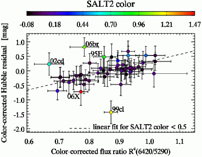
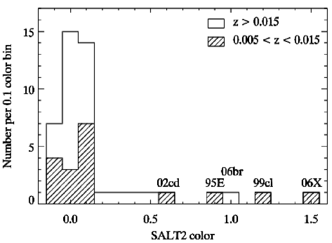
The right panel of Fig. 3 shows the relation between color-corrected Hubble residual [i.e. $m_{B}-M-\beta c-\mu(z)$] and our most highly-ranked color-corrected flux ratio $\mathcal{R}^{c}(6420/5290)$ at maximum light (see § 4.3) for the same sample. SN Ia with a SALT2 color $c>0.5$ are again outliers. As noted by Bailey et al. 2009, this shows that a single color parameter cannot encompass the variety of SN Ia intrinsic colors and extinction by non-standard dust. We therefore impose a cut on SALT2 color in our analysis, only considering SN Ia with $c<0.5$. Four of the five SNe with $c>0.5$ in Fig. 3 are rejected anyway based on our redshift cut. The remaining one, SN 2006br, is then rejected based on our color cut.

4.3 Results on Maximum-light Spectra

4.3.1 Selecting the best flux ratios

After selecting SN Ia that satisfy both requirements on relative flux calibration accuracy and SALT2 color parameter, we are left with 26 SN Ia at $z>0.015$ with spectra within $\Delta t=2.5$ d from maximum light (see Table 1, where we also present selected flux ratio measurements). The spectra show no sign of significant contamination by host-galaxy light, which can also bias the flux ratio measurements. We make no cut based on the signal-to-noise ratio (S/N) of our spectra, as they are generally well in excess of 100 per log-wavelength bin. We only consider flux ratios for wavelength bins represented in all the spectra. This leads to 98 bins between $\sim 3690$ Å and $\sim 7060$ Å, i.e. 9506 independent flux ratios.

Table 1: SN Ia sample for flux ratio measurements at maximum light

SN	$z_{\rm CMB}$	$m_{B}$	$x_{1}$	$c$	$\mathcal{R}(6630/4400)$	$\mathcal{R}^{c}(6420/5290)$	$\mathcal{R}^{c}(5690/5360)$	$\mathcal{R}^{c}(5160/5290)$	$\mathcal{R}^{c}(5690/5550)$
1998V	0.0170	15.085 (0.020)	$-0.435$ (0.161)	$0.031$ (0.015)	0.330 (0.005)	0.744 (0.006)	1.045 (0.004)	1.485 (0.006)	0.933 (0.004)
1998dx	0.0539	17.536 (0.037)	$-1.890$ (0.457)	$-0.051$ (0.027)	0.365 (0.018)	0.949 (0.027)	1.086 (0.024)	1.445 (0.033)	0.946 (0.018)
1998eg	0.0237	16.096 (0.016)	$-0.956$ (0.366)	$0.048$ (0.019)	0.378 (0.023)	0.920 (0.022)	1.070 (0.011)	1.478 (0.013)	0.995 (0.007)
1999aa	0.0152	14.698 (0.009)	$0.896$ (0.073)	$-0.019$ (0.009)	0.286 (0.027)	0.704 (0.025)	1.054 (0.012)	1.448 (0.011)	0.994 (0.006)
1999cc	0.0316	16.760 (0.010)	$-1.891$ (0.175)	$0.057$ (0.012)	0.406 (0.013)	0.994 (0.017)	1.001 (0.015)	1.513 (0.019)	0.850 (0.011)
1999ek	0.0176	15.587 (0.009)	$-1.075$ (0.127)	$0.163$ (0.010)	0.478 (0.039)	0.936 (0.036)	1.091 (0.016)	1.461 (0.014)	0.952 (0.007)
1999gd	0.0191	16.940 (0.022)	$-1.210$ (0.193)	$0.455$ (0.022)	0.714 (0.013)	0.929 (0.016)	1.081 (0.024)	1.455 (0.020)	1.028 (0.015)
2000dk	0.0165	15.347 (0.021)	$-2.658$ (0.301)	$0.055$ (0.022)	0.423 (0.017)	0.933 (0.017)	1.038 (0.009)	1.425 (0.010)	1.006 (0.006)
2000fa	0.0218	15.883 (0.023)	$0.311$ (0.127)	$0.100$ (0.018)	0.410 (0.046)	0.829 (0.042)	1.082 (0.020)	1.459 (0.017)	0.902 (0.009)
2001eh	0.0363	16.575 (0.018)	$1.457$ (0.222)	$0.020$ (0.017)	0.312 (0.047)	0.799 (0.043)	1.040 (0.020)	1.451 (0.019)	0.931 (0.010)
2002ck	0.0302	16.303 (0.048)	$-0.183$ (0.147)	$-0.017$ (0.023)	0.348 (0.046)	0.752 (0.042)	1.030 (0.020)	1.463 (0.017)	0.945 (0.010)
2002hd	0.0360	16.738 (0.038)	$-0.748$ (0.456)	$0.100$ (0.022)	0.403 (0.027)	0.748 (0.027)	0.955 (0.018)	1.378 (0.020)	0.899 (0.013)
2002hu	0.0359	16.587 (0.012)	$0.052$ (0.143)	$-0.052$ (0.012)	0.293 (0.027)	0.768 (0.029)	1.048 (0.021)	1.509 (0.029)	0.984 (0.017)
2002jy	0.0187	15.702 (0.019)	$0.660$ (0.212)	$0.013$ (0.015)	0.305 (0.015)	0.795 (0.015)	1.073 (0.010)	1.566 (0.012)	0.963 (0.007)
2002kf	0.0195	15.654 (0.033)	$-1.493$ (0.189)	$0.009$ (0.023)	0.361 (0.035)	0.953 (0.035)	1.132 (0.024)	1.550 (0.024)	0.969 (0.014)
2003U	0.0279	16.471 (0.046)	$-2.536$ (0.558)	$0.033$ (0.035)	0.373 (0.009)	0.891 (0.016)	1.048 (0.016)	1.445 (0.025)	0.965 (0.014)
2003ch	0.0256	16.659 (0.022)	$-1.655$ (0.297)	$0.012$ (0.019)	0.402 (0.025)	1.024 (0.024)	1.218 (0.010)	1.570 (0.009)	1.043 (0.005)
2003it	0.0240	16.342 (0.028)	$-1.815$ (0.359)	$0.084$ (0.029)	0.432 (0.011)	0.918 (0.011)	1.087 (0.007)	1.456 (0.009)	0.950 (0.005)
2003iv	0.0335	16.961 (0.026)	$-2.473$ (0.486)	$-0.031$ (0.028)	0.420 (0.005)	1.092 (0.011)	1.081 (0.011)	1.467 (0.015)	0.940 (0.009)
2004as	0.0321	16.956 (0.018)	$-0.017$ (0.206)	$0.128$ (0.016)	0.415 (0.006)	0.838 (0.008)	1.065 (0.009)	1.573 (0.011)	0.975 (0.007)
2005ki	0.0208	15.551 (0.029)	$-2.123$ (0.153)	$-0.059$ (0.026)	0.398 (0.032)	0.975 (0.030)	1.091 (0.015)	1.441 (0.015)	0.957 (0.009)
2006ax	0.0180	15.010 (0.010)	$-0.062$ (0.062)	$-0.049$ (0.009)	0.304 (0.019)	0.851 (0.018)	1.082 (0.008)	1.558 (0.009)	1.009 (0.005)
2006gj	0.0277	17.668 (0.033)	$-2.073$ (0.280)	$0.409$ (0.023)	0.675 (0.008)	0.988 (0.012)	1.011 (0.011)	1.377 (0.014)	0.930 (0.009)
2006sr	0.0232	16.126 (0.017)	$-1.754$ (0.220)	$0.060$ (0.015)	0.422 (0.019)	0.939 (0.018)	1.031 (0.010)	1.474 (0.010)	0.913 (0.006)
2007ca	0.0151	15.933 (0.013)	$0.289$ (0.122)	$0.305$ (0.012)	0.547 (0.028)	0.895 (0.026)	1.097 (0.012)	1.569 (0.012)	0.986 (0.006)
2008bf	0.0257	15.703 (0.010)	$0.097$ (0.095)	$0.031$ (0.010)	0.315 (0.038)	0.806 (0.035)	1.047 (0.016)	1.526 (0.013)	0.924 (0.007)

We run the $K$-fold cross-validation procedure outlined in § 2.3, and consider the five models for estimating distances to SN Ia described in § 1:

$$\mu = m_{B}-M+\gamma\mathcal{R}$$ (9)

$$\mu = m_{B}-M+\alpha x_{1}+\gamma\mathcal{R}$$ (10)

$$\mu = m_{B}-M-\beta c+\gamma\mathcal{R}^{c}$$ (11)

$$\mu = m_{B}-M+\alpha x_{1}-\beta c+\gamma\mathcal{R}^{c}$$ (12)

$$\mu = m_{B}-M+\alpha x_{1}-\beta c.$$ (13)

When no color correction is involved (Eqs. 9-10), we use the uncorrected flux ratio $\mathcal{R}$. When a color correction is involved (the $-\beta c$ term in Eqs. 11-12), we use the color-corrected version of the flux ratio $\mathcal{R}^{c}$. Using $\mathcal{R}$ in combination with color, or $\mathcal{R}^{c}$ alone or in combination with $x_{1}$, severely degrades the predictive power of the model, so we do not report results using $(c,\mathcal{R})$; $\mathcal{R}^{c}$ alone; or $(x_{1},\mathcal{R}^{c})$.

We rank the flux ratios in each case based on the intrinsic prediction error ($\sigma_{\rm pred}$; see § 2.4), but note that ranking based on the weighted rms of prediction Hubble residuals makes almost no difference. The results for the top five flux ratios are displayed in Table 2. We also report the best-fit $\gamma$, the weighted rms of prediction Hubble residuals (WRMS), the intrinsic correlation of residuals with those found using the standard $(x_{1},c)$ predictors (noted $\rho_{x_{1},c}$; see § 2.4), and the difference in intrinsic prediction error with respect to the standard $(x_{1},c)$ model, noted $\Delta_{x_{1},c}$. Since we compute the error on $\Delta_{x_{1},c}$ (see Appendix B), we also report the significance of this difference with respect to the standard $(x_{1},c)$ predictors. This is a direct measure of whether a particular model predicts more accurate distances to SN Ia when compared to the standard approach, and if so how significant is the improvement. Fig. 5 shows the resulting Hubble diagram residuals vs. redshift for the best flux ratio in each of the four models given by Eqs. 9-12, and using the standard $(x_{1},c)$ predictors.

Table 2: Top 5 flux ratios at maximum light from 10-fold CV on 26 SN Ia

Rank	$\lambda_{X}$	$\lambda_{Y}$	$\gamma$	WRMS	$\sigma_{\rm pred}$	$\rho_{x_{1},c}$	$\Delta_{x_{1},c}$
$\mathcal{R}$
1	6630	4400	$-4.37\pm 0.09$	$0.189\pm 0.026$	$0.163\pm 0.030$	$0.80\pm 0.09$	$-0.018\pm 0.025\ (0.7\sigma)$
2	6630	4430	$-4.44\pm 0.12$	$0.191\pm 0.027$	$0.166\pm 0.030$	$0.60\pm 0.15$	$-0.015\pm 0.033\ (0.5\sigma)$
3	6630	4670	$-5.16\pm 0.11$	$0.197\pm 0.027$	$0.171\pm 0.031$	$0.57\pm 0.17$	$-0.007\pm 0.032\ (0.2\sigma)$
4	6900	4460	$-5.71\pm 0.12$	$0.196\pm 0.027$	$0.171\pm 0.031$	$0.54\pm 0.17$	$-0.009\pm 0.036\ (0.2\sigma)$
5	6420	4430	$-3.40\pm 0.10$	$0.196\pm 0.028$	$0.173\pm 0.031$	$0.56\pm 0.16$	$-0.010\pm 0.033\ (0.3\sigma)$
$(x_{1},\mathcal{R})$
1	6630	4400	$-4.51\pm 0.15$	$0.201\pm 0.028$	$0.176\pm 0.032$	$0.74\pm 0.10$	$-0.006\pm 0.028\ (0.2\sigma)$
2	6630	4430	$-4.57\pm 0.20$	$0.204\pm 0.029$	$0.180\pm 0.032$	$0.55\pm 0.17$	$-0.001\pm 0.033\ (0.0\sigma)$
3	6900	4460	$-5.81\pm 0.16$	$0.206\pm 0.029$	$0.182\pm 0.032$	$0.52\pm 0.17$	$0.002\pm 0.032\ (0.1\sigma)$
4	6900	4370	$-4.46\pm 0.04$	$0.206\pm 0.029$	$0.182\pm 0.032$	$0.69\pm 0.13$	$0.001\pm 0.030\ (0.0\sigma)$
5	6990	4370	$-4.95\pm 0.05$	$0.207\pm 0.029$	$0.183\pm 0.032$	$0.61\pm 0.15$	$0.003\pm 0.035\ (0.1\sigma)$
$(c,\mathcal{R}^{c})$
1	6420	5290	$-1.75\pm 0.10$	$0.175\pm 0.025$	$0.148\pm 0.029$	$0.80\pm 0.09$	$-0.032\pm 0.023\ (1.4\sigma)$
2	6630	4890	$-2.19\pm 0.14$	$0.181\pm 0.024$	$0.148\pm 0.031$	$0.81\pm 0.08$	$-0.023\pm 0.022\ (1.0\sigma)$
3	4890	6630	$0.73\pm 0.06$	$0.182\pm 0.024$	$0.148\pm 0.031$	$0.83\pm 0.08$	$-0.023\pm 0.023\ (1.0\sigma)$
4	4890	6810	$0.60\pm 0.05$	$0.180\pm 0.024$	$0.148\pm 0.030$	$0.73\pm 0.11$	$-0.026\pm 0.026\ (1.0\sigma)$
5	6540	4890	$-1.84\pm 0.12$	$0.179\pm 0.024$	$0.149\pm 0.030$	$0.88\pm 0.05$	$-0.026\pm 0.020\ (1.3\sigma)$
$(x_{1},c,\mathcal{R}^{c})$
1	5690	5360	$-2.78\pm 0.20$	$0.164\pm 0.023$	$0.134\pm 0.028$	$0.69\pm 0.13$	$-0.044\pm 0.028\ (1.6\sigma)$
2	5360	5690	$3.23\pm 0.25$	$0.167\pm 0.023$	$0.137\pm 0.028$	$0.69\pm 0.13$	$-0.042\pm 0.028\ (1.5\sigma)$
3	5660	5290	$-1.95\pm 0.24$	$0.173\pm 0.024$	$0.142\pm 0.029$	$0.72\pm 0.11$	$-0.038\pm 0.029\ (1.3\sigma)$
4	5690	5290	$-1.67\pm 0.21$	$0.171\pm 0.024$	$0.142\pm 0.028$	$0.75\pm 0.11$	$-0.037\pm 0.022\ (1.7\sigma)$
5	5290	5660	$2.75\pm 0.33$	$0.174\pm 0.024$	$0.144\pm 0.029$	$0.73\pm 0.11$	$-0.036\pm 0.028\ (1.3\sigma)$
$(x_{1},c)$
$\cdots$	$\cdots$	$\cdots$	$\cdots$	$0.204\pm 0.029$	$0.181\pm 0.032$	$\cdots$	$\cdots$

Figure 5: Hubble diagram residuals for the highest-ranked flux ratios at maximum light. From top to bottom: prediction residuals using $\mathcal{R}$ only; $(\mathcal{R},x_{1})$; $(\mathcal{R}^{c},c)$; $(\mathcal{R}^{c},x_{1},c)$; and using the standard SALT2 fit parameters $(x_{1},c)$. In each case we indicate the weighted rms of prediction Hubble residuals (gray highlighted region).

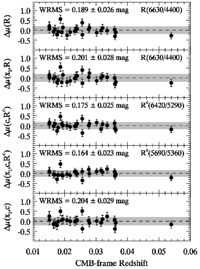
All the flux ratios listed in Table 2 lead to an improvement over the standard $(x_{1},c)$ correction (i.e. $\Delta_{x_{1},c}<0$), as found by Bailey et al. (2009), but the significance is low: $<1\sigma$ for $\mathcal{R}$ only; $\ll 1\sigma$ for $(x_{1},\mathcal{R})$; $\sim 1.5\sigma$ for $(c,\mathcal{R}^{c})$ and $(x_{1},c,\mathcal{R}^{c})$. This is in part due to the small number of SN Ia in our sample. Note that $\rho_{x_{1},c}>0.5$ in all cases, i.e. the models that include a flux ratio tend to make prediction errors in the same direction as $(x_{1},c)$, and we do not expect to gain much by combining these models.

Using best single flux ratio $\mathcal{R}(6630/4400)$ by itself reduces the weighted rms of prediction residuals (as well as the intrinsic prediction error, $\sigma_{\rm pred}$) by $\lesssim 10$% when compared with $(x_{1},c)$ [${\rm WRMS}=0.189\pm 0.026$ mag cf. $0.204\pm 0.029$ mag], although as noted above the significance of the difference in intrinsic prediction error is negligible ($\Delta_{x_{1},c}=-0.018\pm 0.025$ mag, or $0.7\sigma$).

Using $\mathcal{R}$ in combination with $x_{1}$ leads to no improvement over using $\mathcal{R}$ alone (although this is not reported by Bailey et al. 2009, it is consistent with their findings; S. Bailey 2009, private communication), and even leads to systematically worse results. Our best single flux ratio $\mathcal{R}(6630/4400)$ yields a difference in intrinsic prediction error with respect to $(x_{1},c)$ of $\Delta_{x_{1},c}=-0.018\pm 0.025$ mag, when used on its own, while it yields $\Delta_{x_{1},c}=-0.006\pm 0.028$ mag when combined with $x_{1}$. These differences are statistically indistinguishable from one another given the size of the error on $\Delta_{x_{1},c}$, but they are systematic regardless of the flux ratio we consider.

This seems counter-intuitive, as one might expect that including an additional predictor would result in more accurate distance predictions. However, this is not necessarily the case under cross-validation. The reason is that $x_{1}$ by itself is a poor predictor of Hubble residuals, and one does not gain anything by combining it with $\mathcal{R}(6630/4400)$. This is not surprising, as the relation between light-curve width and luminosity is only valid if the SN Ia are corrected for color or extinction by dust beforehand. In fact, $\mathcal{R}(6630/4400)$ by itself accounts for most of the variation in Hubble residuals. When we cross-validate, the extra coefficient $\alpha$ will tend to fit some noise in a given training set, and this relation will not generalize to the validation set. This results in an increase in prediction error because the added information is not useful. We see from Table 2 that adding $x_{1}$ affects the best-fit value for $\gamma$ [$\gamma=-4.51\pm 0.15$ cf. $-4.37\pm 0.09$ for $\mathcal{R}(6630/4400)$ only]; moreover, we obtain $\alpha\lesssim 0$ when using $[x_{1},\mathcal{R}(6630/4400)]$ where $\alpha\approx 0.15$ when using $(x_{1},c)$, which again shows that $\alpha$ is fitting noise when $\mathcal{R}(6630/4400)$ is combined with $x_{1}$. This illustrates the advantage of using cross-validation in guarding against over-fitting noise as more parameters and potential predictors are added.

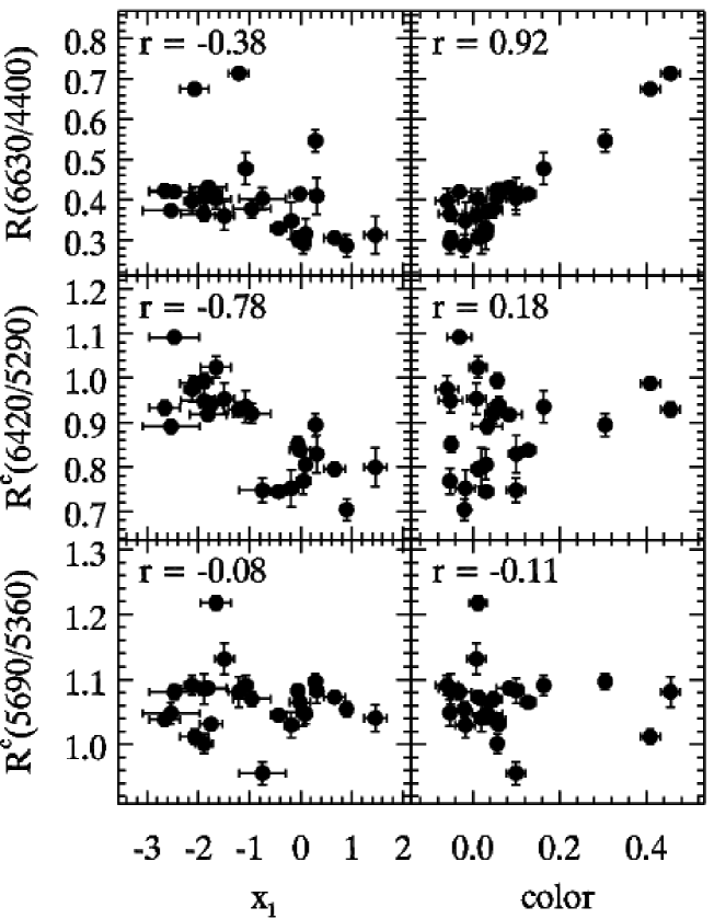
Figure 6 (upper panel) shows why $\mathcal{R}(6630/4400)$ alone is a good predictor of Hubble residuals. Its strong correlation with SALT2 color (Pearson correlation coefficient $r=0.92$) shows that this ratio is essentially a color measurement. The correlation with $x_{1}$ is less pronounced ($r=-0.38$), but this is largely due to a small number of outliers: removing the three largest outliers results in a Pearson correlation coefficient $r=-0.65$. The flux ratio $\mathcal{R}(6630/4400)$ by itself is thus as useful a predictor as $x_{1}$ and $c$ combined.

The relation between $\mathcal{R}(6630/4400)$ and $x_{1}$ is not linear, but it is certainly true that SN Ia with higher $x_{1}$ (i.e. broader light curves) tend to have lower $\mathcal{R}(6630/4400)$ [the same is true for $\mathcal{R}(6420/4430)$, the highest-ranked flux ratio by Bailey et al. 2009]. Since the width of the lightcurve is a parameter intrinsic to each SN Ia (although its measurement can be subtly affected by host-galaxy reddening; see Phillips et al. 1999), the correlation between $x_{1}$ and $\mathcal{R}(6630/4400)$ shows that the color variation measured by $\mathcal{R}(6630/4400)$ is intrinsic in part. This is consistent with the so-called “brighter-bluer” relation of Tripp (1998): overluminous SN Ia are intrinsically bluer than underluminous SN Ia (see also Riess et al. 1996).

Using a color-corrected flux ratio $\mathcal{R}^{c}$ in combination with color results in even lower Hubble residual scatter when compared with the single flux ratio case. Our best flux ratio in this case, $\mathcal{R}^{c}(6420/5290)$, reduces the weighted rms of prediction residuals by $\sim 15$% with respect to $(x_{1},c)$ [${\rm WRMS}=0.175\pm 0.025$ mag cf. $0.204\pm 0.029$ mag], and the intrinsic prediction error by $\sim 20$% [$\sigma_{\rm pred}=0.148\pm 0.029$ mag cf. $0.181\pm 0.032$ mag]. Again, the significance of this difference is only $1.4\sigma$ ($\Delta_{x_{1},c}=-0.032\pm 0.023$ mag). We see from Fig. 6 (middle panel) that $\mathcal{R}^{c}(6420/5290)$ is strongly anti-correlated with $x_{1}$ ($r=-0.78$), and that dereddening the spectra using the SALT2 color law is effective in removing any dependence of $\mathcal{R}^{c}(6420/5290)$ on color, as expected.

Figure 6: Correlation between the highest-ranked $(\mathcal{R},\mathcal{R}^{c})$ at maximum light and the SALT2 fit parameters $(x_{1},c)$.

One would naively think that combining our best color-corrected ratio $\mathcal{R}^{c}(6420/5290)$ with $(x_{1},c)$ would lead to an even further improvement, but this is not the case. In fact, $\mathcal{R}^{c}(6420/5290)$ ranks 298^th when we consider the set of predictors $(x_{1},c,\mathcal{R}^{c})$. This is due to the strong anti-correlation of $\mathcal{R}^{c}(6420/5290)$ with $x_{1}$. Adding $x_{1}$ as an extra predictor when $\mathcal{R}^{c}(6420/5290)$ already includes this information means $\alpha$ will tend to fit noise in a given training set, as was the case for the set of $(x_{1},\mathcal{R})$ predictors when compared with $\mathcal{R}$-only. Indeed, the best-fit value for $\alpha$ for $[x_{1},c,\mathcal{R}^{c}(6420/5290)]$ is again consistent with 0.

Nonetheless, several color-corrected flux ratios do result in a further reduced scatter when combined with $(x_{1},c)$, although the wavelength baseline for these ratios is much smaller ($\lesssim 400$ Å) and the wavelength bins forming the ratios are all concentrated in the region of the S II $\lambda$$\lambda$5454,5640 doublet. Our highest-ranked flux ratio in this case, $\mathcal{R}^{c}(5690/5360)$, reduces the weighted rms of prediction residuals by $\sim 20$% with respect to $(x_{1},c)$ [${\rm WRMS}=0.164\pm 0.023$ mag cf. $0.204\pm 0.029$ mag], and the intrinsic prediction error by $\sim 25$% [$\sigma_{\rm pred}=0.134\pm 0.028$ cf. $0.181\pm 0.032$ mag]. Again, the significance of this difference is only $1.6\sigma$ ($\Delta_{x_{1},c}=-0.044\pm 0.028$ mag). We see from Fig. 6 (lower panel) that this ratio is not correlated with $x_{1}$ ($r=-0.08$) or $c$ ($r=0.11$), and thus constitutes a useful additional predictor of distances to SN Ia.

4.3.2 Two-dimensional maps of all flux ratios

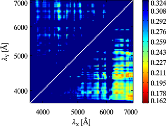
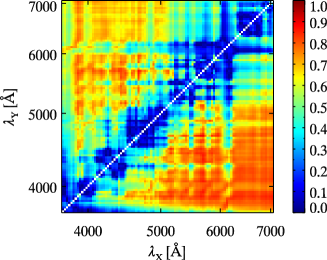
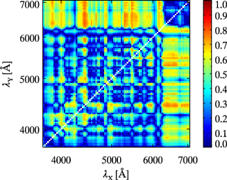
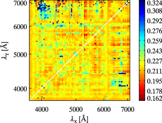
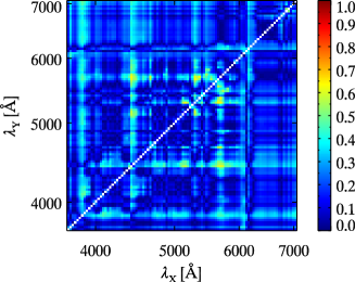
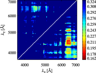
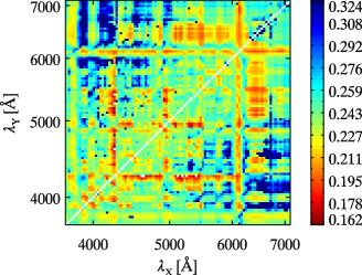
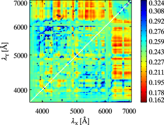
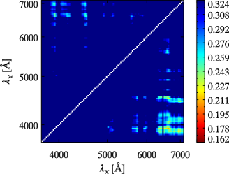
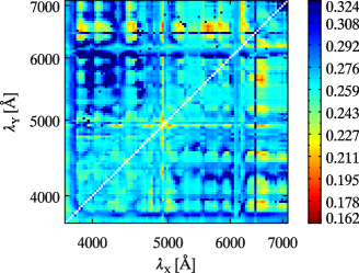
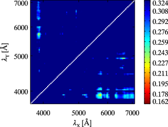
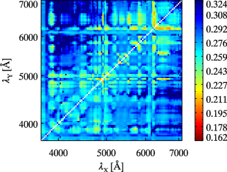
The results for all 9506 flux ratios are displayed in Fig. 7. The four rows correspond to the four models for estimating SN Ia distances that include a flux ratio (Eqs. 9-12). The left column is color-coded according to the weighted rms of prediction Hubble residuals (flux ratios that result in ${\rm WRMS}>0.324$ mag are given the color corresponding to ${\rm WRMS}=0.324$ mag), while the right column is color-coded according to the absolute Pearson correlation coefficient of the correction terms with uncorrected Hubble residuals [e.g. for the set of predictors $(c,\mathcal{R}^{c})$, the correlation of $(-\beta c+\gamma\mathcal{R}^{c})$ with uncorrected residuals].

	WRMS residuals   [mag]	Absolute Pearson correlation
$\mathcal{R}$
$(x_{1},\mathcal{R})$
$(c,\mathcal{R}^{c})$
$(x_{1},c,\mathcal{R}^{c})$

Figure 7: Results from 10-fold cross-validation on maximum-light spectra. From top to bottom: $\mathcal{R}$ only; ($x_{1},\mathcal{R}$); ($c,\mathcal{R}^{c}$); ($x_{1},c,\mathcal{R}^{c}$). The left column is color-coded according to the weighted rms of prediction Hubble residuals, while the right column corresponds to the absolute Pearson cross-correlation coefficient of the correction terms with uncorrected Hubble residuals.

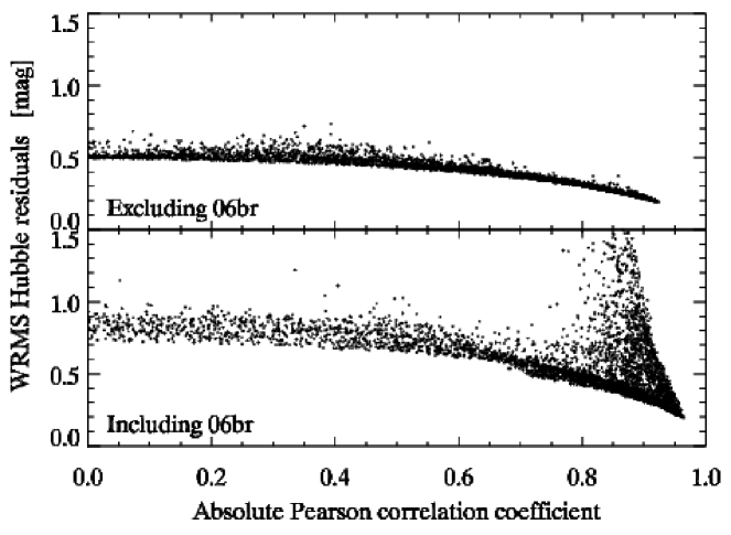
Only a very restricted number of wavelength bins lead to a low WRMS of prediction Hubble residuals when a flux ratio $\mathcal{R}$ is used by itself (Fig. 7; upper left), namely $\lambda_{X}\gtrsim 6300$ Å and $\lambda_{Y}\approx 4400$ Å (4 of the 5 best flux ratios in Table 2 for $\mathcal{R}$-only have $\lambda_{Y}\approx 4400$ Å). This is in stark contrast with the large number of flux ratios with absolute Pearson correlation coefficients $|r|>0.8$ (Fig. 7; upper right). In general, a flux ratio with a higher correlation coefficient will result in a Hubble diagram with less scatter, but this is not systematically the case, and the relation between the two is certainly not linear. For Pearson correlation coefficients $|r|>0.8$, the standard deviation of Hubble residuals can vary by up to 0.1 mag at any given $|r|$ (Fig. 8, top panel). This is because the cross-correlation coefficient does not take into account errors on $\mathcal{R}$ or on the Hubble residual, and is biased by outliers and reddened SN Ia. The lower panel of Fig. 8 shows the impact of including the highly-reddened SN 2006br: at any given $|r|$, the resulting weighted rms of prediction Hubble residuals is 30-60% higher. Moreover, many flux ratios with high correlation coefficients ($|r|>0.8$) result in Hubble diagrams with excessively large scatter (${\rm WRMS}>1$ mag). This is counter-intuitive, since the resulting scatter in these cases appears to be larger than when no predictors at all are used to determine distances to SN Ia (in which case ${\rm WRMS}\approx 0.5$ mag). The reason is that we consider the scatter under cross-validation, as opposed to fitting all the SN Ia at the same time. In these aberrant cases, the trained model is sensitive to the inclusion or exclusion of some outlier in the training set, and this leads to large errors when the outlier is in the validation set. Last, including this SN leads to correlations with $|r|>0.95$, where there are none otherwise. Fig. 8 thus justifies our excluding SN 2006br from the sample (already excluded based on our cut on SALT2 color; see § 4.2), and illustrates the advantage of selecting flux ratios based directly on the weighted rms of prediction Hubble diagram residuals, rather than on cross-correlation coefficients. As already mentioned in § 4.3.1, using cross-validated prediction errors to select the best flux ratios guards us against overfitting a small sample: in the naive approach that consists in fitting the entire SN Ia sample at once, adding more predictors always leads to a lower scatter in Hubble residuals (this is known as “resubstitution”; see, e.g., Mandel et al. 2009).

Figure 8: Weighted rms of prediction Hubble residuals vs. absolute Pearson cross-correlation coefficient for all flux ratios at maximum light, excluding (top) and including (bottom) the highly-reddened SN 2006br.

When the SALT2 color parameter is used in combination with a color-corrected flux ratio $\mathcal{R}^{c}$, there are again restricted wavelength regions that lead to a low weighted rms of prediction Hubble residuals (Fig. 7; third row left) [4 of the 5 best flux ratios in Table 2 for $(c,\mathcal{R}^{c})$ predictors involve wavelength bins at $\sim 4900$ Å and $\sim 6500$ Å]. The SALT2 color parameter $c$ does not attempt to distinguish between reddening by dust and intrinsic color variations. Dereddening the spectra using this parameter corrects for both effects regardless of their relative importance. However, since the SALT2 color law is very similar to the Cardelli et al. (1989) extinction law with $R_{V}=3.1$ and $E(B-V)=0.1$ mag (Guy et al. 2007, their Fig. 3), one generally assumes that the color correction removes the bulk of reddening by dust, and the remaining variations in the SED are primarily intrinsic to the supernova. If this is so, it is intriguing that the best flux ratios for the $\mathcal{R}$-only and $(c,\mathcal{R}^{c})$ models share similar wavelength bins. The recent survey of 2D SN Ia models from Kasen et al. (2009) suggests that a significant part of the color variation measured by the $\mathcal{R}(6630/4400)$ is indeed intrinsic (see § 4.3.4).

The second row of Fig. 7 confirms that using the $x_{1}$ parameter in combination with a flux ratio results in a slight degradation in the weighted rms of prediction residuals, while the correlations with uncorrected Hubble residuals are degraded with respect to cases where $\mathcal{R}$ is used by itself. Last, the bottom row of Fig. 7 is a visual demonstration that $(x_{1},c,\mathcal{R}^{c})$ fares better than $(c,\mathcal{R}^{c})$ overall, although the best color-corrected flux ratios do not perform significantly better. We see from the right panel that the correlations of $(\alpha x_{1}-\beta c+\gamma\mathcal{R}^{c})$ with uncorrected residuals all have absolute Pearson correlation coefficients $|r|\lesssim 0.5$. The two regions at $\lambda_{X,Y}\approx 5300$ Å stand out in the 2D plot of WRMS residuals, and all the top color-corrected ratios for $(x_{1},c,\mathcal{R}^{c})$ include a wavelength bin in that region (which corresponds to the absorption trough of the S II $\lambda$5454 line).

4.3.3 Comparison with Bailey et al. (2009)

We confirm the basic result of Bailey et al. (2009) using an independent sample and a different cross-validation method: the use of a flux ratio alone or in combination with a color parameter results in a Hubble diagram with lower scatter when compared to the standard $(x_{1},c)$ model. Using a flux ratio alone, Bailey et al. (2009) find $\mathcal{R}(6420/4430)$ as their most highly-ranked ratio, while we find $\mathcal{R}(6630/4400)$ [see Table 2]. The wavelength bins are almost identical, and in any case $\mathcal{R}(6420/4430)$ is amongst our top 5 ratios. For this ratio we find $\gamma=-3.40\pm 0.10$, in agreement with $\gamma=-3.5\pm 0.2$ found by Bailey et al. (2009).

The other four flux ratios given by Bailey et al. (2009) [their Table 1] are not part of our top-5 $\mathcal{R}$. For two of these ratios the reason is trivial: they include wavelength bins redder than 7100 Å, not covered by most of our spectra. The other two flux ratios [$\mathcal{R}(6420/4170)$ and $\mathcal{R}(6420/5120)$] lead to differences $<5$% on the Hubble diagram residual scatter with respect to the standard $(x_{1},c)$ model according to Bailey et al. (2009) [$\sigma=0.166\pm 0.016$ mag for $\mathcal{R}(6420/4170)$ and $\sigma=0.154\pm 0.015$ mag for $\mathcal{R}(6420/5120)$, cf. $0.161\pm 0.015$ mag for $(x_{1},c)$], and they rank 29^th and 658^th in our study, respectively. This discrepancy is in part due to the selection method: Bailey et al. (2009) select their best ratios based on cross-correlation coefficients with uncorrected magnitudes, while we select them based on the intrinsic prediction error from cross-validated Hubble diagram residuals. However, ranking our ratios using the same method as Bailey et al. (2009) does not resolve the discrepancy. It is possible that Bailey et al. (2009) are sensitive to their exact choice of training and validation samples, where we have randomized the approach. We note however that the impact on the weighted rms of prediction residuals is statistically indistinguishable for many flux ratios given our sample size (e.g. error on WRMS $\sim 0.03$ mag cf. differences of $\lesssim 0.01$ mag in WRMS for the top 5 flux ratios; see Table 2), so that the exact ranking of flux ratios is not well determined and subject to revisions from small changes in the input data.

Using both a color-corrected flux ratio $\mathcal{R}^{c}$ and the SALT2 color parameter decreases the residual scatter further, as found by Bailey et al. (2009). Using the set of predictors $[c,\mathcal{R}^{c}(6420/5290)]$ leads to $\sim 15$% lower WRMS with respect to $(x_{1},c)$ [${\rm WRMS}=0.175\pm 0.025$ mag cf. $0.204\pm 0.029$ mag], and to $\sim 20$% lower $\sigma_{\rm pred}$ [$\sigma_{\rm pred}=0.148\pm 0.029$ mag cf. $0.181\pm 0.032$ mag] at $1.4\sigma$ significance based on the difference in intrinsic prediction error, $\Delta_{x_{1},c}$. None of the color-corrected flux ratios listed by Bailey et al. (2009) [their Table 1] are part of our five highest-ranked $\mathcal{R}^{c}$, although our top ratios are formed with almost the same wavelength bins [$\mathcal{R}^{c}(6420/5290)$ in this paper; $\mathcal{R}^{c}(6420/5190)$ in Bailey et al. (2009)]. The other color-corrected ratios in Bailey et al. (2009) rank well below in our study, whether we select the best $\mathcal{R}^{c}$ according to the resulting Hubble residual scatter or the cross-correlation of $(-\beta c+\gamma\mathcal{R}^{c})$ with uncorrected residuals. The same caveats apply here as when selecting the best uncorrected flux ratios (see previous paragraph), although the $\mathcal{R}^{c}$ measurement is probably even more sensitive to the relative flux calibration accuracy of the spectra.

We also cross-checked the results of Bailey et al. (2009) by simply validating their best flux ratios on our entire SN Ia sample. The results are displayed in Table 3, where we give the weighted rms of Hubble residuals from a simultaneous fit to the entire SN Ia sample (as done by Bailey et al. 2009), as opposed to prediction residuals under cross-validation. For all flux ratios (both $\mathcal{R}$ and $\mathcal{R}^{c}$) in Table 3, our own best-fit $\gamma$ agrees within the $1\sigma$ errors with that found by Bailey et al. (2009) [noted $\gamma$(B09) in Table 3] , although we have systematically larger errors. We note that most of the top ratios reported by Bailey et al. (2009) lead to no significant improvement over $(x_{1},c)$, and even leads to slightly worse results for some ratios [e.g. $\mathcal{R}(6420/5120)$ results in ${\rm WRMS}=0.237\pm 0.032$ mag cf. $0.194\pm 0.027$ mag for $(x_{1},c)$]. A closer look at Table 1 of Bailey et al. (2009) shows that this is also the case in their paper: for the $\mathcal{R}$-only model, only one ratio out of five, namely $\mathcal{R}(6420/4430)$, results in a lower Hubble diagram residual scatter. The other four are either consistent with no improvement [$\mathcal{R}(7720/4370)$ and $\mathcal{R}(6420/5120)$], or yield slightly worse results [$\mathcal{R}(6420/4170)$ and $\mathcal{R}(7280/3980)$]. Again, this results from the way Bailey et al. (2009) selected their best ratios, based on the correlation with uncorrected Hubble residuals.

Table 3: Validation of top 5 flux ratios at maximum light from Bailey et al. (2009) [noted B09]

$\lambda_{\rm X}$	$\lambda_{\rm Y}$	$\gamma$	$\gamma$(B09)	WRMS	$\Delta_{x_{1},c}$
$\mathcal{R}$
6420	4430	$-3.40\pm 0.32$	$-3.5\pm 0.2$	$0.184\pm 0.026$	$-0.007\pm 0.031\ (0.2\sigma)$
6420	4170	$-4.43\pm 0.41$	$-4.9\pm 0.2$	$0.197\pm 0.028$	$0.008\pm 0.028\ (0.3\sigma)$
7720	4370	$\cdots$	$7.3\pm 0.3$	$\cdots$	$\cdots$
6420	5120	$-4.34\pm 0.42$	$-4.7\pm 0.3$	$0.237\pm 0.032$	$0.052\pm 0.034\ (1.5\sigma)$
7280	3980	$\cdots$	$7.9\pm 0.3$	$\cdots$	$\cdots$
$(c,\mathcal{R}^{c})$
6420	5190	$-2.20\pm 0.57$	$-3.5\pm 0.3$	$0.176\pm 0.025$	$-0.012\pm 0.016\ (0.8\sigma)$
5770	6420	$0.67\pm 0.22$	$1.4\pm 0.1$	$0.193\pm 0.027$	$0.005\pm 0.011\ (0.5\sigma)$
6420	5360	$-1.71\pm 0.43$	$-2.3\pm 0.2$	$0.169\pm 0.024$	$-0.019\pm 0.016\ (1.2\sigma)$
6760	6420	$1.79\pm 1.09$	$4.2\pm 0.5$	$0.217\pm 0.032$	$0.030\pm 0.025\ (1.2\sigma)$
6420	4430	$-2.56\pm 0.63$	$-3.2\pm 0.3$	$0.168\pm 0.024$	$-0.027\pm 0.023\ (1.2\sigma)$
$(x_{1},c)$
$\cdots$	$\cdots$	$\cdots$	$\cdots$	$0.194\pm 0.027$	$\cdots$

We cannot directly compare the resulting scatter in Hubble diagram residuals with those reported in Table 1 of Bailey et al. (2009). First, they use the sample standard deviation ($\sigma$), whereas we use the weighted rms (see § 2.4). Second, the scatter they find for the standard $(x_{1},c)$ model is significantly lower than ours. We have refit the data presented in Table 1 of Bailey et al. (2009) to derive the weighted rms of Hubble residuals for the $(x_{1},c)$ model from their sample, and find ${\rm WRMS}=0.148\pm 0.014$ mag, which is almost 0.05 mag smaller when compared to our sample ($0.194\pm 0.027$ mag). This difference in the Hubble residual scatter between the SN-Factory and CfA samples is consistent with the difference found amongst other nearby SN Ia samples by Hicken et al. (2009b).

Interestingly, using the WRMS statistic as opposed to the sample standard deviation results in a smaller difference in residual scatter between the $\mathcal{R}$-only and $(x_{1},c)$ models. Using our own fits of the data presented in Table 1 of Bailey et al. (2009), we find ${\rm WRMS}=0.131\pm 0.014$ mag for $\mathcal{R}(6420/4430)$, i.e. $\sim 11$% smaller scatter when compared to $(x_{1},c)$, where the difference between the two models is $\sim 20$% when considering the sample standard deviation.

4.3.4 Comparison with 2D models

We use synthetic spectra based on a recent 2D survey of delayed-detonation SN Ia models by Kasen et al. (2009) to investigate the physical origin of the high correlation between several flux ratios and uncorrected SN Ia magnitudes. These models were found to reproduce the empirical relation between peak $B$-band magnitude and post-maximum decline rate. A more detailed comparison of SN Ia data with these models will be presented elsewhere.

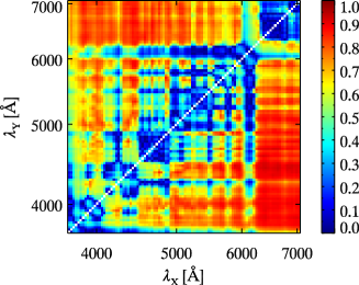
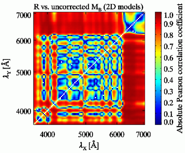
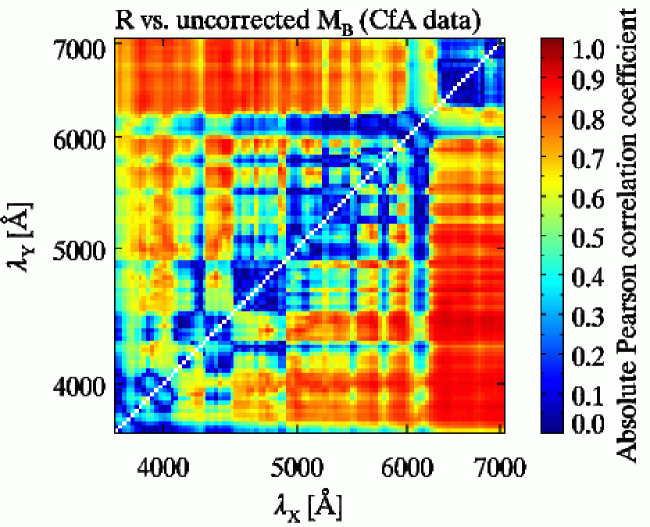
We measured flux ratios in the same manner as we did for our data, and computed Pearson correlation coefficients with (uncorrected) absolute magnitudes synthesized directly from the spectra. The 2D correlation map is shown in Fig. 9 (left panel), alongside the same map derived from the CfA SN Ia sample (right panel). At first glance, the two maps appear similar, with two large $\sim 1000$ Å-wide “bands” of flux ratios with strong correlations with uncorrected magnitudes, for $\lambda_{X}(\lambda_{Y})\gtrsim 6200$ Å and $\lambda_{Y}(\lambda_{X})\lesssim 6000$ Å, although the correlations are even stronger in the models (several flux ratios have absolute Pearson correlation coefficients $|r|>0.95$, where there are none in the data). A closer look reveals some important differences, the models having strong correlations for $6000$ Å$\lesssim\lambda_{X}(\lambda_{Y})\lesssim 6200$ Å and $\lambda_{Y}(\lambda_{X})\gtrsim 6200$ Å that are not present in the data. The same applies to the regions with coordinates $\lambda_{X}(\lambda_{Y})\approx 4200$ Å. These differences are significant and illustrate the potential for such comparisons to impose strong constraints on SN Ia models.

Figure 9: Absolute Pearson correlation coefficients of flux ratios at maximum light with uncorrected absolute magnitudes $M_{B}$ in 2D delayed-detonation SN Ia models of Kasen et al. (2009) (left), and in data from the CfA SN Ia sample (right).

In Fig. 10 we show the correlation of uncorrected absolute rest-frame $B$-band magnitudes ($M_{B}$) with our highest-ranked flux ratio $\mathcal{R}(6630/4400)$, both from the 2D models and CfA data, where we have used the redshift-based distance for the latter. The vertical offset is arbitrary and solely depends on the normalization adopted for the data, which we have chosen for sake of clarity. There are 1320 model points, each corresponding to one of the 44 2D delayed-detonation models of Kasen et al. (2009) viewed from one of 30 different viewing angles. The linear fits shown in Fig. 10 are done over the range $0.25\lesssim\mathcal{R}(6630/4400)\lesssim 0.50$, where the models and data overlap. For the data this is equivalent to excluding the three most highly-reddened SN Ia (open circles), for which the host-galaxy visual extinction $A_{V}$ was determined based on light-curve fits with MLCS2k2 (Jha et al. 2007). This is justified since no reddening by dust is applied to the models. The slope of the relation between $M_{B}$ and $\mathcal{R}(6630/4400)$ is significantly steeper for the models ($\Gamma=7.38\pm 0.13$) than for the data ($\Gamma=4.76\pm 1.04$), and the correlation is much stronger ($r=0.89$ cf. 0.69 for the data). This is not surprising since the data are subject to random measurement and peculiar velocity errors, which degrade the correlation. Including models for which $\mathcal{R}(6630/4400)<0.25$ softens the slope to $\Gamma=5.71\pm 0.03$ and results in a stronger correlation ($r=0.97$), while including data with $A_{V}>0.45$ mag results in $\Gamma=4.43\pm 0.47$ and a much stronger correlation $r=0.92$. This last value for $\Gamma$ can be compared with the $\gamma$ fitting parameter for this same flux ratio ($\gamma=-4.42\pm 0.09$; see Table 2), although the latter is based on a formal cross-validation procedure and the opposite sign is a consequence of the convention when using the flux ratio to predict SN Ia distances. As noted in § 4.3.2, the correlation of $M_{B}$ with $\mathcal{R}(6630/4400)$ is largely biased by the minority of highly-reddened SN Ia.

Figure 10: Absolute rest-frame $B$-band magnitude ($M_{B}$) vs. flux ratio $\mathcal{R}(6630/4400)$ at maximum light in 2D SN Ia models of Kasen et al. (2009) [small dots], and in data from the CfA SN Ia sample ($A_{V}<0.45$ mag: filled circles, $A_{V}>0.45$ mag: open circles). The dotted and dashed lines are linear fits to the models and data, respectively, where models for which $\mathcal{R}(6630/4400)>0.25$ and data for which $A_{V}>0.45$ mag have been excluded from the fit. The slope ($\Gamma$) and Pearson correlation coefficient ($r$) are indicated for both cases. The data have been offset vertically for clarity. Including models for which $\mathcal{R}(6630/4400)<0.25$ results in $\Gamma=5.71\pm 0.03$ and $r=0.97$, while including data with $A_{V}>0.45$ mag results in $\Gamma=4.43\pm 0.47$ and $r=0.92$. The arrows indicate approximate reddening vectors for different values of $R_{V}$.

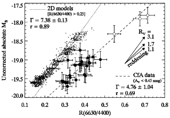
The models yield values for $\mathcal{R}(6630/4400)$ ranging between $\sim 0.12$ and $\sim 0.44$, all due to intrinsic color variations. Since these models reproduce the relation between $M_{B}$ and post-maximum decline rate of Phillips (1993), they confirm the intrinsic nature of the correlation between $\mathcal{R}(6630/4400)$ and $\{x_{1},c\}$ shown in Fig. 6 (upper left panel).

The wavelength bins $\lambda_{X}=6630$ Å and $\lambda_{Y}=4400$ Å are close to the central wavelengths of the standard $R$ and $B$ broadband filters, hence $\mathcal{R}(6630/4400)$ is a rough measure of the $B-R$ color at $B$-band maximum. The 2D models of Fig. 10 indicate that a large part of the variation in $\mathcal{R}(6630/4400)$ seen in the data is due to intrinsic variations in $B-R$ color. Reddening in the host galaxy is then needed to explain values of $\mathcal{R}(6630/4400)\gtrsim 0.4$, while at lower values it is challenging at best to discriminate between the effects of intrinsic color variations and extinction by dust, since both affect $\mathcal{R}(6630/4400)$ in the same manner, as illustrated by the reddening vectors in Fig. 10 [they are really reddening curves, cf. Fig. 3, but the behavior is almost linear over this small range in $\mathcal{R}(6630/4400)$].

The models also give a physical explanation for the correlation of $\mathcal{R}(6630/4400)$ with absolute magnitude. Indeed, the variation of this ratio is largely caused by spectroscopic variations around 4400 Å, a region dominated by lines of Fe II and Fe III, with contributions from Mg II (Ti II provides an important source of opacity for the least luminous SN Ia), while the region around 6630 Å has little intrinsic variation (this was noted by Bailey et al. 2009). This translates to a standard deviation of peak $B$-band magnitudes ($\sigma\approx 0.40$ mag) that is almost twice as large as the $R$-band magnitude (at $B$ maximum; $\sigma\approx 0.26$ mag) in the models. The relative contribution of Fe II and Fe III lines is related to the temperature of the line-forming regions in the SN Ia ejecta, itself a function of peak luminosity (dimmer SN Ia are generally cooler; see, e.g., Kasen & Woosley 2007). One thus expects a large luminosity-dependent spectroscopic variation in this wavelength region, although its exact shape and relation to temperature remains largely unknown.

While these models provide useful insights into the physical origin of these correlations, a direct comparison with the data reveals some of their shortcomings. In Fig. 10 we see that some models predict values of the flux ratio $\mathcal{R}(6630/4400)\lesssim 0.25$ for the most luminous SN Ia, where the data are limited to values greater than this. Our sample includes several SN Ia at the high luminosity end that show no sign of extinction in their host galaxies ($A_{V}<0.05$ mag based on light-curve fits with MLCS2k2), so the differences are real and point to discrepancies between the data and the models, some of the latter having bluer $B-R$ colors at $B$-band maximum. This is not surprising, as the models explore a larger range of parameter space than is realized in nature. Comparisons of this sort can then help constrain the range of model input parameters. A more detailed comparison of SN Ia data from the CfA SN program with these models will be presented elsewhere.

4.4 Results on spectra at other ages

Bailey et al. (2009) restricted their analysis to spectra within $\Delta t=2.5$ d from $B$-band maximum. In this section we consider flux ratios measured on spectra at other ages. We impose the same cuts on relative flux calibration accuracy ($|\Delta(B-V)|<0.1$ mag), SALT2 color ($c<0.5$), redshift ($z>0.015$), and age range ($\Delta t=2.5$ d) as those used for the maximum-light spectra in the previous section. We consider all ages between $t=-2.5$ d and $t=+7.5$ d, in steps of 2.5 d (for ages earlier than $-2.5$ d or later than +7.5 d the number of SN Ia with spectra that satisfy our cuts falls below 20, and we do not trust the results). We report the best ratio at each age in Table 4, for both the $\mathcal{R}$-only and $(c,\mathcal{R}^{c})$ models.

Table 4: Top flux ratio at ages $-2.5\leq t\leq+7.5$ d from 10-fold CV

Rank	$\lambda_{X}$	$\lambda_{Y}$	$\gamma$	WRMS	$\sigma_{\rm pred}$	$\rho_{x_{1},c}$	$\Delta_{x_{1},c}$	$N_{\rm SNIa}$
$\mathcal{R}$
$-2.5$	6540	4580	$-6.09\pm 0.11$	$0.182\pm 0.025$	$0.151\pm 0.031$	$0.70\pm 0.13$	$-0.032\pm 0.028\ (1.1\sigma)$	24
$+0.0$	6630	4400	$-4.37\pm 0.09$	$0.189\pm 0.026$	$0.163\pm 0.030$	$0.80\pm 0.09$	$-0.018\pm 0.025\ (0.7\sigma)$	26
$+2.5$	6630	4040	$-3.51\pm 0.09$	$0.203\pm 0.027$	$0.171\pm 0.033$	$0.63\pm 0.13$	$-0.012\pm 0.033\ (0.4\sigma)$	26
$+5.0$	6590	4490	$-4.69\pm 0.12$	$0.225\pm 0.031$	$0.203\pm 0.034$	$0.36\pm 0.20$	$0.022\pm 0.041\ (0.5\sigma)$	26
$+7.5$	6590	4890	$-3.40\pm 0.20$	$0.251\pm 0.035$	$0.229\pm 0.039$	$0.47\pm 0.18$	$0.044\pm 0.043\ (1.0\sigma)$	25
$(c,\mathcal{R}^{c})$
$-2.5$	4610	4260	$2.19\pm 0.14$	$0.143\pm 0.020$	$0.106\pm 0.028$	$0.43\pm 0.23$	$-0.081\pm 0.037\ (2.2\sigma)$	24
$+0.0$	6420	5290	$-1.75\pm 0.10$	$0.175\pm 0.025$	$0.148\pm 0.029$	$0.80\pm 0.09$	$-0.032\pm 0.023\ (1.4\sigma)$	26
$+2.5$	5550	6630	$1.09\pm 0.08$	$0.169\pm 0.022$	$0.133\pm 0.030$	$0.79\pm 0.09$	$-0.049\pm 0.027\ (1.8\sigma)$	26
$+5.0$	6540	5580	$-5.18\pm 0.48$	$0.194\pm 0.026$	$0.166\pm 0.031$	$0.57\pm 0.16$	$-0.014\pm 0.034\ (0.4\sigma)$	26
$+7.5$	6460	5510	$-1.85\pm 0.13$	$0.200\pm 0.028$	$0.173\pm 0.033$	$0.79\pm 0.09$	$-0.007\pm 0.027\ (0.3\sigma)$	25

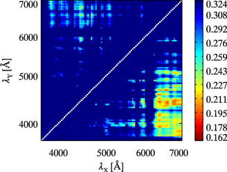
The 2D maps of Hubble diagram residual scatter for spectra at ages $t=-2.5$, +0, +5, and +7.5 d are shown in Fig. 11. As was the case for maximum-light spectra, adding the SALT2 $x_{1}$ parameter leads to slightly degraded results when compared with $\mathcal{R}$ alone, so we do not show plots for $(x_{1},\mathcal{R})$ in Fig. 11. Moreover, we do not show results for $(x_{1},c,\mathcal{R}^{c})$ since the best color-corrected flux ratios in this case do not result in a significant improvement over $(c,\mathcal{R}^{c})$. At all the ages we consider here, the set of predictors $(c,\mathcal{R}^{c})$ results in lower weighted rms of prediction residuals than $(x_{1},c)$, although the significance of the difference is $\lesssim 2\sigma$ and is lower for $t\geq+5$ d than for $-2.5\leq t\leq+2.5$ d. A flux ratio by itself only leads to an improvement over $(x_{1},c)$ near maximum light ($-2.5\leq t\leq+2.5$ d). As was the case at maximum light, there is a positive intrinsic correlation in prediction error between all the distance prediction models that include a flux ratio and $(x_{1},c)$ [$0.4\lesssim\rho_{x_{1},c}\lesssim 0.8$].

	WRMS$(\mathcal{R})$   [mag]	WRMS$(c,\mathcal{R}^{c})$   [mag]
$t=-2.5$ d
$t=+0$ d
$t=+5$ d
$t=+7.5$ d

Figure 11: Results from 10-fold cross-validation on spectra at $t=-2.5,+0,+5,+7.5$ d. (from top to bottom), color-coded according to the weighted rms of prediction Hubble residuals. The left column is corresponds to $\mathcal{R}$ only, while the right column corresponds to the $(c,\mathcal{R}^{c})$ model.

The best set of predictors overall in the age range $-2.5\leq t\leq+7.5$ d is $[c,\mathcal{R}^{c}(4610/4260)]$ at $t=-2.5$ d. The weighted rms of prediction residuals is reduced by $\sim 30$% with respect to $(x_{1},c)$ [${\rm WRMS}=0.143\pm 0.020$ mag], and the intrinsic prediction error by $\sim 40$% ($\sigma_{\rm pred}=0.106\pm 0.028$ mag), the significance of the difference being $\sim 2\sigma$ ($\Delta_{x_{1},c}=-0.081\pm 0.037$ mag). We show the correlation of $\mathcal{R}^{c}(4610/4260)$ at $t=-2.5$ d and the SALT2 parameters $(x_{1},c)$ in Fig. 12. This color-corrected ratio is mildly correlated with $x_{1}$ [$r=0.61$; this drops slightly to $r=0.47$ if we ignore the two points at $\mathcal{R}^{c}(4610/4260)>1.3$] and uncorrelated with color ($r=-0.40$; this drops to $r=0.03$ if we ignore the two points at $c>0.4$). Interestingly, the wavelength bins that constitute this ratio are part of the two prominent spectral absorption features, predominantly due to iron-group elements, that were found to vary intrinsically between SN Ia based on the 2D models discussed in § 4.3.4.

Figure 12: Correlation between $\mathcal{R}^{c}(4610/4260)$ at $t=-2.5$ d and the SALT2 fit parameters $(x_{1},c)$. The Pearson coefficient of the correlation with color drops to $r=0.03$ if we ignore the two points at $c>0.4$.

4.5 Results using two flux ratios

In this section we consider corrections using a linear combination of two flux ratios as follows:

$$\mu = m_{B}-M+\gamma_{1}\mathcal{R}_{1}+\gamma_{2}\mathcal{R}_{2}$$ (14)

$$\mu = m_{B}-M-\beta c+\gamma_{1}\mathcal{R}_{1}^{c}+\gamma_{2}\mathcal{R}_{2}^{c},$$ (15)

where the latter equation includes an additional correction due to color, hence the use of color-corrected ratios $\mathcal{R}^{c}$. For both cases, we fix $\mathcal{R}_{1}^{(c)}$ to the highest-ranked single flux ratio [e.g., at maximum light: $\mathcal{R}_{1}(6630/4400)$ and $\mathcal{R}_{1}^{c}(6420/5290)$; see Table 2], but leave both $(\gamma_{1},\gamma_{2})$ as free parameters (i.e. we do not set $\gamma_{1}$ equal to $\gamma$ found in the single flux ratio case).

The results for the top five secondary flux ratios at maximum light are displayed in Table 5. In all cases, including a second flux ratio further reduces the weighted rms of prediction residuals by $\approx$15-20% [${\rm WRMS}=0.162\pm 0.022$ mag for $\mathcal{R}_{2}(5160/5290)$; ${\rm WRMS}=0.151\pm 0.021$ mag for $\mathcal{R}_{2}^{c}(5690/5550)$] with respect to the single flux ratio case [${\rm WRMS}=0.189\pm 0.026$ mag for $\mathcal{R}(6630/4400)$; ${\rm WRMS}=0.175\pm 0.025$ mag for $\mathcal{R}^{c}(6420/5290)$]. Again the significance of the improvement ($\lesssim 2\sigma$) is difficult to gauge given our sample size, this despite the fact that $\gamma_{2}$ is significantly different from zero in all cases. Our best secondary flux ratios, $\mathcal{R}_{2}(5160/5290)$ and $\mathcal{R}^{c}_{2}(5690/5550)$, are uncorrelated with the SALT2 fit parameters $(x_{1},c)$ and with the highest-ranked primary ratios $\mathcal{R}_{1}(6630/4400)$ and $\mathcal{R}^{c}_{1}(6420/5290)$ [see Fig. 13], and hence provide independent information on SN Ia luminosity.

Table 5: Top 5 secondary flux ratios at maximum light from 10-fold CV on 26 SN Ia

Rank	$\lambda_{X}$	$\lambda_{Y}$	$\gamma_{1}$	$\gamma_{2}$	WRMS	$\sigma_{\rm pred}$	$\rho_{x_{1},c}$	$\Delta_{x_{1},c}$
$[\mathcal{R}_{1}(6630/4400),\mathcal{R}_{2}]$
1	5160	5290	$-5.05\pm 0.17$	$-2.24\pm 0.22$	$0.162\pm 0.022$	$0.127\pm 0.028$	$0.32\pm 0.23$	$-0.052\pm 0.038\ (1.4\sigma)$
2	5290	5160	$-5.08\pm 0.18$	$4.78\pm 0.50$	$0.167\pm 0.022$	$0.133\pm 0.029$	$0.31\pm 0.24$	$-0.046\pm 0.036\ (1.3\sigma)$
3	5120	5290	$-5.19\pm 0.11$	$-1.75\pm 0.20$	$0.172\pm 0.024$	$0.141\pm 0.029$	$0.41\pm 0.21$	$-0.038\pm 0.036\ (1.1\sigma)$
4	5690	5360	$-3.93\pm 0.12$	$-2.06\pm 0.21$	$0.172\pm 0.024$	$0.141\pm 0.029$	$0.46\pm 0.20$	$-0.038\pm 0.032\ (1.2\sigma)$
5	5690	5290	$-4.14\pm 0.11$	$-1.26\pm 0.13$	$0.172\pm 0.024$	$0.142\pm 0.029$	$0.48\pm 0.19$	$-0.038\pm 0.032\ (1.2\sigma)$
$[c,\mathcal{R}_{1}^{c}(6420/5290),\mathcal{R}_{2}^{c}]$
1	5690	5550	$-1.69\pm 0.09$	$-1.93\pm 0.21$	$0.151\pm 0.021$	$0.115\pm 0.027$	$0.58\pm 0.17$	$-0.063\pm 0.030\ (2.1\sigma)$
2	5690	5960	$-2.34\pm 0.11$	$-1.90\pm 0.23$	$0.152\pm 0.020$	$0.116\pm 0.028$	$0.42\pm 0.21$	$-0.064\pm 0.035\ (1.8\sigma)$
3	5960	5690	$-2.35\pm 0.11$	$2.05\pm 0.24$	$0.153\pm 0.021$	$0.117\pm 0.028$	$0.43\pm 0.21$	$-0.063\pm 0.036\ (1.8\sigma)$
4	5550	5690	$-1.70\pm 0.09$	$1.72\pm 0.20$	$0.152\pm 0.021$	$0.118\pm 0.027$	$0.58\pm 0.17$	$-0.061\pm 0.031\ (2.0\sigma)$
5	4890	5690	$-1.25\pm 0.10$	$1.22\pm 0.24$	$0.158\pm 0.021$	$0.122\pm 0.028$	$0.62\pm 0.15$	$-0.052\pm 0.026\ (2.0\sigma)$

Figure 13: Correlation between the highest-ranked $(\mathcal{R}_{2},\mathcal{R}^{c}_{2})$ at maximum light and the SALT2 fit parameters $(x_{1},c)$, and the highest-ranked $(\mathcal{R}_{1},\mathcal{R}^{c}_{1})$.

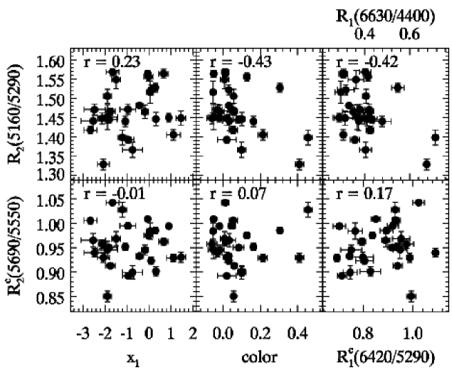
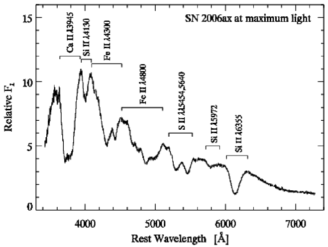
The secondary flux ratios $\mathcal{R}_{2}$ listed in Table 5 have a much smaller wavelength baseline than the primary ratios $\mathcal{R}_{1}$ and $\mathcal{R}^{c}_{1}$ (see Table 2). The highest-ranked secondary ratios have a 130 Å and 140 Å baseline, respectively. These ratios do not measure SN Ia colors: they measure small-scale intrinsic spectroscopic variations. Interestingly, all the wavelength bins that form these secondary ratios are clustered around the S II $\lambda$$\lambda$5454,5640 doublet and the iron-group-dominated absorption complex Fe II $\lambda$4800 mentioned in § 4.4 (see also § 4.3.4). As was the case for a single flux ratio, the results using a secondary flux ratio are similar for $-2.5\leq t\leq+2.5$ d, and tend to be worse at later ages. We choose not to discuss them further.

In a recent paper, Yu et al. (2009) have searched for flux ratio pairs that minimize Hubble diagram residuals (with no color correction), and find several such pairs which achieve a standard deviation $\sigma\lesssim 0.10$ mag at ages between $-3$ d and +12 d from maximum light. We have validated the flux ratio pairs reported in their Table 4 and find that none of them lead to an improvement compared with the standard $(x_{1},c)$ model. There could be several reasons for this disagreement: Yu et al. (2009) do not use a cross-validation procedure and their sample size (anywhere between 17 and 24 SN Ia depending on the age and flux ratio pair considered) suggests they may be overfitting a small sample. Moreover, they use color-corrected flux ratios (actually corrected for the host-galaxy extinction, $A_{V}$, as opposed to the SALT2 color parameter) but do not include a color parameter in their equation to correct for the SN Ia magnitudes. When we use the SALT2 color parameter in addition to the same flux ratio pairs as Yu et al. (2009), several pairs indeed lead to an improvement over the standard $(x_{1},c)$ model, but not over the correction using a single flux ratio (or a single flux ratio in combination with color) we find in this paper. Last, Yu et al. (2009) do not impose a redshift cut on their sample: only 14 out of 38 SN Ia are at redshifts $z>0.015$, and 5 are at redshifts $z<0.005$, where the magnitude error due to peculiar velocities is $\sigma_{\rm pec}>0.4$ mag. It is unclear why this should lead to a lower scatter in Hubble residuals (on the contrary one expects an increased scatter), but it certainly impacts their analysis.

5 Other spectroscopic indicators

In this section we consider other spectroscopic indicators, mostly related to spectral line profile morphology. Some of these indicators are also flux ratios, but the wavelengths correspond to precise locations of absorption troughs or emission peaks in the SN Ia spectrum, as opposed to the “blind” approach of computing flux ratios from all possible wavelength bins with no a priori physical motivation. We use the same approach as for the flux ratios, i.e. we consider models for predicting SN Ia distances which include a spectroscopic indicator, possibly in combination with a light-curve parameter (cf. Eq. 1), and we validate each model using $K$-fold cross-validation (and present results for $K=10$ in this section).

5.1 Measurements

We divide the SN Ia spectrum into several “features”, each labeled according to the strongest line in that wavelength range. Figure 14 shows the seven features we consider in this paper, from Ca II $\lambda$3945 in the blue to Si II $\lambda$6355 in the red. The wavelengths associated with each feature correspond to the $gf$-weighted mean wavelength of the different atomic transitions for the specified ion (e.g. 3945 Å for the Ca II H & K lines), except for the two large features dominated by Fe II lines, where the wavelengths denote the approximate location of the deepest absorption ($\sim 4300$ Å and $\sim 4800$ Å). The Fe II $\lambda$4300 feature also includes contributions from Mg II, and possibly Fe III for the most luminous SN Ia. For the faintest, 1991bg-like SN Ia, Ti II constitutes a dominating source of opacity in this wavelength region. Since we do not include 1991bg-like SN Ia in our analysis, however, we do not present measurements for Ti II.

Figure 14: Wavelength bounds of spectroscopic features for which we measured the various indicators shown in Fig. 15, illustrated using the maximum-light spectrum of SN 2006ax.

The various spectroscopic indicators we consider are illustrated in Fig. 15, based on the Si II $\lambda$6355 line profile in the spectrum of SN 2005ki at $t=+1$ d from maximum light. We first smooth the spectrum using the inverse-variance Gaussian filter of Blondin et al. (2006) with a smoothing factor $0.001<d\lambda/\lambda<0.01$ determined based on a $\chi^{2}$ test using flux errors from the variance spectra (Fig. 15; thick line). The smoothed spectrum makes it easier to define wavelength locations of local flux maxima on either side of the absorption component of the P Cygni profile ($\lambda_{\rm blue}$ and $\lambda_{\rm peak}$), as well as the location of maximum absorption ($\lambda_{\rm abs}$). The wavelengths $\lambda_{\rm abs}$ and $\lambda_{\rm peak}$ are then used to define the absorption and peak velocities, respectively ($v_{\rm abs}$ and $v_{\rm peak}$), using the relativistic Doppler formula (see also Blondin et al. 2006). We also measure the heights of the local maximum ($h_{\rm blue}$ and $h_{\rm peak}$), and define a pseudo-continuum between them. These latter quantities are measured on the original, unsmoothed spectrum. Division by this pseudo-continuum enables us to measure the relative absorption depth ($d_{\rm abs}$) and full-width at half-maximum (FWHM) of the absorption component, as well as its pseudo-equivalent width (pEW; defined analogously to the equivalent width used by stellar spectroscopists for abundance determinations, but without the physical basis, hence “pseudo” EW; Fig. 15; right panel).

Figure 15: Definition of the main spectroscopic indicators used in this paper, here illustrated using the Si II $\lambda$6355 line profile in the spectrum of SN 2005ki at $t=+1$ d. The right panel shows the pseudo-continuum (dashed line), as well as the wavelength locations of the blue and red emission peaks ($\lambda_{\rm blue}$ and $\lambda_{\rm peak}$) and their respective heights ($h_{\rm blue}$ and $h_{\rm peak}$). The wavelength of maximum absorption ($\lambda_{\rm abs}$) serves to define the absorption velocity, $v_{\rm abs}$. The peak velocity $v_{\rm peak}$ is defined analogously. The left panel shows the same line profile normalized to the pseudo-continuum, and serves to define the (relative) absorption depth ($d_{\rm abs}$), FWHM, and pseudo-equivalent width (pEW; shaded gray region). In both panels, the thick line corresponds to the smoothed flux, where we have used the inverse-variance weighted Gaussian filter of Blondin et al. (2006) with a smoothing factor $d\lambda/\lambda=0.005$.

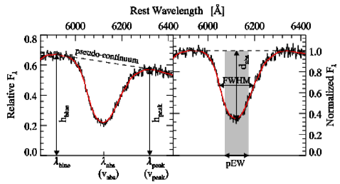
We measure these quantities for all the features presented in Fig. 14, except for the complex Fe II $\lambda$4300 and Fe II $\lambda$4800 features for which we only consider the pseudo-equivalent width. The error on each measured quantity includes errors due to redshift, relative flux calibration, host-galaxy extinction and contamination, and of course the flux error. We only consider measurements for which the mean S/N over the entire feature is greater than 5 per Å, and require a minimum of 20 SN Ia with valid measurements. Note that we do not impose cuts on relative flux calibration accuracy or SALT2 color, as was the case for the flux ratios, since these quantities are mostly local measurements which are far less sensitive to the overall SED.

We also consider various spectroscopic ratios, which were found to correlate with absolute magnitude, defined below:

$$\mathcal{R}(\rm Ca) = \frac{h_{\rm peak}(\rm Ca\,{\sc II}\,\lambda 3945)}{h_{\rm blue}(\rm Ca\,{\sc II}\,\lambda 3945)}$$ (16)

$$\mathcal{R}(\rm CaS) = \frac{\int_{3887}^{4012}F_{\lambda}d\lambda}{\int_{3620}^{3716}F_{\lambda}d\lambda}$$ (17)

$$\mathcal{R}(\rm Si) = \frac{d_{\rm abs}(\rm Si\,{\sc II}\,\lambda 5972)}{d_{\rm abs}(\rm Si\,{\sc II}\,\lambda 6355)}$$ (18)

$$\mathcal{R}(\rm SiS) = \frac{h_{\rm peak}(\rm Si\,{\sc II}\,\lambda 6355)}{h_{\rm peak}(\rm S\,{\sc II}\,\lambda 5640)}$$ (19)

$$\mathcal{R}(\rm SiSS) = \frac{\int_{5500}^{5700}F_{\lambda}d\lambda}{\int_{6200}^{6450}F_{\lambda}d\lambda}$$ (20)

$$\mathcal{R}(\rm S,Si) = \frac{\rm pEW(S\,{\sc II}\,\lambda\lambda 5454,5640)}{\rm pEW(Si\,{\sc II}\,\lambda 5972)}$$ (21)

$$\mathcal{R}(\rm Si,Fe) = \frac{\rm pEW(Si\,{\sc II}\,\lambda 5972)}{\rm pEW(Fe\,{\sc II}\,\lambda 4800)}.$$ (22)

The ratios $\mathcal{R}(\rm Ca)$ and $\mathcal{R}(\rm Si)$ were both defined by Nugent et al. (1995), and found to correlate well with the luminosity decline rate parameter $\Delta m_{15}(B)$. To increase the S/N of the $\mathcal{R}(\rm Ca)$ measurement, Bongard et al. (2006) introduced the corresponding integral flux ratio $\mathcal{R}(\rm CaS)$, also found to correlate with absolute magnitude. Using a grid of LTE synthetic spectra to investigate the $\mathcal{R}(\rm Si)$ wavelength region, Bongard et al. (2006) also defined a ratio of the red local maximum of Si II $\lambda$6355 to the red local maximum of S II $\lambda$5640, noted $\mathcal{R}(\rm SiS)$. The corresponding integral flux ratio is $\mathcal{R}(\rm SiSS)$, again introduced by Bongard et al. (2006) to increase the S/N of the $\mathcal{R}(\rm SiS)$ measurement. Last, Hachinger et al. (2006) measured the absorption velocities and pseudo-EW in 28 SN Ia spectra and found two additional pEW ratios, $\mathcal{R}(\rm S,Si)$ and $\mathcal{R}(\rm Si,Fe)$, that are good indicators of luminosity. Note that $\mathcal{R}(\rm Ca)$ and $\mathcal{R}(\rm SiS)$ are in fact flux ratios similar to those defined by Bailey et al. (2009).

5.2 Results

We present our results using the absorption velocity ($v_{\rm abs}$; units of $10^{4}$   km  s^-1), the full-width at half-maximum (FWHM; units of $10^{2}$ Å), the relative absorption depth ($d_{\rm abs}$), the pseudo-equivalent width (pEW; units of $10^{2}$ Å), and the various spectroscopic ratios $\mathcal{R}(X)$ [Eqs. 16-22] in Tables 6-10 (Appendix C). We do not present results for the peak velocity ($v_{\rm peak}$) as they are far worse than for the other indicators. There were not enough valid measurements for Ca II $\lambda$3945, hence the absence of this line in Tables 6-9. We only report results for the bluer absorption of the S II doublet (S II $\lambda$5454) in Tables 6-8, but the pseudo-equivalent width is that of the entire doublet (see Table 9).

Based on the difference in intrinsic prediction error with respect to the standard model which uses the SALT2 fit parameters $(x_{1},c)$, again noted $\Delta_{x_{1},c}$, we see from Tables 6-10 that none of these spectroscopic indicators alone leads to a lower weighted rms of prediction residuals (i.e. $\Delta_{x_{1},c}>0$). At best they are consistent with no improvement at all [e.g. pEW(Si II $\lambda$4130), for which $\Delta_{x_{1},c}=0.041\pm 0.033$ mag)]. The same is true at ages other than maximum light.

Nonetheless, several such indicators compete well with $(x_{1},c)$, even leading to small improvements (albeit statistically insignificant), but only when combined with SALT2 color [pEW(Si II $\lambda$4130) and $\mathcal{R}$(Si)] or in addition to $(x_{1},c)$ [$v_{\rm abs}$(Si II $\lambda$6355 and $d_{\rm abs}$(S II $\lambda$5454)]. We discuss these indicators in the two following sections.

5.2.1 Spectroscopic indicators in combination with SALT2 color

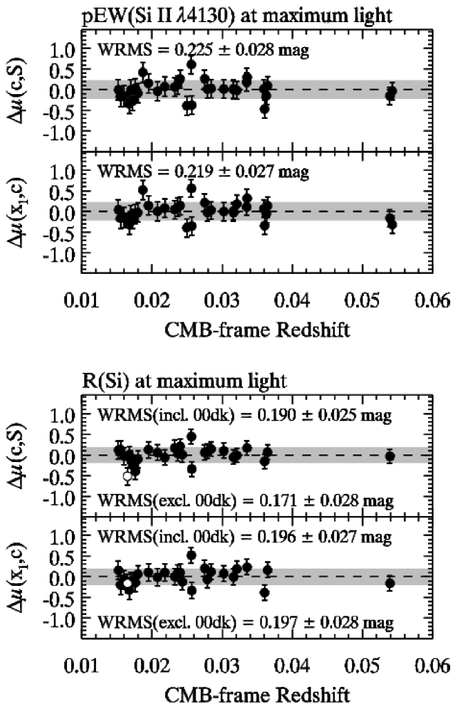
When used in combination with the SALT2 color parameter, both the pseudo-equivalent width of Si II $\lambda$4130 and the $\mathcal{R}$(Si) spectroscopic ratio compete well with the standard $(x_{1},c)$ predictors ($\Delta_{x_{1},c}=0.006\pm 0.014$ mag and $\Delta_{x_{1},c}=-0.007\pm 0.030$ mag). Both indicators are strongly anti-correlated with $x_{1}$ and uncorrelated with SALT2 color (see Fig. 16, left and middle panels), while the correlation with color-corrected Hubble residual is more pronounced for $\mathcal{R}$(Si) [$r=0.63$] than for pEW(Si II $\lambda$4130) [$r=0.35$]. In a sense, both indicators act to replace the light-curve width parameter $x_{1}$. The anti-correlation of $\mathcal{R}$(Si) with $x_{1}$ has been recovered by several authors since its publication by Nugent et al. (1995), while the relation between pEW(Si II $\lambda$4130) and light-curve shape has more recently been mentioned by Arsenijevic et al. (2008) and Walker et al. (2010).

Figure 16: Correlation between pEW(Si II $\lambda$4130) and $\mathcal{R}({\rm Si})$ at maximum light and the SALT2 fit parameters $(x_{1},c)$, and color-corrected Hubble residual. The open circle in the lower panels corresponds to SN 2000dk.

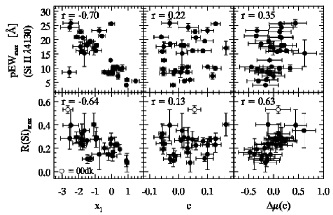
We show the Hubble residuals obtained when using pEW(Si II $\lambda$4130) and $\mathcal{R}$(Si) in combination with SALT2 color in Fig. 17, where we also show the residuals from the standard $(x_{1},c)$ model. The subluminous (but not 1991bg-like) SN 2000dk stands out as a $\lesssim 2\sigma$ outlier for $[c,\mathcal{R}$(Si)], while this is not the case for $(x_{1},c)$ [the point corresponding to SN 2000dk is highlighted in both Figs. 16 and 17]. This single SN contributes a large fraction of the residual scatter [${\rm WRMS\ (incl.00dk)}=0.190\pm 0.025$ mag cf. $0.196\pm 0.027$ mag for $(x_{1},c)$], and excluding it from the sample leads to a $\sim 10\%$ decrease in the weighted rms of prediction Hubble residuals, resulting in a $\sim 15$% improvement over $(x_{1},c)$ [${\rm WRMS\ (excl.00dk)}=0.171\pm 0.028$ mag cf. $0.197\pm 0.028$ mag for $(x_{1},c)$].

Figure 17: Hubble diagram residuals for pEW(Si II $\lambda$4130) [top] and $\mathcal{R}({\rm Si})$ [bottom] at maximum light. In each case we show the Hubble residuals obtained using SALT2 color and the spectroscopic indicator (upper panels), and using the standard SALT2 fit parameters $(x_{1},c)$ (lower panels). We also indicate the weighted rms of Hubble residuals (gray highlighted region). For the $\mathcal{R}({\rm Si})$ spectroscopic indicator, we report the weighted rms both including and excluding SN 2000dk (open circle).

5.2.2 Spectroscopic indicators in addition to the SALT2 fit parameters $(x_{1},c)$

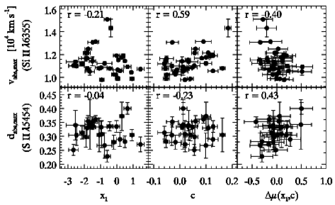
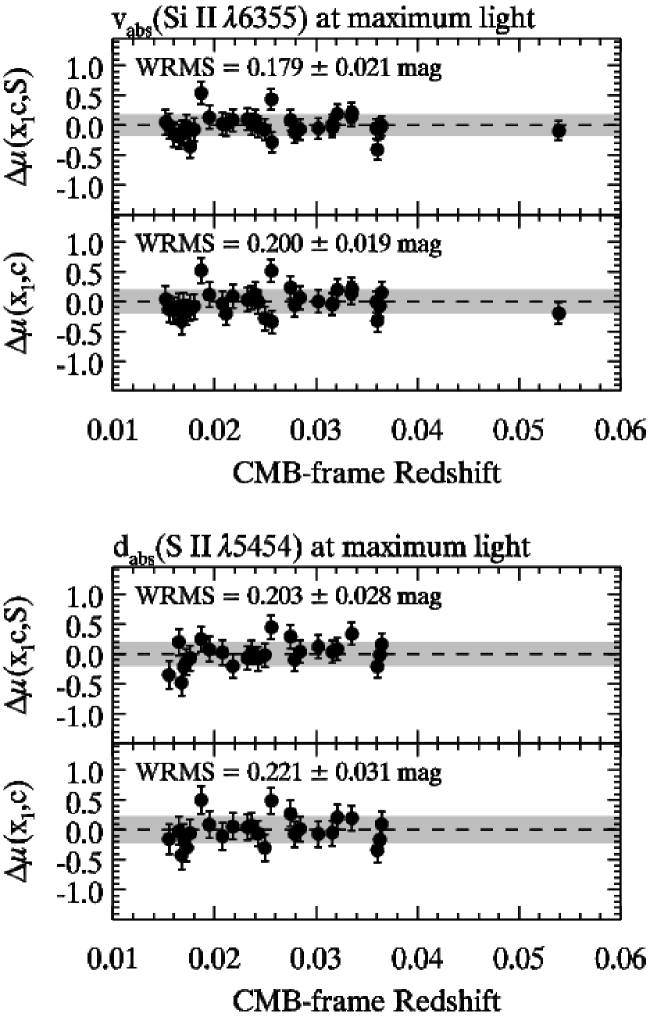
When used in addition to the standard SALT2 fit parameters $(x_{1},c)$, both the absorption velocity of Si II $\lambda$6355 and the relative absorption depth of S II $\lambda$5454 result in a $\lesssim 10$% decrease in the weighted rms of prediction residuals ($\Delta_{x_{1},c}=-0.020\pm 0.019$ mag and $\Delta_{x_{1},c}=-0.022\pm 0.030$ mag), although the apparent improvement for $d_{\rm abs}$(S II $\lambda$5454) is due to the fact that the weighted rms of prediction residuals for the $(x_{1},c)$ model is somewhat larger for this particular sample (${\rm WRMS}=0.221\pm 0.031$ mag). Both these spectroscopic indicators are uncorrelated with $x_{1}$ or color [Fig. 18; the apparent correlation of $v_{\rm abs}$(Si II $\lambda$6355) with color ($r=0.59$) is destroyed if we ignore the one point at $c\approx 0.2$], and thus provide additional information independent of light-curve shape or color. The correlation with $(x_{1},c)$-corrected Hubble residuals (Fig. 18, right panels) is only modest ($|r|\approx 0.40$ for both indicators), and should be reviewed as more data become publicly available.

Figure 18: Correlation between $v_{\rm abs}$(Si II $\lambda$6355) and $d_{\rm abs}$(S II $\lambda$5454) at maximum light and the SALT2 fit parameters $(x_{1},c)$, and $(x_{1},c)$-corrected Hubble residual.

We show the Hubble residuals obtained when using $v_{\rm abs}$(Si II $\lambda$6355) and $d_{\rm abs}$(S II $\lambda$5454) in addition to the standard $(x_{1},c)$ predictors in Fig. 19. One clearly sees from these diagrams that the impact of the additional spectroscopic indicator is fairly small, as the sign and magnitude of the residuals are almost the same for $(x_{1},c,\mathcal{S})$ and $(x_{1},c)$. This is further confirmed by looking up the value for the intrinsic correlation in prediction error for both indicators in Tables 6 and 8: $\rho_{x_{1},c}=0.83\pm 0.06$ for $v_{\rm abs}$(Si II $\lambda$6355) and $\rho_{x_{1},c}=0.75\pm 0.10$ for $d_{\rm abs}$(S II $\lambda$5454).

Figure 19: Hubble diagram residuals for $v_{\rm abs}$(Si II $\lambda$6355) [top], and $d_{\rm abs}$(S II $\lambda$5454) [bottom] at maximum light. In each case we show the Hubble residuals obtained using the spectroscopic indicator in addition to the SALT2 fit parameters $(x_{1},c)$ (upper panels), and using $(x_{1},c)$ only (lower panels). We also indicate the weighted rms of Hubble residuals (gray highlighted region).

5.2.3 Results using multiple indicators

We have also considered models involving a linear combination of two spectroscopic indicators (i.e. $\mu=m_{B}-M+\gamma_{1}\mathcal{S}_{1}+\gamma_{2}\mathcal{S}_{2}$) or a ratio of two indicators (i.e. $\mu=m_{B}-M+\gamma\mathcal{S}_{1}/\mathcal{S}_{2}$), also for cases including the SALT2 fit parameters $(x_{1},c)$. No combination of two of these spectroscopic indicators leads to an improvement over the single indicator case, regardless of the age considered.

6 Discussion: do SN Ia spectra really help?

The central question this paper addresses is whether spectra yield useful information to predict distances to SN Ia better than light-curve width and color alone. The answer to this question can have a significant impact on the way future SN Ia surveys are planned, namely whether or not they should include spectroscopic (or spectro-photometric) capabilities. This has been (and remains!) an active area of discussion for proposals for space-borne missions within the framework of the Dark Energy Task Force (Albrecht et al. 2009) or the US Astronomy & Astrophysics Decadal Survey.

Of all the spectroscopic indicators considered in this paper, the concept of flux ratio introduced by Bailey et al. (2009) appears to be the most promising, yielding up to $\sim 30\%$ lower Hubble residual scatter than when using the standard light-curve parameters. However, given the limited sizes of the SN-Factory (58 SN Ia) and CfA (26 SN Ia) samples on which the method has been applied, the results are at best statistically significant at the $\lesssim 2\sigma$ level, and the method should be validated on much larger samples. It should be noted that the measurement of flux ratios requires accurate relative flux calibration, as well as minimal contamination by host-galaxy light. Both requirements impose strong conditions on future SN Ia surveys that plan to use this method.

The other spectroscopic indicators we consider in this paper are intimately linked to line-profile shapes of specific SN Ia spectral features. One would have hoped that such a physically-motivated approach would yield interesting results, but this is not the case. At best, these indicators yield $\lesssim 1\sigma$ lower residual scatter compared with the standard light-curve parameters. This is rather disappointing, but also points to potential problems with the measurement method we use. It is largely automated, but requires some human interaction to ensure the correct local maxima used to define the wavelength bounds of each feature are selected. Moreover, while some indicators (such as the absorption velocity $v_{\rm abs}$) are largely insensitive to host-galaxy reddening, others (such as the pseudo-EW) are strongly affected. Recent unbiased techniques based on wavelet transforms have been proposed that are largely insensitive to these measurement issues (Wagers et al. 2010), and the present analysis could be repeated with such techniques.

Last, given our spectroscopic data we have focused exclusively on the optical region, but there appears to be spectroscopic indicators that correlate with luminosity in other wavelength regions (UV: Foley et al. 2008; NIR: Marion et al., in preparation). An increased spectroscopic sample at these wavelengths might reveal spectroscopic quantities that lead to even more precise distances to SN Ia than optical flux ratios.

7 Conclusions

We have investigated the use of spectroscopic indicators which, when used alone or in conjunction with light-curve parameters (width and color), predict distances to SN Ia better than when using the standard combination of light-curve width and color. We have carried our a $K$-fold cross-validation analysis on a large spectroscopic data set obtained through the CfA Supernova Program. We constructed and implemented maximum likelihood estimators for the rms intrinsic prediction error of a given method, and the intrinsic covariance of prediction errors of different methods. We used these estimates to compare predictive models for SN Ia distances in a quantitative manner.

We first considered the spectroscopic flux ratios of Bailey et al. (2009), highlighting the importance of an accurate relative flux calibration and the failure of this method for highly-reddened objects (SALT2 color $c>0.5$). At maximum light, our best single flux ratio $\mathcal{R}(6630/4400)$ from 26 SN Ia at $z>0.015$ leads to a $\sim 10$% lower weighted rms of cross-validated prediction Hubble residuals (${\rm WRMS}=0.189\pm 0.026$ mag) than when using the standard SALT2 light-curve width ($x_{1}$) and color ($c$) parameters (${\rm WRMS}=0.204\pm 0.029$ mag), at 0.7$\sigma$ significance. When used in combination with the SALT2 color parameter, our best color-corrected flux ratio $\mathcal{R}^{c}(6420/5290)$ leads to $\sim 15$% lower weighted rms (${\rm WRMS}=0.175\pm 0.025$ mag), at 1.4$\sigma$ significance. We thus confirm the use of flux ratios in improving distance measurements of SN Ia magnitudes, although the significance of the difference with respect to the standard purely photometric approach is difficult to gauge given our sample size. We also point to differences between the best ratios found in this paper and those reported by Bailey et al. (2009), in part due to the way these ratios are selected: Bailey et al. (2009) select their best ratios based on cross-correlation coefficients with uncorrected magnitudes, while we directly select them using the rms intrinsic error of cross-validated distance predictions in the Hubble diagram.

Comparison of our results with synthetic spectra from a 2D survey of delayed-detonation explosion models of Kasen et al. (2009) shows that a large part of the variation in our best single flux ratio $\mathcal{R}(6630/4400)$ is intrinsic and not due to reddening by dust. The correlation of this ratio with SN Ia magnitudes is due to the luminosity-dependent spectroscopic variation in the iron-group dominated absorption features around $\sim 4300$ Å. While the models confirm the presence of many flux ratios that correlate strongly with absolute magnitude, significant deviations exist with respect to the data. Such deviations can in principle be exploited to impose strong constraints on SN Ia models.

We extended the analysis of flux ratios to SN Ia spectra at other ages ($-2.5\leq t\leq+7.5$ d from maximum light (see Table 4). The best set of predictors overall in this age range is the color-corrected $\mathcal{R}^{c}(4610/4260)$ at $t=-2.5$ d combined with SALT2 color, which leads to $\sim 30$% lower weighted rms of prediction Hubble residuals with respect to $(x_{1},c)$ [${\rm WRMS}=0.143\pm 0.020$ mag], and to $\sim 40$% lower intrinsic prediction error ($\sigma_{\rm pred}=0.106\pm 0.028$ mag), at $\sim 2\sigma$ significance. The wavelength bins that constitute this ratio are part of the two prominent spectral absorption features predominantly due to iron-group elements, labeled Fe II $\lambda$4300 and Fe II $\lambda$4800, and which were found to vary intrinsically between SN Ia based on 2D models. Flux ratios at $t\geq+5$ d fare worse than at maximum light.

We also considered distance predictions based on two flux ratios. We find that the improvement over the standard ($x_{1},c$) model is at the $\lesssim 2\sigma$ level at best, and tends to be worse for ages $t\geq+5$ d. At maximum light, our best secondary ratios are $\mathcal{R}_{2}(5160/5290)$ and $\mathcal{R}^{c}_{2}(5690/5550)$, whose wavelength bins are clustered around the S II $\lambda$$\lambda$5454,5640 doublet and the iron-group-dominated absorption complex Fe II $\lambda$4800. Both ratios measure intrinsic small-scale differences between SN Ia that are uncorrelated with light-curve shape or color, and thus provide independent information on their luminosity.

We also considered spectroscopic indicators associated with spectral line-profile morphology: the absorption (and peak) velocity, the full-width at half maximum, the relative absorption depth, the pseudo-equivalent width, as well as other spectroscopic ratios. None of these spectroscopic indicators alone leads to a lower weighted rms of prediction Hubble residuals. Only when they are combined with SALT2 color do several indicators compete well with the standard predictors. Such is the case of the Si II $\lambda$4130 pseudo-EW and spectroscopic ratio $\mathcal{R}$(Si). Both indicators are correlated with $x_{1}$ and act as a replacement to light-curve shape in the distance prediction. When used in addition to $(x_{1},c)$, the Si II $\lambda$6355 absorption velocity and S II $\lambda$5454 relative absorption depth lead to a small improvement, albeit statistically insignificant. Using a linear combination of two such spectroscopic indicators and ratios thereof leads to no further improvement, whether at maximum light or at other ages.

Do spectra improve distance measurements of SN Ia? Yes, but not as much as we had hoped. The statistical framework developed here should be applied to an independent and larger sample to find out whether the effort of obtaining spectra for a cosmological sample will be repaid with better knowledge of dark energy.

Appendix A Sampling variance of weighted mean square error

If we assume the prediction errors are distributed normally with total variance, Eq. 5: $\Delta\mu_{s}\sim N(0,\sigma_{s}^{2})$, then the sampling variance of the weighted mean square error is

$$\text{Var}[\text{WRMS}^{2}]=\frac{2}{\left(\sum_{s=1}^{N}w_{s}\right)^{2}}\sum_{s=1}^{N}w_{s}^{2}\sigma_{s}^{4}.$$ (23)

The standard error on WRMS is then $\sqrt{\text{Var}[{\rm WRMS}^{2}]}/(2\times{\rm WRMS})$.

Appendix B Maximum likelihood estimators for intrinsic prediction error and covariance

Let the intrinsic variance of predictions ($\sigma_{\rm pred}^{2}$) from method $P,Q$ be $\sigma^{2}_{P},\sigma^{2}_{Q}$. Denote the intrinsic covariance between distance prediction errors from $P$ and $Q$ as $c_{PQ}$. The intrinsic correlation is $\rho_{PQ}=c_{PQ}/(\sigma_{P}\sigma_{Q})$. Let $\bm{\theta}=(\sigma_{P},\sigma_{Q},\rho_{PQ})$ be the vector of this triplet of quantities. These parameters can be arranged in an intrinsic covariance matrix:

$$\bm{\Sigma}_{\text{int}}(\bm{\theta})=\begin{pmatrix}\sigma^{2}_{P}&\rho_{PQ}\sigma_{P}\sigma_{Q}\\ \rho_{PQ}\sigma_{P}\sigma_{Q}&\sigma_{Q}^{2}\end{pmatrix}$$ (24)

We wish to estimate them from the cross-validated predictions. We derive estimators for this intrinsic covariance using maximum likelihood, and also derive its uncertainty.

We assume that the pair of prediction errors $\bm{\Delta\mu}_{s}=(\Delta\mu_{s}^{P},\Delta\mu_{s}^{Q})$ are jointly distributed normally around zero with total covariance

$$\bm{\Sigma}_{s}(\bm{\theta})=\bm{\Sigma}_{m}^{s}+\bm{\Sigma}_{\rm pec}^{s}+\bm{\Sigma}_{\text{int}}(\bm{\theta}).$$ (25)

The measurement error covariance matrix, $\bm{\Sigma}_{m}^{s}$, contains the measurement variances, $\sigma^{2}_{m,s}$, for model $P$ and model $Q$, on the diagonal, and any covariance due to observational error in the off-diagonal. Since supernova $s$ is subject to the same random peculiar velocity under both models $P$ and $Q$, the covariance from peculiar velocity dispersion is

$$\bm{\Sigma}_{\rm pec}^{s}=\begin{pmatrix}\sigma^{2}_{\text{pec},s}&\sigma^{2}_{\text{pec},s}\\ \sigma^{2}_{\text{pec},s}&\sigma^{2}_{\text{pec},s}\end{pmatrix}$$ (26)

The negative log likelihood for the unknown $(\sigma_{P},\sigma_{Q},\rho_{PQ})$, given the set of distance predictions is

$$-L(\bm{\theta})=\frac{1}{2}\ \sum_{s=1}^{N}\log\det\left[2\pi\bm{\Sigma}_{s}(\bm{\theta})\right]+\bm{\Delta\mu}_{s}^{T}\bm{\Sigma}_{s}(\bm{\theta})\bm{\Delta\mu}_{s}$$ (27)

We numerically maximize the likelihood with the constraints $\sigma_{P},\sigma_{Q}>0$ and $|\rho_{PQ}|<1$. Once we have found the maximum likelihood estimate (MLE) $\hat{\bm{\theta}}$, we can compute its error by numerically evaluating the Hessian of the negative log likelihood, $\bm{H}(\hat{\bm{\theta}}$). The sampling covariance (error) of the MLE $\hat{\bm{\theta}}$ is estimated from the Fisher information: $\bm{V}_{\hat{\bm{\theta}}}=\bm{H}^{-1}(\hat{\bm{\theta}})$. The standard errors in each of $(\sigma_{P},\sigma_{Q},\rho_{PQ})$ are the square roots of the diagonal elements of $\bm{V}_{\hat{\bm{\theta}}}$. The off-diagonal elements contain the estimation covariance between the three parameters. If the difference in intrinsic prediction error between the two models is $\Delta=\sigma_{P}-\sigma_{Q}$, the sampling variance of $\Delta$ is

$$\begin{split}\text{Var}[\Delta]&=\text{Var}[\sigma_{P}]-2\text{Cov}[\sigma_{P},\sigma_{Q}]+\text{Var}[\sigma_{Q}]\\ &=V_{\hat{\bm{\theta}}}^{(1,1)}-2V_{\hat{\bm{\theta}}}^{(1,2)}+V_{\hat{\bm{\theta}}}^{(2,2)}\end{split}$$ (28)

where $\bm{V}_{\hat{\bm{\theta}}}^{(i,j)}$ is the $(i,j)$ element of the error covariance matrix of the MLE. This error estimate accounts for covariance from random peculiar velocities and the intrinsic correlation between two models. Notably, a large $|\rho_{PQ}|$ will affect the significance of the difference, $\Delta$.

From the prediction errors of a single method, $\{\Delta\mu_{s}\}$, we can estimate the rms intrinsic prediction error $\sigma_{\rm pred}$. The negative log likelihood simplifies to

$$-L(\sigma^{2}_{\text{pred}})=\frac{1}{2}\sum_{s=1}^{N}\log(\sigma^{2}_{m,s}+\sigma_{\text{pred}}^{2}+\sigma^{2}_{\text{pec},s})+\frac{\Delta\mu_{s}^{2}}{\sigma^{2}_{m,s}+\sigma_{\text{pred}}^{2}+\sigma^{2}_{\text{pec},s}}$$ (29)

The maximum likelihood estimate $\hat{\sigma}^{2}_{\text{pred}}$ is found by minimizing this or finding the zero of the score function $L^{\prime}(\sigma^{2}_{\text{pred}})=0$. If $N$ is large enough, the standard error on $\hat{\sigma}^{2}_{\text{pred}}$ can be estimated using the Fisher information at the MLE:

$$-L^{\prime\prime}(\hat{\sigma}^{2}_{\text{pred}})=\sum_{s=1}^{N}\frac{\Delta\mu_{s}^{2}}{(\sigma^{2}_{m,s}+\hat{\sigma}_{\text{pred}}^{2}+\sigma^{2}_{\text{pec},s})^{3}}-\frac{1}{2(\sigma^{2}_{m,s}+\hat{\sigma}_{\text{pred}}^{2}+\sigma^{2}_{\text{pec},s})^{2}}$$ (30)

An estimate of the sampling variance of the maximum likelihood estimate of the intrinsic variance is the inverse of the Fisher information $\text{Var}(\hat{\sigma}^{2}_{\text{pred}})=[-L^{\prime\prime}(\hat{\sigma}^{2}_{\text{pred}})]^{-1}$. The standard error of $\hat{\sigma}_{\text{pred}}$ itself is the square root of $\text{Var}[\hat{\sigma}_{\text{pred}}^{2}]/(4\hat{\sigma}_{\text{pred}}^{2})$. This estimate of the intrinsic dispersion “subtracts” out the contribution of random peculiar velocities and measurement error to the total dispersion.

Appendix C Results for other spectroscopic indicators at maximum light

We present our results using the absorption velocity ($v_{\rm abs}$), the full-width at half-maximum (FWHM), the relative absorption depth ($d_{\rm abs}$), the pseudo-equivalent width (pEW), and the various spectroscopic ratios $\mathcal{R}(X)$ [Eqs. 16-22] in Tables 6-10.

Table 6: $v_{\rm abs}$ (units of $10^{4}$   km  s^-1) at maximum light from 10-fold CV

Line	$\gamma$	WRMS	$\sigma_{\rm pred}$	$\rho_{x_{1},c}$	$\Delta_{x_{1},c}$	$N_{\rm SNIa}$
$v_{\rm abs}$
Si II $\lambda$4130	$-0.19\pm 0.20$	$0.289\pm 0.035$	$0.271\pm 0.038$	$0.59\pm 0.12$	$0.073\pm 0.037\ (2.0\sigma)$	33
S II $\lambda$5454	$0.33\pm 0.16$	$0.261\pm 0.037$	$0.241\pm 0.040$	$0.65\pm 0.13$	$0.061\pm 0.038\ (1.6\sigma)$	25
Si II $\lambda$5972	$-0.02\pm 0.19$	$0.301\pm 0.040$	$0.282\pm 0.043$	$0.47\pm 0.17$	$0.106\pm 0.048\ (2.2\sigma)$	28
Si II $\lambda$6355	$-0.60\pm 0.13$	$0.275\pm 0.033$	$0.256\pm 0.035$	$0.73\pm 0.09$	$0.090\pm 0.031\ (2.9\sigma)$	35
$(x_{1},v_{\rm abs})$
Si II $\lambda$4130	$-0.11\pm 0.20$	$0.297\pm 0.037$	$0.281\pm 0.039$	$0.68\pm 0.10$	$0.081\pm 0.035\ (2.3\sigma)$	33
S II $\lambda$5454	$0.20\pm 0.21$	$0.257\pm 0.036$	$0.234\pm 0.040$	$0.71\pm 0.12$	$0.054\pm 0.034\ (1.6\sigma)$	25
Si II $\lambda$5972	$0.44\pm 0.25$	$0.305\pm 0.041$	$0.288\pm 0.043$	$0.50\pm 0.16$	$0.107\pm 0.046\ (2.3\sigma)$	28
Si II $\lambda$6355	$-0.41\pm 0.08$	$0.261\pm 0.031$	$0.242\pm 0.034$	$0.75\pm 0.09$	$0.073\pm 0.028\ (2.6\sigma)$	35
$(c,v_{\rm abs})$
Si II $\lambda$4130	$0.78\pm 0.14$	$0.229\pm 0.029$	$0.210\pm 0.031$	$0.71\pm 0.10$	$0.008\pm 0.029\ (0.3\sigma)$	33
S II $\lambda$5454	$0.75\pm 0.22$	$0.240\pm 0.035$	$0.222\pm 0.037$	$0.82\pm 0.08$	$0.038\pm 0.025\ (1.5\sigma)$	25
Si II $\lambda$5972	$0.20\pm 0.10$	$0.237\pm 0.032$	$0.217\pm 0.035$	$0.69\pm 0.11$	$0.035\pm 0.030\ (1.2\sigma)$	28
Si II $\lambda$6355	$0.56\pm 0.13$	$0.227\pm 0.028$	$0.207\pm 0.030$	$0.70\pm 0.10$	$0.035\pm 0.026\ (1.3\sigma)$	35
$(x_{1},c,v_{\rm abs})$
Si II $\lambda$4130	$0.90\pm 0.11$	$0.209\pm 0.026$	$0.188\pm 0.029$	$0.90\pm 0.03$	$-0.013\pm 0.017\ (0.8\sigma)$	33
S II $\lambda$5454	$0.62\pm 0.24$	$0.217\pm 0.031$	$0.193\pm 0.034$	$0.96\pm 0.02$	$0.012\pm 0.012\ (1.0\sigma)$	25
Si II $\lambda$5972	$0.72\pm 0.15$	$0.204\pm 0.027$	$0.179\pm 0.031$	$0.87\pm 0.05$	$-0.003\pm 0.021\ (0.1\sigma)$	28
Si II $\lambda$6355	$1.07\pm 0.12$	$0.179\pm 0.021$	$0.151\pm 0.025$	$0.83\pm 0.06$	$-0.020\pm 0.019\ (1.1\sigma)$	35

Table 7: FWHM (units of $10^{2}$ Å) at maximum light from 10-fold CV

Line	$\gamma$	WRMS	$\sigma_{\rm pred}$	$\rho_{x_{1},c}$	$\Delta_{x_{1},c}$	$N_{\rm SNIa}$
${\rm FWHM}$
Si II $\lambda$4130	$-1.28\pm 0.09$	$0.297\pm 0.036$	$0.277\pm 0.040$	$0.57\pm 0.14$	$0.093\pm 0.039\ (2.4\sigma)$	32
S II $\lambda$5454	$0.15\pm 0.57$	$0.957\pm 0.126$	$0.952\pm 0.126$	$-0.01\pm 0.22$	$0.769\pm 0.129\ (6.0\sigma)$	29
Si II $\lambda$5972	$0.14\pm 0.20$	$0.434\pm 0.059$	$0.424\pm 0.059$	$0.47\pm 0.15$	$0.246\pm 0.063\ (3.9\sigma)$	28
Si II $\lambda$6355	$-0.32\pm 0.07$	$0.279\pm 0.033$	$0.259\pm 0.036$	$0.72\pm 0.09$	$0.089\pm 0.031\ (2.9\sigma)$	35
$(x_{1},{\rm FWHM})$
Si II $\lambda$4130	$-1.34\pm 0.09$	$0.293\pm 0.035$	$0.273\pm 0.039$	$0.49\pm 0.15$	$0.094\pm 0.037\ (2.5\sigma)$	32
S II $\lambda$5454	$0.44\pm 1.17$	$0.715\pm 0.092$	$0.708\pm 0.093$	$0.13\pm 0.21$	$0.524\pm 0.084\ (6.2\sigma)$	29
Si II $\lambda$5972	$0.33\pm 0.24$	$0.507\pm 0.068$	$0.499\pm 0.069$	$0.40\pm 0.15$	$0.318\pm 0.073\ (4.4\sigma)$	28
Si II $\lambda$6355	$-0.24\pm 0.08$	$0.276\pm 0.033$	$0.256\pm 0.035$	$0.75\pm 0.09$	$0.085\pm 0.029\ (2.9\sigma)$	35
$(c,{\rm FWHM})$
Si II $\lambda$4130	$-0.89\pm 0.14$	$0.258\pm 0.032$	$0.236\pm 0.035$	$0.73\pm 0.10$	$0.052\pm 0.031\ (1.7\sigma)$	32
S II $\lambda$5454	$0.50\pm 0.44$	$0.495\pm 0.065$	$0.485\pm 0.066$	$0.22\pm 0.21$	$0.304\pm 0.073\ (4.2\sigma)$	29
Si II $\lambda$5972	$0.28\pm 0.11$	$0.359\pm 0.049$	$0.348\pm 0.050$	$0.60\pm 0.14$	$0.167\pm 0.050\ (3.3\sigma)$	28
Si II $\lambda$6355	$-0.04\pm 0.09$	$0.247\pm 0.030$	$0.227\pm 0.032$	$0.79\pm 0.07$	$0.054\pm 0.025\ (2.2\sigma)$	35
$(x_{1},c,{\rm FWHM})$
Si II $\lambda$4130	$0.24\pm 0.51$	$0.233\pm 0.030$	$0.214\pm 0.031$	$0.93\pm 0.03$	$0.031\pm 0.017\ (1.8\sigma)$	32
S II $\lambda$5454	$0.01\pm 0.41$	$0.331\pm 0.043$	$0.315\pm 0.046$	$0.43\pm 0.17$	$0.135\pm 0.047\ (2.9\sigma)$	29
Si II $\lambda$5972	$0.26\pm 0.08$	$0.362\pm 0.050$	$0.352\pm 0.050$	$0.66\pm 0.10$	$0.170\pm 0.045\ (3.8\sigma)$	28
Si II $\lambda$6355	$0.28\pm 0.03$	$0.193\pm 0.023$	$0.168\pm 0.026$	$0.90\pm 0.04$	$-0.006\pm 0.015\ (0.4\sigma)$	35

Table 8: $d_{\rm abs}$ at maximum light from 10-fold CV

Line	$\gamma$	WRMS	$\sigma_{\rm pred}$	$\rho_{x_{1},c}$	$\Delta_{x_{1},c}$	$N_{\rm SNIa}$
$d_{\rm abs}$
Si II $\lambda$4130	$-2.51\pm 0.29$	$0.283\pm 0.035$	$0.267\pm 0.037$	$0.54\pm 0.11$	$0.076\pm 0.036\ (2.1\sigma)$	33
S II $\lambda$5454	$-3.07\pm 0.74$	$0.280\pm 0.039$	$0.259\pm 0.043$	$0.37\pm 0.20$	$0.063\pm 0.050\ (1.3\sigma)$	25
Si II $\lambda$5972	$-3.54\pm 1.31$	$0.357\pm 0.046$	$0.336\pm 0.051$	$0.34\pm 0.20$	$0.160\pm 0.056\ (2.9\sigma)$	28
Si II $\lambda$6355	$-1.66\pm 0.18$	$0.277\pm 0.033$	$0.257\pm 0.036$	$0.57\pm 0.13$	$0.088\pm 0.032\ (2.7\sigma)$	35
$(x_{1},d_{\rm abs})$
Si II $\lambda$4130	$-3.84\pm 1.60$	$0.384\pm 0.048$	$0.375\pm 0.048$	$0.24\pm 0.18$	$0.179\pm 0.052\ (3.4\sigma)$	33
S II $\lambda$5454	$-2.53\pm 0.65$	$0.270\pm 0.037$	$0.248\pm 0.042$	$0.52\pm 0.17$	$0.052\pm 0.043\ (1.2\sigma)$	25
Si II $\lambda$5972	$-3.13\pm 1.12$	$0.260\pm 0.038$	$0.239\pm 0.042$	$0.34\pm 0.22$	$0.023\pm 0.022\ (1.0\sigma)$	28
Si II $\lambda$6355	$-0.77\pm 1.14$	$0.306\pm 0.037$	$0.290\pm 0.039$	$0.62\pm 0.12$	$0.119\pm 0.037\ (3.2\sigma)$	35
$(c,d_{\rm abs})$
Si II $\lambda$4130	$-2.06\pm 0.27$	$0.230\pm 0.029$	$0.210\pm 0.031$	$0.80\pm 0.08$	$0.019\pm 0.026\ (0.7\sigma)$	33
S II $\lambda$5454	$-3.90\pm 0.33$	$0.228\pm 0.032$	$0.204\pm 0.036$	$0.49\pm 0.17$	$0.008\pm 0.038\ (0.2\sigma)$	25
Si II $\lambda$5972	$-2.65\pm 0.70$	$0.243\pm 0.031$	$0.214\pm 0.037$	$0.60\pm 0.13$	$0.044\pm 0.037\ (1.2\sigma)$	28
Si II $\lambda$6355	$-1.43\pm 0.14$	$0.226\pm 0.027$	$0.203\pm 0.030$	$0.78\pm 0.08$	$0.031\pm 0.023\ (1.3\sigma)$	35
$(x_{1},c,d_{\rm abs})$
Si II $\lambda$4130	$-1.87\pm 1.04$	$0.248\pm 0.031$	$0.231\pm 0.033$	$0.87\pm 0.05$	$0.039\pm 0.020\ (2.0\sigma)$	33
S II $\lambda$5454	$-3.26\pm 0.35$	$0.203\pm 0.028$	$0.175\pm 0.033$	$0.75\pm 0.10$	$-0.022\pm 0.030\ (0.7\sigma)$	25
Si II $\lambda$5972	$-2.24\pm 0.55$	$0.217\pm 0.028$	$0.188\pm 0.033$	$0.69\pm 0.12$	$0.014\pm 0.030\ (0.5\sigma)$	28
Si II $\lambda$6355	$0.18\pm 0.67$	$0.219\pm 0.026$	$0.198\pm 0.029$	$0.97\pm 0.01$	$0.028\pm 0.011\ (2.5\sigma)$	35

Table 9: pEW (units of $10^{2}$ Å) at maximum light from 10-fold CV

Line	$\gamma$	WRMS	$\sigma_{\rm pred}$	$\rho_{x_{1},c}$	$\Delta_{x_{1},c}$	$N_{\rm SNIa}$
${\rm pEW}$
Si II $\lambda$4130	$-2.09\pm 0.18$	$0.257\pm 0.032$	$0.238\pm 0.034$	$0.65\pm 0.12$	$0.041\pm 0.033\ (1.2\sigma)$	33
Fe II $\lambda$4300	$-0.20\pm 0.23$	$0.298\pm 0.035$	$0.282\pm 0.037$	$0.64\pm 0.09$	$0.107\pm 0.035\ (3.1\sigma)$	36
Fe II $\lambda$4800	$-0.32\pm 0.05$	$0.269\pm 0.032$	$0.250\pm 0.034$	$0.67\pm 0.11$	$0.076\pm 0.031\ (2.5\sigma)$	36
S II $\lambda$$\lambda$5454,5640	$-0.65\pm 0.26$	$0.269\pm 0.035$	$0.249\pm 0.038$	$0.63\pm 0.13$	$0.076\pm 0.037\ (2.1\sigma)$	29
Si II $\lambda$6355	$-0.55\pm 0.05$	$0.256\pm 0.030$	$0.235\pm 0.033$	$0.73\pm 0.09$	$0.058\pm 0.029\ (2.0\sigma)$	35
$(x_{1},{\rm pEW})$
Si II $\lambda$4130	$-2.53\pm 0.28$	$0.262\pm 0.032$	$0.244\pm 0.035$	$0.63\pm 0.12$	$0.046\pm 0.033\ (1.4\sigma)$	33
Fe II $\lambda$4300	$-0.13\pm 0.26$	$0.297\pm 0.035$	$0.281\pm 0.037$	$0.69\pm 0.10$	$0.104\pm 0.034\ (3.1\sigma)$	36
Fe II $\lambda$4800	$-0.37\pm 0.05$	$0.258\pm 0.030$	$0.239\pm 0.033$	$0.78\pm 0.08$	$0.064\pm 0.026\ (2.5\sigma)$	36
S II $\lambda$$\lambda$5454,5640	$-0.16\pm 0.62$	$0.288\pm 0.038$	$0.272\pm 0.040$	$0.68\pm 0.12$	$0.096\pm 0.040\ (2.4\sigma)$	29
Si II $\lambda$6355	$-0.43\pm 0.06$	$0.265\pm 0.031$	$0.245\pm 0.034$	$0.74\pm 0.09$	$0.067\pm 0.029\ (2.3\sigma)$	35
$(c,{\rm pEW})$
Si II $\lambda$4130	$-1.57\pm 0.24$	$0.225\pm 0.028$	$0.205\pm 0.030$	$0.94\pm 0.03$	$0.006\pm 0.014\ (0.4\sigma)$	33
Fe II $\lambda$4300	$0.14\pm 0.17$	$0.240\pm 0.029$	$0.221\pm 0.031$	$0.84\pm 0.05$	$0.043\pm 0.021\ (2.0\sigma)$	36
Fe II $\lambda$4800	$0.23\pm 0.08$	$0.230\pm 0.028$	$0.212\pm 0.029$	$0.81\pm 0.06$	$0.035\pm 0.022\ (1.6\sigma)$	36
S II $\lambda$$\lambda$5454,5640	$-0.90\pm 0.14$	$0.223\pm 0.030$	$0.201\pm 0.032$	$0.81\pm 0.08$	$0.026\pm 0.024\ (1.1\sigma)$	29
Si II $\lambda$6355	$-0.31\pm 0.05$	$0.231\pm 0.028$	$0.210\pm 0.030$	$0.89\pm 0.04$	$0.029\pm 0.018\ (1.6\sigma)$	35
$(x_{1},c,{\rm pEW})$
Si II $\lambda$4130	$0.01\pm 0.78$	$0.249\pm 0.031$	$0.232\pm 0.033$	$0.99\pm 0.00$	$0.022\pm 0.008\ (2.7\sigma)$	33
Fe II $\lambda$4300	$0.25\pm 0.16$	$0.216\pm 0.026$	$0.196\pm 0.028$	$0.99\pm 0.00$	$0.013\pm 0.007\ (1.9\sigma)$	36
Fe II $\lambda$4800	$0.17\pm 0.09$	$0.212\pm 0.026$	$0.193\pm 0.027$	$0.97\pm 0.01$	$0.013\pm 0.010\ (1.3\sigma)$	36
S II $\lambda$$\lambda$5454,5640	$-0.32\pm 0.22$	$0.210\pm 0.028$	$0.186\pm 0.031$	$0.99\pm 0.01$	$0.013\pm 0.009\ (1.4\sigma)$	29
Si II $\lambda$6355	$0.31\pm 0.13$	$0.215\pm 0.026$	$0.193\pm 0.028$	$0.95\pm 0.02$	$0.013\pm 0.011\ (1.2\sigma)$	35

Table 10: $\mathcal{R}(\rm Ca)$ and $\mathcal{R}(\rm Si)$ at maximum light from 10-fold CV

Line	$\gamma$	WRMS	$\sigma_{\rm pred}$	$\rho_{x_{1},c}$	$\Delta_{x_{1},c}$	$N_{\rm SNIa}$
$\mathcal{R}_{X}$
$\mathcal{R}(\rm CaS)$	$-0.10\pm 0.03$	$0.288\pm 0.043$	$0.273\pm 0.046$	$0.52\pm 0.15$	$0.085\pm 0.046\ (1.8\sigma)$	22
$\mathcal{R}(\rm Si)$	$-2.30\pm 0.45$	$0.282\pm 0.037$	$0.259\pm 0.041$	$0.31\pm 0.20$	$0.097\pm 0.048\ (2.0\sigma)$	28
$\mathcal{R}(\rm SiS)$	$1.52\pm 0.13$	$0.286\pm 0.038$	$0.270\pm 0.040$	$0.69\pm 0.11$	$0.111\pm 0.040\ (2.8\sigma)$	29
$\mathcal{R}(\rm SiSS)$	$1.24\pm 0.18$	$0.260\pm 0.031$	$0.242\pm 0.033$	$0.73\pm 0.09$	$0.053\pm 0.029\ (1.8\sigma)$	36
$\mathcal{R}(\rm S,Si)^{a}$	$0.09\pm 0.06$	$0.263\pm 0.036$	$0.242\pm 0.040$	$0.59\pm 0.15$	$0.065\pm 0.039\ (1.7\sigma)$	26
$\mathcal{R}(\rm Si,Fe)$	$-1.69\pm 0.23$	$0.275\pm 0.036$	$0.257\pm 0.038$	$0.53\pm 0.15$	$0.079\pm 0.041\ (1.9\sigma)$	29
$(x_{1},\mathcal{R}_{X})$
$\mathcal{R}(\rm CaS)$	$-0.15\pm 0.03$	$0.273\pm 0.041$	$0.259\pm 0.043$	$0.63\pm 0.14$	$0.071\pm 0.042\ (1.7\sigma)$	22
$\mathcal{R}(\rm Si)$	$-2.39\pm 0.20$	$0.196\pm 0.033$	$0.175\pm 0.035$	$0.27\pm 0.24$	$0.026\pm 0.045\ (0.5\sigma)$	28
$\mathcal{R}(\rm SiS)$	$1.56\pm 1.52$	$0.398\pm 0.052$	$0.386\pm 0.053$	$0.35\pm 0.17$	$0.214\pm 0.067\ (3.2\sigma)$	29
$\mathcal{R}(\rm SiSS)$	$1.34\pm 0.33$	$0.277\pm 0.033$	$0.260\pm 0.035$	$0.70\pm 0.09$	$0.071\pm 0.029\ (2.4\sigma)$	36
$\mathcal{R}(\rm S,Si)^{a}$	$-0.28\pm 0.13$	$0.278\pm 0.038$	$0.257\pm 0.041$	$0.64\pm 0.12$	$0.079\pm 0.036\ (2.2\sigma)$	26
$\mathcal{R}(\rm Si,Fe)$	$0.09\pm 0.85$	$0.285\pm 0.038$	$0.269\pm 0.040$	$0.64\pm 0.12$	$0.091\pm 0.038\ (2.4\sigma)$	29
$(c,\mathcal{R}_{X})$
$\mathcal{R}(\rm CaS)$	$0.08\pm 0.03$	$0.248\pm 0.037$	$0.234\pm 0.040$	$0.73\pm 0.11$	$0.043\pm 0.035\ (1.2\sigma)$	22
$\mathcal{R}(\rm Si)$	$-1.68\pm 0.19$	$0.190\pm 0.025$	$0.158\pm 0.030$	$0.59\pm 0.13$	$-0.007\pm 0.030\ (0.2\sigma)$	28
$\mathcal{R}(\rm SiS)$	$0.92\pm 0.21$	$0.240\pm 0.032$	$0.220\pm 0.034$	$0.86\pm 0.06$	$0.062\pm 0.022\ (2.8\sigma)$	29
$\mathcal{R}(\rm SiSS)$	$0.81\pm 0.19$	$0.229\pm 0.027$	$0.208\pm 0.030$	$0.95\pm 0.02$	$0.021\pm 0.011\ (1.9\sigma)$	36
$\mathcal{R}(\rm S,Si)^{a}$	$0.25\pm 0.04$	$0.220\pm 0.032$	$0.200\pm 0.033$	$0.88\pm 0.05$	$0.017\pm 0.022\ (0.8\sigma)$	26
$\mathcal{R}(\rm Si,Fe)$	$-1.99\pm 0.35$	$0.216\pm 0.029$	$0.196\pm 0.031$	$0.88\pm 0.05$	$0.018\pm 0.021\ (0.9\sigma)$	29
$(x_{1},c,\mathcal{R}_{X})$
$\mathcal{R}(\rm CaS)$	$0.04\pm 0.02$	$0.215\pm 0.033$	$0.202\pm 0.035$	$0.99\pm 0.01$	$0.006\pm 0.012\ (0.5\sigma)$	22
$\mathcal{R}(\rm Si)$	$-1.23\pm 0.87$	$0.209\pm 0.027$	$0.179\pm 0.032$	$0.79\pm 0.08$	$0.021\pm 0.026\ (0.8\sigma)$	28
$\mathcal{R}(\rm SiS)$	$-0.98\pm 0.20$	$0.205\pm 0.028$	$0.184\pm 0.030$	$0.84\pm 0.06$	$0.022\pm 0.017\ (1.3\sigma)$	29
$\mathcal{R}(\rm SiSS)$	$-1.06\pm 0.29$	$0.225\pm 0.027$	$0.205\pm 0.029$	$0.96\pm 0.02$	$0.013\pm 0.013\ (1.0\sigma)$	36
$\mathcal{R}(\rm S,Si)$	$-0.11\pm 0.09$	$0.216\pm 0.031$	$0.195\pm 0.033$	$0.99\pm 0.01$	$0.013\pm 0.011\ (1.2\sigma)$	26
$\mathcal{R}(\rm Si,Fe)$	$-0.16\pm 0.90$	$0.233\pm 0.032$	$0.216\pm 0.033$	$1.00\pm 0.00$	$0.035\pm 0.009\ (3.9\sigma)$	29

References

- Albrecht et al. (2009) Albrecht, A., Amendola, L., Bernstein, G., et al. 2009, ArXiv:0901.0721
- Arsenijevic et al. (2008) Arsenijevic, V., Fabbro, S., Mourão, A. M., & Rica da Silva, A. J. 2008, A&A, 492, 535
- Astier et al. (2006) Astier, P., Guy, J., Regnault, N., et al. 2006, A&A, 447, 31
- Bailey et al. (2009) Bailey, S., Aldering, G., Antilogus, P., et al. 2009, A&A, 500, L17
- Benetti et al. (2005) Benetti, S., Cappellaro, E., Mazzali, P. A., et al. 2005, ApJ, 623, 1011
- Blondin et al. (2006) Blondin, S., Dessart, L., Leibundgut, B., et al. 2006, AJ, 131, 1648
- Blondin et al. (2009) Blondin, S., Prieto, J. L., Patat, F., et al. 2009, ApJ, 693, 207
- Bongard et al. (2006) Bongard, S., Baron, E., Smadja, G., Branch, D., & Hauschildt, P. H. 2006, ApJ, 647, 513
- Bronder et al. (2008) Bronder, T. J., Hook, I. M., Astier, P., et al. 2008, A&A, 477, 717
- Cardelli et al. (1989) Cardelli, J. A., Clayton, G. C., & Mathis, J. S. 1989, ApJ, 345, 245
- Conley et al. (2008) Conley, A., Sullivan, M., Hsiao, E. Y., et al. 2008, ApJ, 681, 482
- Fabricant et al. (1998) Fabricant, D., Cheimets, P., Caldwell, N., & Geary, J. 1998, PASP, 110, 79
- Foley et al. (2008) Foley, R. J., Filippenko, A. V., & Jha, S. W. 2008, ApJ, 686, 117
- Foley & Kasen (2010) Foley, R. J. & Kasen, D. 2010, ArXiv:1011.4517v1 [astro-ph.CO]
- Guy et al. (2007) Guy, J., Astier, P., Baumont, S., et al. 2007, A&A, 466, 11
- Hachinger et al. (2006) Hachinger, S., Mazzali, P. A., & Benetti, S. 2006, MNRAS, 370, 299
- Hastie et al. (2009) Hastie, T., Tibshirani, R., & Friedman, J. 2009, The elements of statistical learning: data mining, inference and prediction, 2nd edn. (Springer)
- Hicken et al. (2009a) Hicken, M., Challis, P., Jha, S., et al. 2009a, ApJ, 700, 331
- Hicken et al. (2009b) Hicken, M., Wood-Vasey, W. M., Blondin, S., et al. 2009b, ApJ, 700, 1097
- James & Roos (1975) James, F. & Roos, M. 1975, Computer Physics Communications, 10, 343
- Jha et al. (1999) Jha, S., Garnavich, P. M., Kirshner, R. P., et al. 1999, ApJS, 125, 73
- Jha et al. (2006) Jha, S., Kirshner, R. P., Challis, P., et al. 2006, AJ, 131, 527
- Jha et al. (2007) Jha, S., Riess, A. G., & Kirshner, R. P. 2007, ApJ, 659, 122
- Kasen et al. (2009) Kasen, D., Röpke, F. K., & Woosley, S. E. 2009, Nature, 460, 869
- Kasen & Woosley (2007) Kasen, D. & Woosley, S. E. 2007, ApJ, 656, 661
- Krisciunas et al. (2006) Krisciunas, K., Prieto, J. L., Garnavich, P. M., et al. 2006, AJ, 131, 1639
- Mandel et al. (2009) Mandel, K. S., Wood-Vasey, W. M., Friedman, A. S., & Kirshner, R. P. 2009, ApJ, 704, 629
- Matheson et al. (2008) Matheson, T., Kirshner, R. P., Challis, P., et al. 2008, AJ, 135, 1598
- Miknaitis et al. (2007) Miknaitis, G., Pignata, G., Rest, A., et al. 2007, ApJ, 666, 674
- Nugent et al. (1995) Nugent, P., Phillips, M., Baron, E., Branch, D., & Hauschildt, P. 1995, ApJ, 455, L147+
- Patat et al. (2007) Patat, F., Chandra, P., Chevalier, R., et al. 2007, Science, 317, 924
- Perlmutter et al. (1999) Perlmutter, S., Aldering, G., Goldhaber, G., et al. 1999, ApJ, 517, 565
- Phillips (1993) Phillips, M. M. 1993, ApJ, 413, L105
- Phillips et al. (1999) Phillips, M. M., Lira, P., Suntzeff, N. B., et al. 1999, AJ, 118, 1766
- Prieto et al. (2006) Prieto, J. L., Rest, A., & Suntzeff, N. B. 2006, ApJ, 647, 501
- Riess et al. (1998) Riess, A. G., Filippenko, A. V., Challis, P., et al. 1998, AJ, 116, 1009
- Riess et al. (1999) Riess, A. G., Kirshner, R. P., Schmidt, B. P., et al. 1999, AJ, 117, 707
- Riess et al. (1996) Riess, A. G., Press, W. H., & Kirshner, R. P. 1996, ApJ, 473, 88
- Riess et al. (2007) Riess, A. G., Strolger, L.-G., Casertano, S., et al. 2007, ApJ, 659, 98
- Riess et al. (2004) Riess, A. G., Strolger, L.-G., Tonry, J., et al. 2004, ApJ, 607, 665
- Schlegel et al. (1998) Schlegel, D. J., Finkbeiner, D. P., & Davis, M. 1998, ApJ, 500, 525
- Tripp (1998) Tripp, R. 1998, A&A, 331, 815
- Wagers et al. (2010) Wagers, A., Wang, L., & Asztalos, S. 2010, ApJ, 711, 711
- Walker et al. (2010) Walker, E. S., Hook, I. M., Sullivan, M., et al. 2010, ArXiv:1008.2308
- Wang et al. (2009) Wang, X., Filippenko, A. V., Ganeshalingam, M., et al. 2009, ApJ, 699, L139
- Wang et al. (2008) Wang, X., Li, W., Filippenko, A. V., et al. 2008, ApJ, 675, 626
- Wood-Vasey et al. (2008) Wood-Vasey, W. M., Friedman, A. S., Bloom, J. S., et al. 2008, ApJ, 689, 377
- Wood-Vasey et al. (2007) Wood-Vasey, W. M., Miknaitis, G., Stubbs, C. W., et al. 2007, ApJ, 666, 694
- Yu et al. (2009) Yu, B., Yang, G., & Lu, T. 2009, ArXiv:0910.5638