Very High Precision Determination of Low-Energy Parameters:
The 2-d Heisenberg Quantum Antiferromagnet as a Test Case

Abstract

The 2-d spin $\frac{1}{2}$ Heisenberg antiferromagnet with exchange coupling $J$ is investigated on a periodic square lattice of spacing $a$ at very small temperatures using the loop-cluster algorithm. Monte Carlo data for the staggered and uniform susceptibilities are compared with analytic results obtained in the systematic low-energy effective field theory for the staggered magnetization order parameter. The low-energy parameters of the effective theory, i.e. the staggered magnetization density ${\cal M}_{s}=0.30743(1)/a^{2}$, the spin stiffness $\rho_{s}=0.18081(11)J$, and the spin wave velocity $c=1.6586(3)Ja$ are determined with very high precision. Our study may serve as a test case for the comparison of lattice QCD Monte Carlo data with analytic predictions of the chiral effective theory for pions and nucleons, which is vital for the quantitative understanding of the strong interaction at low energies.

Introduction — Partly motivated by the relation of antiferromagnetism to high-temperature superconductivity, during the past twenty years quantum spin models, such as the spin $\frac{1}{2}$ Heisenberg antiferromagnet on the square lattice, have been studied in great detail. Since this system is strongly coupled, numerical simulations play an important role in its quantitative analysis. In this way, it has been shown that the $SU(2)_{s}$ spin symmetry breaks down spontaneously to its $U(1)_{s}$ subgroup at zero temperature. As a result, massless Goldstone bosons — the antiferromagnetic magnons — dominate the low-energy physics. The magnon dynamics can be described quantitatively using a low-energy effective field theory for the staggered magnetization order parameter Cha89 ; Neu89 ; Has90 ; Has91 ; Has93 . Low-energy phenomena can then be investigated analytically, order by order in a systematic derivative expansion.

Systematic effective field theories also play an important role in the low-energy physics of the strong interaction. On the one hand, lattice QCD describes the underlying dynamics of quarks and gluons beyond perturbation theory, but can only be investigated by very large scale Monte Carlo calculations. On the other hand, chiral perturbation theory, the systematic low-energy effective field theory for pions — the pseudo-Goldstone bosons of the spontaneously broken $SU(2)_{L}\times SU(2)_{R}$ chiral symmetry of QCD — has been investigated analytically in great detail. The predictions of the effective theory depend on a number of low-energy parameters, including the pion decay constant, the chiral condensate, as well as the higher-order Gasser-Leutwyler coefficients. For the quantitative understanding of the strong interaction at low energies, it is of central importance to accurately determine the values of the low-energy parameters by comparison of lattice QCD Monte Carlo data with analytic chiral perturbation theory predictions. In recent years, there has been substantial progress in this direction, and the leading-order low-energy parameters have been determined with a few percent accuracy. Extending this to the higher-order low-energy parameters, as well as reaching higher precision while keeping complete control of systematic errors will be a major challenge for lattice QCD in the near future.

The 2-d spin $\frac{1}{2}$ Heisenberg antiferromagnet can serve as an ideal test case, in which the interplay between high-precision numerical simulations of the underlying microscopic system and high-order calculations in the corresponding systematic low-energy effective field theory can be investigated quantitatively. In contrast to lattice QCD which is much more complicated, the Heisenberg model can be simulated with very efficient methods, and has been investigated in several high-accuracy numerical studies Wie94 ; Bea96 ; San97 ; Bea98 ; San99 ; Kim00 ; Wan05 ; San08 ; Wen08 ; Jia09 ; Ger09 The first very precise determination of the low-energy constants of the 2-d spin $\frac{1}{2}$ Heisenberg antiferromagnet was performed in Wie94 using the loop-cluster algorithm Eve93 . This study was based on a cubical space-time geometry, for which the inverse temperature $\beta=1/T$, which determines the extent of Euclidean time, is compatible with the spatial size $L$, i.e. $\beta c\approx L$. By comparison of the Monte Carlo data with analytic 2-loop results of Hasenfratz and Niedermayer, obtained in the systematic low-energy effective field theory for the staggered magnetization order parameter Has93 , the staggered magnetization density ${\cal M}_{s}$, the spin stiffness $\rho_{s}$, and the spin wave velocity $c$ were determined as ${\cal M}_{s}=0.3074(4)/a^{2}$, $\rho_{s}=0.186(4)J$, and $c=1.68(1)Ja$. A few years later, the development of the continuous-time simulation technique Bea96 enabled numerical investigations of quantum spin models at very low temperatures. This allowed a comparison of Monte Carlo data with analytic 1-loop results in the cylindrical space-time regime at very low temperatures $\beta c\gg L$, which led to ${\cal M}_{s}=0.3083(2)/a^{2}$, $\rho_{s}=0.185(2)J$, and $c=1.68(1)Ja$, in statistical agreement with the results obtained in the cubical space-time regime. The fit in the cylindrical regime required an incorporation of 2-loop corrections with adjustable prefactors, because these effects had not been determined analytically at that time. Recently, Niedermayer and Weiermann have closed this gap by performing the corresponding analytic 2-loop calculation in the effective theory Nie10 . Slab-like space-time geometries with $L\gg\beta c$ have been investigated in Bea98 . In that study, using finite-size scaling, very long spatial correlation lengths up to 350000 lattice spacings have been investigated. A combined fit of Monte Carlo data in the cubical, cylindrical, and slab geometries then gave ${\cal M}_{s}=0.30797(3)/a^{2}$, $\rho_{s}=0.1800(5)J$, and $c=1.657(2)Ja$. In a recent study using a zero-temperature valence-bond projector method, Sandvik and Evertz obtained the very accurate result ${\cal M}_{s}=0.30743(1)/a^{2}$. Although the discrepancy between these two results for ${\cal M}_{s}$ is at the per mille level, it is statistically significant. Indeed, in a high-precision analysis of the constraint effective potential of the staggered magnetization, which relied on 2-loop predictions in the effective theory by Göckeler and Leutwyler Goe91 ; Goe91a , we suspected that the previously obtained estimates ${\cal M}_{s}=0.3083(2)/a^{2}$ Bea96 and ${\cal M}_{s}=0.30797(3)/a^{2}$ Bea98 , which were dominated by Monte Carlo data in the cylindrical regime, are afflicted by an underestimated systematic error resulting from a truncation of the Seeley expansion described in Has93 . In this paper, we return to the cylindrical regime and clarify the discrepancy. This will result in a confirmation of the value ${\cal M}_{s}=0.30743(1)/a^{2}$ obtained in San08 , as well as in a determination of $\rho_{s}=0.18081(11)J$ and $c=1.6586(3)Ja$ with unprecedented precision. In the cubical regime we determine $c$ by tuning $\beta$ until the squares of the spatial and temporal winding numbers become identical. In this way, the uncertainties of both ${\cal M}_{s}$ and $\rho_{s}$ resulting from the fits are drastically reduced.

While reaching fractions of a per mille precision for the low-energy parameters may seem unnecessary from a condensed matter physics perspective, it is reassuring for the ongoing efforts to combine lattice QCD with chiral perturbation theory in order to accurately determine the fundamental low-energy parameters of the strong interaction. Using the 2-d Heisenberg model as a test case, our analysis demonstrates that very precise Monte Carlo data combined with 2-loop effective field theory predictions for a variety of physical quantities indeed leads to a completely consistent very high precision determination of the fundamental low-energy parameters.

Microscopic Model and Corresponding Observables — The spin $\frac{1}{2}$ Heisenberg model considered in this study is defined by the Hamilton operator

$$H=\sum_{x}J\Big{[}\,\vec{S}_{x}\cdot\vec{S}_{x+\hat{1}}+\vec{S}_{x}\cdot\vec{S}_{x+\hat{2}}\,\Big{]},$$ (1)

where $\hat{1}$ and $\hat{2}$ refer to the two spatial unit-vectors. Further, $J$ in eq.(1) is the antiferromagnetic exchange coupling. A physical quantity of central interest is the staggered susceptibility

$$\chi_{s}=\frac{1}{L^{2}}\int_{0}^{\beta}dt\ \frac{1}{Z}\mbox{Tr}[M^{3}_{s}(0)M^{3}_{s}(t)\exp(-\beta H)].$$ (2)

Here $Z=\mbox{Tr}\exp(-\beta H)$ is the canonical partition function. The staggered magnetization order parameter is defined as $\vec{M}_{s}=\sum_{x}(-1)^{x_{1}+x_{2}}\vec{S}_{x}$. Another relevant quantity is the uniform susceptibility

$$\chi_{u}=\frac{1}{L^{2}}\int_{0}^{\beta}dt\ \frac{1}{Z}\mbox{Tr}[M^{3}(0)M^{3}(t)\exp(-\beta H)].$$ (3)

Here $\vec{M}=\sum_{x}\vec{S}_{x}$ is the uniform magnetization. Both $\chi_{s}$ and $\chi_{u}$ can be measured very accurately with the loop-cluster algorithm using improved estimators Wie94 . In particular, in the multi-cluster version of the algorithm the staggered susceptibility is given in terms of the cluster sizes $|{\cal C}|$ as $\chi_{s}=\frac{1}{\beta L^{2}}\left\langle\sum_{\cal C}|{\cal C}|^{2}\right\rangle$. Similarly, the uniform susceptibility $\chi_{u}=\frac{\beta}{L^{2}}\left\langle W_{t}^{2}\right\rangle=\frac{\beta}{L^{2}}\left\langle\sum_{\cal C}W_{t}({\cal C})^{2}\right\rangle$ is given in terms of the temporal winding number $W_{t}=\sum_{\cal C}W_{t}({\cal C})$ which is the sum of winding numbers $W_{t}({\cal C})$ of the loop-clusters ${\cal C}$ around the Euclidean time direction. Similarly, the spatial winding numbers are defined by $W_{i}=\sum_{\cal C}W_{i}({\cal C})$ with $i\in\{1,2\}$.

Low-Energy Effective Theory for Magnons — Due to the spontaneous breaking of the $SU(2)_{s}$ spin symmetry down to its $U(1)_{s}$ subgroup, the low-energy physics of an antiferromagnet is governed by two massless Goldstone bosons, the magnons. A systematic low-energy effective field theory for magnons was developed in Cha89 ; Neu89 ; Has90 ; Has91 . The staggered magnetization of an antiferromagnet is described by a unit-vector field $\vec{e}(x)$ that takes values in the coset space $SU(2)_{s}/U(1)_{s}=S^{2}$, i.e. $\vec{e}(x)=\big{(}e_{1}(x),e_{2}(x),e_{3}(x)\big{)}$ with $\vec{e}(x)^{2}=1$. Here $x=(x_{1},x_{2},t)$ denotes a point in (2+1)-dimensional space-time. To leading order, the Euclidean magnon low-energy effective action takes the form

$$S[\vec{e}\,] = \int^{L}_{0}dx_{1}\int^{L}_{0}dx_{2}\int^{\beta}_{0}\ dt$$ (4)

$$\times \frac{\rho_{s}}{2}\left(\partial_{1}\vec{e}\cdot\partial_{1}\vec{e}+\partial_{2}\vec{e}\cdot\partial_{2}\vec{e}+\frac{1}{c^{2}}\partial_{t}\vec{e}\cdot\partial_{t}\vec{e}\right),$$

where $t$ refers to the Euclidean time-direction. It should be noted that the effective field theory described by eq.(4) is valid as long as the conditions $L\rho_{s}\gg 1$ and $\beta c\rho_{s}\gg 1$ are satisfied. As demonstrated in Wie94 , once these conditions are satisfied, the low-energy physics of the underlying microscopic model can be captured quantitatively by the effective field theory. Using the systematic effective theory, detailed calculations of a variety of physical quantities including 2-loop corrections have been carried out in Has93 . Here we only quote the results that are relevant to our study. The aspect ratio of a spatially quadratic space-time box of spatial size $L$ is characterized by $l=(\beta c/L)^{1/3}\,,$ which distinguishes cubical space-time volumes with $\beta c\approx L$ (known as the $\epsilon$-regime in QCD) from cylindrical ones with $\beta c\gg L$ (the so-called $\delta$-regime in QCD). In the cubical regime, the volume- and temperature-dependence of the staggered susceptibility is given by

$$\chi_{s} = \frac{{\cal M}_{s}^{2}L^{2}\beta}{3}\left\{1+2\frac{c}{\rho_{s}Ll}\beta_{1}(l)\right.$$ (5)

$$+\left.\left(\frac{c}{\rho_{s}Ll}\right)^{2}\left[\beta_{1}(l)^{2}+3\beta_{2}(l)\right]+O\left(\frac{1}{L^{3}}\right)\right\},$$

while the uniform susceptibility takes the form

$$\chi_{u} = \frac{2\rho_{s}}{3c^{2}}\left\{1+\frac{1}{3}\frac{c}{\rho_{s}Ll}\widetilde{\beta}_{1}(l)+\frac{1}{3}\left(\frac{c}{\rho_{s}Ll}\right)^{2}\right.$$ (6)

$$\times \left.\left[\widetilde{\beta}_{2}(l)-\frac{1}{3}\widetilde{\beta}_{1}(l)^{2}-6\psi(l)\right]+O\left(\frac{1}{L^{3}}\right)\right\}.$$

In eqs.(5) and (6), the functions $\beta_{i}(l)$, $\widetilde{\beta}_{i}(l)$, and $\psi(l)$, which only depend on $l$, are known shape coefficients of the space-time box defined in Has93 . Finally, in the cylindrical regime, when the condition $L^{2}\rho_{s}/(\beta c^{2})\ll 1$ is satisfied, the volume-dependence of the staggered susceptibility is given by

$$\chi_{s} = \frac{2}{3}\frac{{\cal M}^{2}_{s}\rho_{s}L^{4}}{c^{2}}\left\{1+3a\frac{c}{\rho_{s}L}+3a^{2}\left(\frac{c}{\rho_{s}L}\right)^{2}\right.$$ (7)

$$- \left.b\left(\frac{c}{\rho_{s}L}\right)^{2}+O\left(\frac{1}{L^{3}}\right)\right\}\,,$$

where $a=0.3103732207$ and $b=0.0004304999$ Nie10 . It should be noted that $\chi_{s}$ given in eq.(7) is temperature-independent.

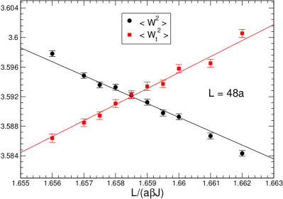
Determination of Low-Energy Parameters — In order to determine the low-energy parameters ${\cal M}_{s}$, $\rho_{s}$, and $c$ for the spin $\frac{1}{2}$ Heisenberg model on the square lattice, we have performed large-scale simulations for various inverse temperatures $\beta$ and box sizes $L$. We determine $c$ using the idea proposed in Jia10 : for a fixed box size $L$, we vary $\beta$ until the condition $\langle W_{t}^{2}\rangle=\frac{1}{2}(\langle W_{1}^{2}\rangle+\langle W_{2}^{2}\rangle)$ is satisfied. The spin wave velocity then results as $c=L/\beta$. Using this method, we obtain $c=1.6586(3)Ja$ (see figure 1).

Figure 1: The determination of $c$ using the squares of spatial and temporal winding numbers at $L=48a$.

This value is obtained by performing a weighted average over the values of $c$ listed in table I, which are extracted in volumes ranging from $L=24a$ to $L=64a$.

$L/a$	$c$
24	1.6589(6)
32	1.6586(5)
48	1.6585(5)
64	1.6585(5)

Table 1: Values of $c=L/\beta$ extracted for different lattice sizes $L/a$ by tuning $\beta$ such that the average squares of the spatial and temporal winding numbers are the same.

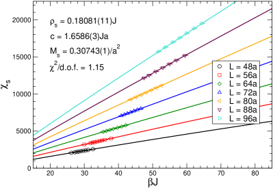
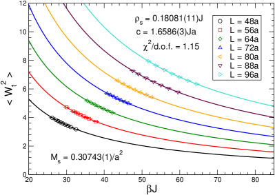
It should be noted that the above value of $c$ is consistent with the one quoted in Bea98 , but the statistical error is reduced by a factor of 7. In principle, using this method one could obtain an even more precise estimate of $c$. After obtaining this very accurate value of $c$, we carry out further large scale simulations in the cubical regime with $\beta c\approx L$. Using $c=1.6586(3)Ja$ and performing a combined fit of the Monte Carlo data for $\chi_{s}$ and $\chi_{u}$ in the cubical regime to eqs.(5) and (6), we arrive at ${\cal M}_{s}=0.30743(1)/a^{2}$ and $\rho_{s}=0.18081(11)J$ with $\chi^{2}/{\text{d.o.f.}}\approx 1$.

Figure 2: Fits of $\chi_{s}$ and $\langle W_{t}^{2}\rangle$ (and thus $\chi_{u}$) to their predicted behavior in magnon chiral perturbation theory. For better visibility, some data used in the fits are omitted in the figure.

Figure 2 illustrates the results of the fit. The main contribution to the uncertainties of ${\cal M}_{s}$ and $\rho_{s}$ results from the error of $c$ that enters the fit. Hence, with a more precise estimate of $c$, one could even further improve the accuracy of ${\cal M}_{s}$ and $\rho_{s}$. The values we obtain for $\rho_{s}$ and $c$ are more accurate than earlier estimates of these low-energy parameters. It should be noted that the value obtained for ${\cal M}_{s}$ is consistent with the one of San08 , and the statistical error is the same in both cases.

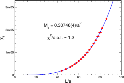
Next we simulate the model in the cylindrical regime where the condition $\beta c\gg L$ is satisfied. Since a main motivation of our study is to clarify the discrepancy between the values of ${\cal M}_{s}$ presented in Bea98 and San08 , and the accuracy we must reach is hence below the per mille level, we adopt the following strategy. First, we note that at very low temperatures $\chi_{s}$ becomes temperature-independent. In order to avoid underestimating the systematic errors in an extrapolation to zero temperature, we simulate at sufficiently low temperatures so that $\chi_{s}$ becomes independent of $\beta$ within error bars. Second, it should be noted that Monte Carlo data for $\chi_{s}$ in both the cubical Wie94 and the cylindrical regime Bea96 were used for obtaining the value of ${\cal M}_{s}$ quoted in Bea98 . Since both $\rho_{s}$ and $c$ obtained in the cubical regime are consistent with the corresponding results in the cylindrical regime, one may conclude that the overestimation of ${\cal M}_{s}=0.30797(3)/a^{2}$ presented in Bea98 is due to the cylindrical regime data for $\chi_{s}$. In order to minimize statistical correlations between $\chi_{s}$ and $\chi_{u}$, in our fitting strategy we use only cylindrical regime data for $\chi_{s}$ and cubical regime data for $\chi_{u}$. Applying these strategies and using $c=1.6586(3)Ja$, we arrive at ${\cal M}_{s}=0.30746(4)/a^{2}$ and $\rho_{s}=0.18081(11)J$ (see figure 3).

Figure 3: Fit of Monte Carlo data for $\chi_{s}$ in the cylindrical regime to their chiral perturbation theory prediction.

It should be noted that this value of ${\cal M}_{s}$, which we obtain in the cylindrical regime, is consistent with the value determined in the cubical regime. It is also consistent with the most accurate result for ${\cal M}_{s}$ that was previously obtained San08 .

In the cylindrical regime, simulating larger lattices is necessary in order to reach the same accuracy for ${\cal M}_{s}$ as the one obtained in San08 . This demonstrates the advantage of finite-temperature simulations: applying the effective field theory predictions to finite-temperature data, which can be obtained with a moderate computational effort, one achieves a very precise numerical value for ${\cal M}_{s}$. Using $c=1.6586(3)Ja$, we arrive at ${\cal M}_{s}=0.30743(1)/a^{2}$ and $\rho_{s}=0.18081(10)J$ from a combined fit including all available data points. The accuracy of these low-energy constants is not improved compared to those obtained in the cubical regime alone. This is reasonable since only a few more data points are included in the new fit.

Finally, we would like to clarify possible reasons for the overestimation of ${\cal M}_{s}=0.30797(3)/a^{2}$ obtained in Bea98 . Because of the consistency of both $\rho_{s}$ and $c$ obtained in the cubical and cylindrical regimes Wie94 ; Bea96 , one concludes that the slight overestimation of ${\cal M}_{s}$ in Bea98 is due to the cylindrical regime data for $\chi_{s}$. In particular, in order to employ eq.(7) to determine ${\cal M}_{s}$, in Bea96 a Seeley expansion has been performed in order to extrapolate the finite-temperature $\chi_{s}$ data to their corresponding zero-temperature limit. However, terminating the Seeley series is a subtle matter. Hence, the Seeley extrapolation may lead to an underestimated systematic error if the data are outside the window in which such an extrapolation is justified. Because of this, instead of repeating the analysis performed in Bea96 , we adopt another strategy. Specifically, we again simulate the model with box sizes $L/a=10,12,14,\dots,20$ at sufficiently low temperatures so that the $\chi_{s}$ data we obtain are independent of $\beta$. A combined fit of these newly obtained data for $\chi_{s}$ at very low temperature to eq.(7) and the $\chi_{u}$ data we obtained earlier in the cubical regime to eq.(6) yields ${\cal M}_{s}=0.3070(2)/a^{2}$, $\rho_{s}=0.182(2)J$ and $c=1.66(1)Ja$ with $\chi^{2}/{\text{d.o.f.}}\approx 1.3$. While the obtained value ${\cal M}_{s}=0.3070(2)/a^{2}$ is slightly below ${\cal M}_{s}=0.30743(1)/a^{2}$, the numerical values of the low-energy parameters that we just obtained are indeed consistent with those found in the cubical regime calculations Wie94 . Therefore we conclude that the overestimation of ${\cal M}_{s}$ in Bea98 is most likely due to an underestimated systematic error of $\chi_{s}$ related to the termination of the Seeley expansion used in Bea96 .

Conclusions — In this letter, we have revisited the spin $\frac{1}{2}$ Heisenberg model on the square lattice. In particular, we have refined the numerical values of the corresponding low-energy parameters, namely the staggered magnetization density ${\cal M}_{s}$, the spin stiffness $\rho_{s}$, and the spin wave velocity $c$. The spin wave velocity is determined to very high accuracy using the squares of spatial and temporal winding numbers. Remarkably, using $c=1.6586(3)Ja$ together with 2-loop magnon chiral perturbation theory predictions for $\chi_{s}$ and $\chi_{u}$ in the cubical regime, we obtained a good fit of more than 150 data points to two analytic expressions with only two unknown parameters. Specifically, from the fit we obtain ${\cal M}_{s}=0.30743(1)/a^{2}$ and $\rho_{s}=0.18081(11)J$ with $\chi^{2}/{\text{d.o.f.}}\approx 1$. The precision of ${\cal M}_{s}=0.30743(1)/a^{2}$ is comparable to the one in San08 which was obtained by an unconstrained polynomial fit using up to third or fourth powers of $1/L$. Furthermore, the data used in San08 were obtained at much larger $L$ than those used in our study. Thanks to the accurate predictions of magnon chiral perturbation theory, it requires only moderate computing resources to reach fraction of a per mille accuracy for the low-energy parameters. This is encouraging for QCD where such accuracy is mandatory to reach a sufficiently precise determination of the fundamental low-energy parameters of the strong interaction. If calculations in the chiral limit would become feasible, the experience gained in the Heisenberg model would suggest that the hyper-cubical $\varepsilon$-regime would be best suited for extracting the low-energy parameters. We have also resolved the puzzle of the per mille level discrepancy between the two values for ${\cal M}_{s}$ presented in Bea98 and San08 by re-simulating the model in the cylindrical regime. Based on a combined fit of $\chi_{s}$ in the cylindrical regime and $\chi_{u}$ in the cubical regime, we arrived at ${\cal M}_{s}=0.30746(4)/a^{2}$, which is consistent with both the results of Wie94 and San08 . The consistency of the values for ${\cal M}_{s}$ obtained in the cubical and in the cylindrical regime is particularly remarkable in view of the increased analytic 2-loop accuracy in the cylindrical regime Nie10 , which demonstrates the quantitative correctness of magnon chiral perturbation theory in describing the low-energy physics of the underlying microscopic model. Finally, we concluded that the small discrepancy in the values for ${\cal M}_{s}$ between Bea98 and San08 may be attributed to the termination of the Seeley expansion used in obtaining the former result.

We like to thank F. Niedermayer for very helpful discussions. Partial support from NSC and NCTS (North) as well as from the Schweizerischer Nationalfonds is acknowledged. The “Albert Einstein Center for Fundamental Physics” at Bern University is supported by the “Innovations- und Kooperationsprojekt C-13” of the Schweizerische Universitätskonferenz (SUK/CRUS).

References

- (1) S. Chakravarty, B. I. Halperin, and D. R. Nelson, Phys. Rev. B39 (1989) 2344.
- (2) H. Neuberger and T. Ziman, Phys. Rev. B39 (1989) 2608.
- (3) P. Hasenfratz and H. Leutwyler, Nucl. Phys. B343 (1990) 241.
- (4) P. Hasenfratz and F. Niedermayer, Phys. Lett. B268 (1991) 231.
- (5) P. Hasenfratz and F. Niedermayer, Z. Phys. B92 (1993) 91.
- (6) U.-J. Wiese and H.-P. Ying, Z. Phys. B93 (1994) 147.
- (7) B. B. Beard and U.-J. Wiese, Phys. Rev. Lett. 77 (1996) 5130.
- (8) A. W. Sandvik, Phys. Rev. B56 (1997) 18.
- (9) B. B. Beard, R. J. Birgeneau, M. Greven, and U.-J. Wiese, Phys. Rev. Lett. 80 (1998) 1742.
- (10) A. W. Sandvik, Phys. Rev. Lett. 83 (1999) 3069.
- (11) Y. J. Kim and R. Birgeneau, Phys. Rev. B62 (2000) 6378.
- (12) L. Wang, K. S. D. Beach, and A. W. Sandvik, Phys. Rev. B73 (2006) 014431.
- (13) A. W. Sandvik and H. G. Evertz, Phys. Rev. B82 (2010) 024407.
- (14) S. Wenzel, L. Bogacz, and W. Janke, Phys. Rev. Lett. 101 (2008) 127202.
- (15) F.-J. Jiang, F. Kämpfer, and M. Nyfeler, Phys. Rev. B80 (2009) 033104.
- (16) U. Gerber, C. P. Hofmann, F.-J. Jiang, M. Nyfeler, and U.-J. Wiese, JSTAT (2009) P03021.
- (17) H. G. Evertz, G. Lana, and M. Marcu, Phys. Rev. Lett. 70 (1993) 875.
- (18) F. Niedermayer and C. Weiermann, arXiv:1006.5855.
- (19) M. Göckeler and H. Leutwyler, Nucl. Phys. B350 (1991) 228.
- (20) M. Göckeler and H. Leutwyler, Phys. Lett. B253 (1991) 193.
- (21) F.-J. Jiang, arXiv:1009.6122.