Reconstructing the massive black hole cosmic history through gravitational waves

Abstract

The massive black holes we observe in galaxies today are the natural end-product of a complex evolutionary path, in which black holes seeded in proto-galaxies at high redshift grow through cosmic history via a sequence of mergers and accretion episodes. Electromagnetic observations probe a small subset of the population of massive black holes (namely, those that are active or those that are very close to us), but planned space-based gravitational-wave observatories such as the Laser Interferometer Space Antenna (LISA) can measure the parameters of “electromagnetically invisible” massive black holes out to high redshift. In this paper we introduce a Bayesian framework to analyze the information that can be gathered from a set of such measurements. Our goal is to connect a set of massive black hole binary merger observations to the underlying model of massive black hole formation. In other words, given a set of observed massive black hole coalescences, we assess what information can be extracted about the underlying massive black hole population model. For concreteness we consider ten specific models of massive black hole formation, chosen to probe four important (and largely unconstrained) aspects of the input physics used in structure formation simulations: seed formation, metallicity “feedback”, accretion efficiency and accretion geometry. For the first time we allow for the possibility of “model mixing”, by drawing the observed population from some combination of the “pure” models that have been simulated. A Bayesian analysis allows us to recover a posterior probability distribution for the “mixing parameters” that characterize the fractions of each model represented in the observed distribution. Our work shows that LISA has enormous potential to probe the underlying physics of structure formation.

I Introduction

In $\Lambda$CDM cosmologies, structure formation proceeds in a hierarchical fashion wr78 , in which massive galaxies are the result of several merging events involving smaller building blocks. In this framework, the massive black holes (MBHs) we see in today’s galaxies are expected to be the natural end-product of a complex evolutionary path, in which black holes seeded in proto-galaxies at high redshift grow through cosmic history via a sequence of MBH-MBH mergers and accretion episodes kh00 ; vhm03 . Hierarchical models for MBH evolution, associating quasar activity to gas-fueled accretion following galaxy mergers, have been successful in reproducing several properties of the observed Universe, such as the present day mass density of nuclear MBHs and the optical and X-ray luminosity functions of quasars haiman2000 ; kauffmann2000 ; wyithe2003 ; vhm03 ; croton2005 ; m07 ; dimatteo2008 .

However, only a few percent of galaxies host a quasar or an active galactic nucleus (AGN), while most galaxies harbor MBHs in their centers, as exemplified by stellar- and gas-dynamical measurements that led to the discovery of quiescent MBHs in almost all bright nearby galaxies mago98 , including the Milky Way gil09 . Our current knowledge of the MBH population is therefore limited to a small fraction of MBHs: either those that are active, or those in our neighborhood, where stellar- and gas-dynamical measurements are possible. Gravitational wave (GW) observatories can reveal the population of electromagnetically “black” MBHs.

LISA will be capable of accurately measuring the parameters of individual massive black hole binaries (MBHBs), such as their masses and luminosity distance, allowing us to track the merger history of the MBH population out to large redshifts. MBHB mergers have been one of the main targets of the LISA mission since its conception (see e.g. Hughes:2001ya ). Several authors have explored how spins, higher harmonics in the GW signal and eccentricity affect parameter estimation and in particular source localization, which is fundamental to search for electromagnetic counterparts (see, for example, the work by the LISA parameter estimation taskforce Arun:2008zn and references therein). Most work on parameter estimation has focused on inspiral waveforms, but ringdown observations can also provide precise measurements of the parameters of remnant MBHs resulting from a merger, and even test the Kerr nature of astrophysical MBHs Berti:2005ys . Initial studies using numerical relativity waveforms suggest that mergers will improve the signal-to-noise ratio of individual events and the localization accuracy of LISA McWilliams:2009bg .

While highly precise measurements for individual systems are interesting and potentially very useful for making strong-field tests of general relativity, it is the properties of the set of MBHB mergers that are observed which will carry the most information for astrophysics. To date, most of the body of work considering observations of more than one MBHB system has focused on the use of MBHBs as “standard sirens” Holz:2005df to probe the expansion history of the Universe. For a subset of the observed binaries, LISA may have sufficient angular resolution to make follow-up electromagnetic observations feasible. If the host galaxy or galaxy cluster can be identified, this will allow LISA to measure the dark energy equation of state to levels comparable to those expected from other dark energy missions Arun:2007hu . The effectiveness of LISA as a dark energy probe is limited by weak lensing VanDenBroeck:2010fp , but this can be mitigated to some extent Hilbert:2010am , and a combination of several GW detections may still provide useful constraints on the dark energy equation of state Babak:2010ej .

GW observations of multiple MBHB mergers could also be combined to extract useful astrophysical information about their formation and evolution through cosmic history. As already mentioned, our access to the MBH population in the Universe is limited to AGNs or to quiescent MBHs in nearby galaxies. In this sense we are probing only the tip of the iceberg. Theoretical astrophysicists have developed a large variety of MBH formation models vhm03 ; kbd04 ; ln06 ; bvr06 ; bv10 that are compatible with observational constraints. However, the natural lack of observations of faint objects at high redshifts and the difficulties in measuring MBH spins leave a lot of freedom in modelling MBH seed formation and mass accretion. In the last decade, several authors have employed different MBH formation and evolution models to make predictions for future GW observations, focusing in particular on LISA  wl03 ; s04 ; s05 ; svh07 ; eno04 ; rw05 . This effort has been very valuable, and established the detection of a large population of MBH binaries as one of the cornerstones of the LISA mission.

In this paper we tackle the inverse problem: we do not ask what astrophysics can do for LISA, but what LISA can do for astrophysics. In particular, we ask the following question: can we discriminate among different MBH formation and evolution scenarios on the basis of GW observations only? More ambitiously, given a set of observed MBHB coalescences, what information can be extracted about the underlying MBH population model? For example, will GW observations tell us something about the mass spectrum of the seed black holes at high redshift that are inaccessible to conventional electromagnetic observations, or about the poorly understood physics of accretion? Such information cannot be gleaned from a single GW observation, but it is encoded in the collective properties of the whole detected sample of coalescing binaries. In this paper we describe a method to extract this information in order to make meaningful astrophysical statements. The method is based on a Bayesian framework, using a parametric model for the probability distribution of observed events.

The paper is organized as follows. Section II presents the general framework of our analysis. There we review the MBH formation models considered in this paper and explain how these models translate into a theoretically observable distribution via a “transfer function” that depends (for a given source) on the detector characteristics and on the assumed model for the gravitational waveform. We describe how to sample MBH distributions via Monte Carlo methods, and how to interpret the observations in a Bayesian framework. In Section III we apply these statistical methods to the problem of deciding, given a set of LISA observations, whether we can correctly tell the true model from an alternative, for each pair in our family of MBH formation models. We focus in particular on specific comparisons that would allow us to set constraints on the main uncertainties in the input physics: namely, the seed formation mechanism, the redshift distribution of the first seeds, the efficiency of accretion during each merger and the geometry of accretion. In Section IV we describe how to go beyond a simple catalog of pure models, either by introducing phenomenological mixing parameters (designed to gauge the relative importance of different physical mechanisms in the birth and growth of MBHs) between the pure models, or by consistently implementing a mixture of different physical assumptions in a merger tree simulation. In Section V we explore how well a “consistently mixed” model can be recovered as a superposition of pure models with the phenomenological mixing parameters. In the conclusions we point out possible extensions of our work. Appendix A provides details of our treatment of errors (due to instrumental noise, uncertainties in cosmological parameters and weak lensing) in the MBHB observations. Appendix B compares parameter estimation calculations that do, or do not, take into account the orbital motion of LISA. The results suggest that angle-averaged codes that do not take into account the orbital motion may reduce computational requirements in Monte Carlo simulations, while still providing reasonable estimates of at least some binary parameters.

II Massive black holes: formation models, gravitational wave observations and their interpretation

Our goal is to assess the effectiveness of GW observations in extracting useful information about the evolution of the MBH population in the Universe. Recent work by Plowman et al. plowman09 ; plowman10 attempted to address the same question. Here we use different techniques, which improve on their analysis in several ways. Plowman et al. used the non-parametric Kolmogorov-Smirnov (KS) test to compare distributions of model parameters between models. This limited their comparisons to two parameters at a time, as higher-dimensional KS tests are not known. We instead use a parametric model by considering the number of events in any given part of parameter space to be drawn from a Poisson probability distribution. This allows us to use a Bayesian framework for the analysis. Such a framework will be important for the analysis of the actual LISA observations once these have been made, and it can be applied to a parameter space of any dimension.

In Ref. Gair:2010bx we used similar techniques to compare the same four models that were considered by Plowman et al., which were the models used for LISA parameter estimation accuracy studies in Ref. Arun:2008zn . In this paper we go considerably further by considering six additional models, chosen to probe four key aspects of the input physics used in structure formation simulations: seed formation, metallicity “feedback”, accretion efficiency and accretion geometry. In addition, we consider for the first time “model mixing”. The idea is to assume that the observed population is drawn from some combination of the “pure” models that have been simulated. The Bayesian framework allows us to recover a posterior probability distribution for the “mixing parameters” that characterize the fraction of each model represented in the observed distribution. Such an analysis is not possible in the KS framework. The model mixing analysis is very important, as the real Universe is most certainly not drawn from any of the idealized models that currently exist. The mixing parameters will reflect the relative contributions in the true Universe of the different input physics in the pure models.

For our analysis, we adopt the following strategy:

• We consider a set of MBH formation and evolution models predicting different coalescing MBHB theoretical distributions (Section II.1);

• To account for detection incompleteness, we filter the distribution predicted by each model using a detector “transfer function” that produces the observed theoretical distributions under some specific assumptions about the GW detector (Section II.2). This is basically the distribution one would observe assuming an infinite number of detections;

• We generate Monte Carlo realizations of the coalescing MBHB population from one of the models (Section II.3) or from a mixture of models (Section IV), and simulate GW observations of the inspiralling binaries, including errors in the source parameter estimation;

• We then compare (in a statistical sense) the catalog of observed events – including measurement errors – with the observed theoretical distributions, to assess at what level of confidence we can recover the parent model. The statistical methods we use are detailed in Section II.4.

In this paper we will consider the Laser Interferometer Space Antenna (LISA) as an illustrative case, but the strategy outlined above can easily be generalized to other proposed space-borne GW observatories, such as ALIA, DECIGO or BBO BBO ; Crowder:2005nr ; Ando:2010zz .

An important caveat is that, for a source at redshift $z$, GW observations do not measure the binary parameters in the source frame, but rather the corresponding redshifted quantities in the detector frame. For this reason, throughout the paper we shall characterize MBHBs via their redshifted parameters. Given a MBHB with rest-frame masses $M_{1,r}>M_{2,r}$, the masses in the detector frame are given by $M_{1}=(1+z)M_{1,r}$, $M_{2}=(1+z)M_{2,r}$. In terms of these masses we can also define (as is the custom in GW physics) the total mass $M=M_{1}+M_{2}$, the mass ratio $q=M_{2}/M_{1}$, the symmetric mass ratio $\eta=M_{1}M_{2}/M^{2}$ and the chirp mass ${\cal M}=\eta^{3/5}M$. In our calculations we assume a concordance $\Lambda$CDM cosmology characterized by $H_{0}=70$km s^-1 Mpc^-1, $\Omega_{M}=0.27$ and $\Omega_{\Lambda}=0.73$.

For simplicity we will focus on the inspiral of circular, non-spinning binaries; therefore, each coalescing MBHB in our populations will be characterized by only three intrinsic parameters ($z$, $M$ and $q$). In terms of gravitational waveform modelling, the results presented here can be considered conservative. Different accretion models may result in different MBH spin distributions. Including spin in the analysis will provide additional information that will help to further constrain the physical mechanisms at work in shaping the MBH population model Berti:2008af ; plowman10 . The inclusion of the merger/ringdown portion of the signal will increase the signal-to-noise ratio (SNR) of observed binaries and allow measurements of the parameters of the merger remnants, providing additional information on the mechanisms responsible for MBH growth.

In the following subsections we will introduce all the elements and methodologies relevant to our analysis.

II.1 Cosmological massive black hole populations

The assembly of MBHs is reconstructed through dedicated Monte Carlo merger tree simulations vhm03 which are framed in the hierarchical structure formation paradigm. Each model is constructed by tracing the merger hierarchy of $\sim$200 dark matter halos in the mass range $10^{11}-10^{15}M_{\odot}$ backwards to $z=20$, using an extended Press & Schechter (EPS) algorithm (see vhm03 for details). The halos are then seeded with black holes and their evolution is tracked forward to the present time. Following a major merger (defined as a merger between two halos with mass ratio $M_{h_{2}}/M_{h_{1}}>0.1$, where $M_{h_{2}}$ is the mass of the lighter halo), MBHs accrete efficiently an amount of mass that scales with the fifth power of the host halo circular velocity and that is normalized to reproduce the observed local correlation between MBH mass and the bulge stellar velocity dispersion (the $M-\sigma$ relation, see tr02 and references therein). For each of the simulated halos, all of the binary coalescences that occur are stored in a catalog. The results for each halo are then weighted using the EPS halo mass function and are numerically integrated over the observable volume shell at every redshift to obtain the coalescence rate of MBHBs as a function of black hole masses and redshift (see, e.g., Fig. 1 in svh07 ). We then find the theoretical distribution of (potentially) observable coalescing binaries by multiplying the rate by the LISA mission lifetime (here assumed to be three years) to obtain the distribution ${\cal N}_{i}\equiv d^{3}N_{i}/dzdMdq$, where the index $i$ labels the MBH formation model.

In the general picture of MBH cosmic evolution, the MBH population is shaped by the details of the seeding process and the accretion history. Both issues are poorly understood, and largely unconstrained by present observations. We identify four key factors that have a direct impact on specific observable properties of the merging MBHB population:

1. the seed formation mechanism shapes the initial seed mass function;

2. the impact of metallicity on MBH formation determines the redshift distribution of the seeds;

3. the accretion efficiency determines the growth rate of MBHs over cosmic history;

4. the accretion geometry is crucial in the evolution of the MBH spins.

We explore different formation scenarios by considering two different prescriptions for each of the elements in the above list, as follows:

Name	$i$	Seeding	Metallicity	Accretion model	Accretion geometry	$\bar{N}_{i}$ $[yr^{-1}]$
VHM-noZ-Edd-co	1	POPIII	$Z=0$	Eddington	coherent	86
VHM-noZ-Edd-ch	2	POPIII	$Z=0$	Eddington	chaotic	81
VHM-Z-Edd-co	3	POPIII	all Z	Eddington	coherent	108
VHM-Z-Edd-ch	4	POPIII	all Z	Eddington	chaotic	113
BVR-noZ-Edd-co	5	Quasistar	$Z=0$	Eddington	coherent	26
BVR-noZ-Edd-ch	6	Quasistar	$Z=0$	Eddington	chaotic	24
BVR-Z-Edd-co	7	Quasistar	all Z	Eddington	coherent	22
BVR-Z-Edd-ch	8	Quasistar	all Z	Eddington	chaotic	29
BVR-noZ-MH-co	9	Quasistar	$Z=0$	Merloni & Heinz	coherent	33
BVR-noZ-MH-ch	10	Quasistar	$Z=0$	Merloni & Heinz	chaotic	33

Table 1: The ten “pure” MBH population models considered in this paper. For convenience, in the following we will identify models by the integer, $i$, listed in the second column. In the last column, $\bar{N}_{i}$ denotes the predicted coalescence rate.

1. The seed formation mechanism. Two distinct families of models have become popular in the last decade, usually referred to as “light” and “heavy” seed models. Here we consider two different scenarios representative of the two possibilities. (i) The “VHM” model; developed by Volonteri, Haardt & Madau vhm03 , this model is characterized by light seeds ($M\sim 100M_{\odot}$), which are thought to be the remnants of Population III (POPIII) stars, the first generation of stars in the Universe mr01 . (ii) The “BVR” model; proposed by Begelman, Volonteri & Rees bvr06 , this model belongs to the family of “heavy seed” models. Bar within bar instabilities sfb89 occurring in massive protogalactic disks trigger gas inflow toward the center, where a “quasistar” forms. The core of the quasistar collapses into a seed black hole that efficiently accretes from the quasistar envelope, resulting in a final seed black hole with mass $M\sim$ few $\times 10^{4}M_{\odot}$.

2. Metallicity “feedback”. Both of the black hole formation models described above require that a large amount of gas is efficiently transported to the halo center. The gas inflow has to occur on a timescale that is shorter than that of star formation, to avoid competition in gas consumption and disruption of the inflow process by supernovae explosions. It has been suggested that metal-free conditions are conducive to efficient gas inflow, as fragmentation is inhibited bl03 . If fragmentation is suppressed, and cooling proceeds gradually, the gaseous component can cool and contract before many stars form. The gas metallicity $Z$ is therefore an important environmental factor to take into account, and we consider two cases. (i) “noZ” models; black hole seeding is assumed to be efficient at zero metallicity only, with a sharp threshold in cosmic time. In these models, seeds form at very high redshift ($20>z>15$). (ii) “Z” models; efficient seed formation occurs also at later times. Here we treat POPIII star and quasistar black hole formation differently. We still assume that POPIII stars can form only out of metal-free gas, but we track the probability that a halo at late times is still metal-free by adopting the metal enrichment models developed in s03 . For the case of quasistars, instead, we drop the assumption of zero metallicity. This choice is motivated by recent high-resolution numerical simulations of gas-rich galaxies at solar metallicities (e.g. mayer10 ), which show that bar within bar instabilities can drive a significant amount of gas to the central nucleus before star formation quenches the inflow. These models are characterized by seed formation also at later times, in metal enriched halos. See bv10 for full details on the model and its implementation.

3. The accretion efficiency. MBHs powering AGNs exhibit a broad phenomenology; they accrete at different rates, with different efficiencies and luminosities (see mh08 and references therein). In the absence of a solid coherent theory for describing the accretion process, several toy models are viable, and we consider two of these models. (i) “Edd” accretion model; the easiest possible recipe is to assume that accretion occurs at the Eddington rate, parametrized through the Eddington ratio $f_{e}$ (we take $f_{e}=0.3$ in our models). (ii) “MH” accretion model; we also use a more sophisticated scheme combining low and high accretion rates, as described by Merloni & Heinz mh08 .

4. The geometry of accretion. Standard accretion disks are unstable to self gravity beyond a few thousands of Schwarzschild radii tom64 . It is therefore not guaranteed that the supply of gas to the central black hole will be continuous, smooth and planar. We consider two different scenarios. (i) Coherent accretion (“co” models); the flow of material that feeds the black hole is assumed to be continuous, smooth and planar. Accretion is a single steady episode lasting about a Salpeter time. (ii) Chaotic accretion (“ch” models); in this scenario, proposed by King & Pringle kp06 , a single accretion event is made of a collection of short-lived accretion episodes, and the angular momentum of each accreted matter clump is randomly oriented. These accretion models primarily lead to different expectations for the black hole spins: intermediate-high, $a\sim 0.6-0.9$, in the coherent case; low, $a<0.2$, in the chaotic case Berti:2008af . In this work we ignore black hole spin in the modelling of gravitational waveforms, and therefore we do not assess the impact of spin measurements in resolving different MBH formation scenarios. However, the accretion prescription also leaves an imprint on the component masses. The models assume that the mass-to-energy conversion efficiency, $\epsilon$, depends on black hole spin only, so the two models predict different average efficiencies of $\sim 20\%$ and $\sim 10\%$, respectively. The mass-to-energy conversion directly affects mass growth, with high efficiency implying slow growth, since for a black hole accreting at the Eddington rate the black hole mass increases with time as

   $$M(t)=M(0)\,\exp\left(\frac{1-\epsilon}{\epsilon}\frac{t}{t_{\rm Edd}}\right)\,,$$ (1)

   where $t_{\rm Edd}=0.45$Gyr. The “coherent” versus “chaotic” models thus allow us to study how different growth rates affect LISA observations.

By choosing two different prescriptions for each of the four pieces of input physics listed above we built ten different MBH population models, which are summarized in Table 1. We shall refer to these models as “pure”, in the sense that we do not mix different recipes for seed formation and accretion history (e.g., accretion is either coherent or chaotic, etc.). We will consider “mixed” models in Section IV. It is worth emphasizing that all of these models successfully reproduce various properties of the observed Universe, such as the present-day mass density of nuclear MBHs and the optical and X-ray luminosity functions of quasars. GW observations may therefore provide an invaluable tool to constrain the birth and growth of MBHs, particularly at high redshift.

Figure 1: Transfer function for the case $\rho_{\rm thr}=8$ and observation with two interferometers, for $z=0.5,\,2,\,5,\,10,\,15,\,20$.

II.2 Theoretically observable distributions: the transfer function

In order to compare a set of observed events to a given MBH population model, we must map the coalescence distribution predicted by the model to a theoretically observable distribution which takes into account the “incompleteness” of the observations resulting from the limited sensitivity of any given GW detector. This information can be encoded in a transfer function $T(z,M,q)$, that depends only on the detector characteristics and on the gravitational waveform model.

We model the detector and the gravitational waveform following Refs. Berti:2004bd ; Berti:2005qd . The detector response is modelled following Cutler Cutler:1997ta : the three-arm LISA constellation is thought of as a superposition of a pair of linearly independent two-arm right-angle interferometers, and we can estimate the effect of “descoping options” or a failure on one satellite by assuming that only one of the two detectors is operational. The MBHB inspiral signal is modelled using the restricted post-Newtonian approximation, truncating the GW phasing at second post-Newtonian order – i.e., at order $(v/c)^{4}$, where $v$ is the binary orbital velocity. We also limit our analysis to circular inspirals of nonspinning MBHs and neglect contributions to the observable signal that come from higher harmonics in the inspiral signal and from the (gravitationally loud) merger/ringdown phase. The latter assumption significantly underestimates the energy carried in the GWs Berti:2007fi , the SNR of the signal McWilliams:2010eq and the accuracy in estimating the source parameters McWilliams:2009bg . From the point of view of studying MBH populations, it also means that we discard all information on the mass and spin distribution of MBHs formed as a result of each merger Berti:2005ys . In this sense, our assessment of the potential of LISA to constrain MBH formation models should be considered conservative.

An important advantage of working in the frequency domain and of adopting a simplified waveform model is that we can sample the three-dimensional space $(z,M,q)$ by fast Monte Carlo simulations using an adaptation of the Fortran code described in Berti:2004bd . Typically, we can estimate SNRs and parameter estimation errors of $\sim 10^{6}$ binaries in one day on a single processor. This would not be possible with a more complex time-domain code including spin dynamics, such as that used in plowman10 . We consider a $21\times 21\times 21$ three-dimensional grid spaced logarithmically in the intervals $q\in[10^{-3},1]$, $M\in[10^{3},10^{8}]$, and approximately linearly in $z$ (namely, we consider $z=0.5$ and then all values of $z=1,\dots,20$ in steps of $\Delta z=1$), for a total of 9261 points. At each point, we generate 1000 binaries assuming random position in the sky and orientation, random phase at coalescence, and coalescence time $t_{c}$ in the range [0, 3yr] (i.e., we consider only events that coalesce during the LISA mission). The GW signal is calculated in the Fourier domain in the stationary phase approximation. Our statistical analysis, which will be discussed in section II.4, includes parameter measurement errors, which are modelled as described in Appendix A. The modelling of errors due to instrumental noise relies on the computation of the so-called Fisher information matrix Vallisneri:2007ev . For each system we compute the Fisher matrix and its inverse by means of the LU decomposition, as described in Berti:2004bd . The accuracy of the inversion is usually worse for certain values of the intrinsic parameters and of the angular position/orientation of the binary. We discard “bad” Fisher matrix inversions by monitoring a quantity $\epsilon_{\rm inv}$, defined as

$$\epsilon_{\rm inv}=\max_{i,j}|I^{\rm num}_{ij}-\delta_{ij}|\,,$$ (2)

where $I^{\rm num}_{ij}$ is the “numerical” identity matrix obtained by multiplying the inverse matrix by the original, and $\delta_{ij}$ is the standard Kronecker delta symbol Berti:2004bd . We set a maximum tolerance of $\epsilon_{\rm inv}=10^{-3}$ to accept the inversion. For the accepted events, we compute the SNR $\rho$ and then we define the transfer function as

$$T(z,M,q)=\frac{N(\rho>\rho_{\rm thr})}{N}\,,$$ (3)

where $N=1000$ is the number of successful matrix inversions at any given grid point and $N(\rho>\rho_{\rm thr})$ is the number of binaries fulfilling the condition $\rho>\rho_{\rm thr}$, where $\rho_{\rm thr}$ is a pre-specified SNR threshold.

We consider four transfer functions $T_{j}(z,M,q)$ ($j=1,2,3,4$) according to the following prescriptions: (1) one interferometer, $\rho_{\rm thr}=8$; (2) one interferometer, $\rho_{\rm thr}=20$; (3) two interferometers, $\rho_{\rm thr}=8$; (4) two interferometers, $\rho_{\rm thr}=20$. The chosen thresholds correspond (roughly) to the minimum SNR for which we expect to be able to claim a confident detection ($\rho_{\rm thr}=8$) and the minimum SNR for which we expect to obtain a decent accuracy in estimating the parameters of the source ($\rho_{\rm thr}=20$). Note that, by definition, $0\leq T(z,M,q)\leq 1$.

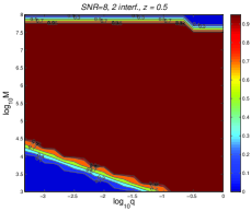
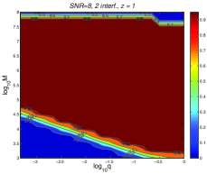
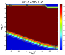
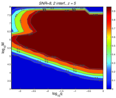
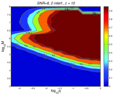
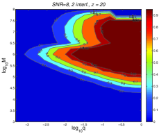
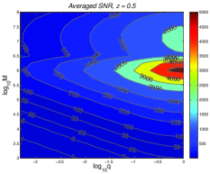
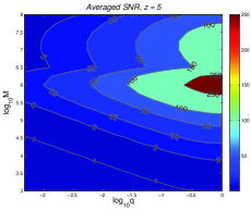
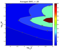
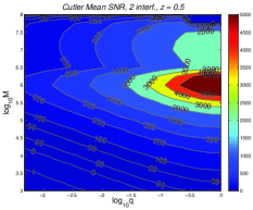
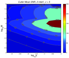
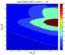
Examples of $T_{3}(z,M,q)$ in the $(M,q)$ plane at different redshifts are shown in Figure 1. As expected, the transfer function is close to unity in the whole of the $(M,q)$ plane at low redshifts, but a smaller number of events are observable as we consider binaries coalescing at higher redshifts. When we remember that high redshifted masses correspond to low observation frequencies, it is easy to understand that the characteristic shape of the contour plots for large redshift (say, $z=20$) reflects the shape of the LISA sensitivity curve (cf. Figure 1 of Ref. Berti:2004bd ). More details of the calculation of SNRs and parameter estimation errors in the three dimensional space $(M\,,q\,,z)$ are given in Appendix B.

The transfer functions are coupled to the event distributions predicted by the models to obtain the theoretically observable distributions $N_{T}(z,M,q)$ for each model under the different assumptions on the transfer function; namely,

$$N_{T_{i,j}}(z,M,q)=\frac{d^{3}N_{i}}{dzdMdq}\times T_{j}(z,M,q)\,,$$ (4)

where $i$ labels the MBH population model being considered and $j$ labels the assumed detector specifics. These are the distributions which should be compared to simulated observed catalogs of MBHBs.

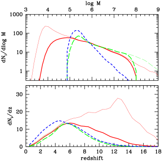
For illustration, in Figure 2 we compare the marginalized distributions

$$\frac{dN_{i}}{dM}=\int dz\int dq\,\frac{d^{3}N_{i}}{dzdMdq}\quad{\rm and}$$

$$\frac{dN_{i}}{dz}=\int dM\int dq\,\frac{d^{3}N_{i}}{dzdMdq}$$ (5)

(thin lines) with the corresponding marginalized distributions

$$N_{T_{i,3}}(M)=\int dz\int dq\,N_{T_{i,3}}(z,M,q)\quad{\rm and}$$

$$N_{T_{i,3}}(z)=\int dM\int dq\,N_{T_{i,3}}(z,M,q)$$ (6)

(thick lines). Note that for some of the heavy seed models (namely, the short-dashed line corresponding to model BVR-noZ-MH-co) the two curves perfectly overlap: in these cases LISA observations do not miss events, i.e. they are “complete”.

Figure 2: Examples of the marginalized distributions $dN_{i}/dM$ (upper panel) and $dN_{i}/dz$ (lower panel) predicted by different MBH formation models. In each panel we plot the following models: VHM-noZ-Edd-co (solid red lines); BVR-noZ-Edd-ch (long-dashed green lines); BVR-noZ-MH-co (short-dashed blue lines). Thin lines represent the coalescence distributions predicted in three years, while thick lines represent the theoretically observable distributions after the transfer function $T_{3}(z,M,q)$ has been applied, namely $N_{T_{i,3}}(M)$ and $N_{T_{i,3}}(z)$ (see text for details).

II.3 Synthetic Monte Carlo catalogs

To simulate LISA observations we perform 1000 Monte Carlo samplings of the $d^{3}N_{i}/dzdMdq$ distribution predicted by each model, producing 1000 catalogs of coalescing binaries over a period of three years. In each catalog, the source position in the sky and the direction of the orbital angular momentum are assumed to be uniformly distributed. The phase at coalescence $\Phi_{c}$ and the coalescence time $t_{c}$ are randomly chosen in the range [0, $2\pi$] and [0, 3yrs], respectively. Each waveform is described by the set of parameters

$$\Theta=(\log A,\log{\cal M},\log\eta,t_{c},\Phi_{c},\theta_{S},\Phi_{S},\theta_{L},\Phi_{L}),$$ (7)

where $(t_{c},\Phi_{c})$ are the phase and time of coalescence, $(\theta_{S},\Phi_{S})$ represents the source location in ecliptic coordinates, $(\theta_{L},\Phi_{L})$ give the orientation of the orbital angular momentum of the binary and the GW amplitude of the signal

$$A\propto\frac{{\cal M}_{z}^{5/6}}{D_{L}}\,,$$ (8)

where

$$D_{L}=\frac{1+z}{H_{0}}\int_{0}^{z}\frac{dz^{\prime}}{(1+z^{\prime})^{2}[\Omega_{M}(1+z^{\prime})^{3}+\Omega_{\Lambda}]^{1/2}}$$ (9)

is the luminosity distance to the source. Our theoretical distributions are not functions of $(M,\eta,D_{L})$, but rather functions of ($M,q,z$), and the mapping between the two sets of parameters is given in Appendix A.

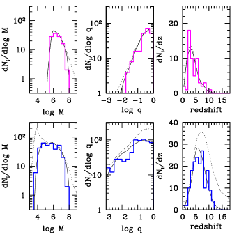
LISA measurements will yield a set of data $\{D_{k}\}$, $k=1,\dots,N$, where $N$ is drawn from a Poisson distribution with mean $\bar{N}_{i}$ coincident with the theoretical number of events predicted by the model we consider (cf. Table 1). Each element in the set is described by $(\bar{z},\sigma_{z};\bar{M},\sigma_{M};\bar{q},\sigma_{q})$, where $\bar{z}$, $\bar{M}$, $\bar{q}$ are the true parameters of the system and $\sigma_{z}$, $\sigma_{M}$, $\sigma_{q}$ are the diagonal elements of the variance-covariance matrix describing the measurement errors. The latter are computed as described in Appendix A and include contributions from instrumental noise, from uncertainties in cosmological parameters and from weak lensing. We approximate the covariance matrix as diagonal since this is conservative, and the covariances are generally small. Strictly speaking we are not justified in ignoring the large covariance between any two mass parameters (say, $M$ and $\eta$); however the errors on the mass parameters are always negligible when compared with errors on luminosity distance, cosmological parameters and weak lensing (see Appendix A). The probability density function for the measured source parameters is then a multivariate Gaussian with these standard deviations, centred at the true source parameters. As discussed in the next section, the errors can be folded into the analysis in two ways. The one we adopt is to construct the theoretically observable distribution, ${\cal N}_{i,j}(z,M,q)$ as described in Section II.2, by spreading each source over multiple bins according to the Gaussian probability distribution for the measurement errors. We then construct data sets by assigning a unique set of observed parameters to each event that is equal to the true parameters, plus a random error drawn from the same probability distribution. For each “pure” MBH population model (label “$i$”) and LISA transfer function (label “$j$”), we produce 1000 of these “observed” datasets $\{D_{k}\}_{i,j}$, to compare to the theoretically observable distributions. Examples of Monte Carlo generated datasets are shown in Figure 3.

Figure 3: Examples of Monte Carlo generated datasets. The left panels show the $dN_{i}/dM$ distributions, the central panels show the $dN_{i}/dq$ distributions and the right panels show the $dN_{i}/dz$ distributions. The upper panels refer to model BVR-Z-Edd-co, the lower panels to model VHM-Z-Edd-co. In each panel the dotted curves represent the theoretical distributions, and the solid curves represent the theoretically observable distribution filtered with the transfer function $T_{3}$. The thick histograms show one Monte Carlo realization of the theoretical distribution, as observed by LISA, under the assumption of two operational interferometers and $\rho_{\rm thr}=8$.

Throughout our study, we will assume $T_{\rm obs}=3$ yrs as the fiducial LISA mission lifetime. However, it is interesting to study how the performance of LISA improves as a function of the duration of the data stream used in the analysis. This problem could be particularly relevant if, as expected, there are gaps in the LISA data stream. For this reason we will consider increasing observation times, $T_{\rm obs}$, of 3 months, 6 months, 1 year, 18 months, 2 years and 3 years, respectively. To construct these reduced datasets, we just pick events from the catalog that coalesce at $t_{c}<T_{\rm obs}$, and then renormalize the theoretical distributions by a factor $T_{\rm obs}/3$yr. In doing this, we ignore sources that coalesce outside the reduced observation time, but which may have enough SNR to be detected in the shorter data segment. This is conservative since we are effectively choosing only to include the coalescing sources in our analysis. However, for MBHBs, unlike the EMRI case (see Ref. emrimodsel ), almost all of the source SNR (and, consequently, the accuracy in the determination of $M$, $q$, and $z$) is accumulated in the last month of inspiral, and so there would not be a great deal to gain by including these sources in the analysis.

II.4 Statistical analysis tools

In this work we will adopt a Bayesian approach to model selection and parameter estimation. This requires a parametric model for the distribution of events that LISA will observe. A particular astrophysical model of MBH formation cannot predict the actual number of events that will occur during the LISA mission, as the mergers will occur stochastically, but instead predicts the rate at which events with particular parameters occur. Assuming random start times, the number of events, $n_{i},$ that will be seen in a particular bin, ${\cal B}_{i}$, in parameter space will be drawn from a Poisson probability distribution with parameter $r_{i}$ equal to the rate integrated over the bin:

$$p(n_{i})=\frac{(r_{i})^{n_{i}}{\rm e}^{-r_{i}}}{n_{i}!}\,.$$ (10)

If we divide the parameter space up into a certain number of bins, $K$ say, then the information that comes from LISA (the data $D$) is the number of events in each bin. The overall likelihood, $p(D|\vec{\lambda},M)$ of seeing this data under the model $M$ with parameters $\vec{\lambda}$ is the product of the Poisson probabilities for each bin

$$p(D|\vec{\lambda},M)=\prod_{i=1}^{K}\frac{(r_{i}(\vec{\lambda}))^{n_{i}}{\rm e}^{-r_{i}(\vec{\lambda})}}{n_{i}!}\,.$$ (11)

The rates that enter this expression are the rates for observed events, i.e., the product of the intrinsic rate predicted by the model with the LISA transfer function, as discussed in the previous section. It is straightforward to take the limit of this expression as the bin sizes tend to zero to derive a continuum version of this equation emrimodsel .

LISA will not be able to measure the parameters of each system perfectly due to instrumental noise. In addition, weak lensing will introduce errors in the measurements of luminosity distance. Since we wish to use redshift rather than distance as a parameter, further errors will be introduced from imperfect knowledge of the luminosity distance-redshift relation. The modelling of these errors was mentioned earlier, and is described in detail in Appendix A. There are two ways in which the errors can be folded into the statistical analysis. Once LISA observations have been made, we will obtain posterior probability distributions for the source parameters which account for the error-induced uncertainties. The likelihood will then be computed by integrating the continuum version of Eq. (11) over the posterior, as described in emrimodsel . The second approach, which we adopt here as it is more appropriate for a priori studies of this type, is to fold the expected errors into the computation of the observed rates, $r_{i}$. In practice, we compute these rates directly from the Monte Carlo realizations described in the preceding section. For each source in the catalog we can assign fractional rates to every bin in parameter space, computed by integrating the error probability distribution for the source over that particular bin. In other words, we spread each source out into multiple bins, as predicted by the error model described earlier. When generating realizations of the LISA data set, we assign each source to one bin only, according to some “observed parameters” (which could represent, for instance, the maximum a posteriori parameters of the source). We take these observed parameters to be equal to the true parameters plus an error drawn from the same error distribution.

Given the likelihood described above, Bayes theorem allows us to assign a posterior probability, $p(\vec{\lambda}|D,M)$, to the parameters, $\vec{\lambda}$, of a model, $M$, given the observed data, $D$, and a prior, $\pi(\vec{\lambda})$, for the parameters $\vec{\lambda}$:

$$p(\vec{\lambda}|D,M)=\frac{p(D|\vec{\lambda},M)\,\pi(\vec{\lambda})}{{\cal Z}},$$

$${\cal Z}=\int p(D|\vec{\lambda},M)\,\pi(\vec{\lambda}){\rm d}^{N}\lambda.$$ (12)

When comparing two models, A and B, that could each describe the data, we can compute the odds ratio (see, for example, mackayinf )

$$O_{AB}=\frac{{\cal Z}_{A}\,P(A)}{{\cal Z}_{B}\,P(B)}\,,$$ (13)

in which $P(X)$ denotes the prior probability assigned to model $X$. If $O_{AB}\gg 1$ ($O_{AB}\ll 1$), model $A$ (model B) provides a much better description of the data.

In this paper, we will consider two types of model comparison. In Section IV, we will consider mixed models in which the observed distribution is drawn from a superposition of two or more of the underlying “pure” models. In those cases, the models depend on one or more free “mixing” parameters for which we will obtain posterior distributions using Eq. (12). First, however, in Section III, we will make direct comparisons between the pure models. In that case, the models do not have any free parameters. The odds ratio, (13), then reduces to the product of the likelihood ratio with the prior ratio

$$O_{AB}=\frac{p(D|A)}{p(D|B)}\frac{P(A)}{P(B)}.$$ (14)

The models we consider have all been tuned to match existing constraints, and so at present we have no good reason to prefer one model over the others. We therefore assign equal prior probability to each pure model, $P(A)=P(B)=0.5$, and the odds ratio becomes the likelihood ratio. We assign probability $p_{A}=p(D|A)/(p(D|A)+p(D|B))$ to model A, and $p_{B}=1-p_{A}$ to model B.

Figure 4: Two alternative ways to represent our ability to distinguish models. The left panel shows an ROC curve, while the right panel shows the CDF of the confidence achieved over multiple realizations of the correct (upper curve) and wrong (lower curve) model. More details are given in the text. The model comparison used for this figure was VHM-noZ-Edd-co to VHM-noZ-Edd-ch, for a three month LISA observation and the most pessimistic assumption ($T_{2}$) on the transfer function.

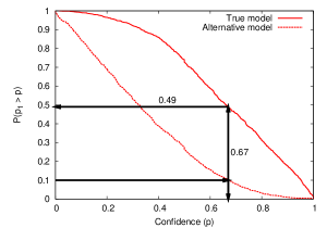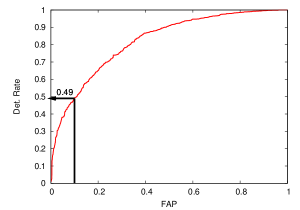
Once LISA data is available, each model comparison will yield this single number, $p_{A}$, which is our confidence that model A is correct. Since the LISA data is not currently available, we want to work out how likely it is that we will achieve a certain confidence with LISA. So, we generate 1000 realizations of the LISA data stream and look at the distribution of the likelihood ratio and confidence over these realizations. We can represent the results of this analysis in two alternative ways. These are illustrated in Figure 4, and we will refer to the two panels of this figure extensively in the following. The left panel shows a receiver operator characteristic (ROC) curve. This is a “frequentist” way to represent the data. To generate this plot, we assume that we have specified a threshold on the statistic, in this case the likelihood ratio, before the data is collected. If the value of the statistic computed for the observed data exceeds the threshold then model A is chosen, otherwise model B is chosen. For a given threshold, the frequency with which the threshold is exceeded for realizations of model B defines the false alarm probability (FAP), while the frequency with which the threshold is exceeded for realizations of model A defines the detection rate. The ROC curve shows detection rate vertically versus FAP horizontally. In the figure, we indicate how, for an FAP of $10\%$, we can find the detection rate, which in this case is $49\%$. This is the format we used to present our previous results in Ref. Gair:2010bx . While the ROC is a convenient way to represent the data, it is incomplete, in that it does not tell us by how much we exceed the threshold: the result is far more convincing if we obtain a likelihood ratio 10 times the threshold, than 1.1 times the threshold.

The right panel of Figure 4 shows an alternative representation of the same data which contains this additional information. It shows the cumulative distribution function (CDF) for the “confidence” we would have in model A, based on our observation, i.e., the probability, $p_{A}$, we assign to model A in a Bayesian interpretation of the results of an observation. The upper curve is the CDF computed over multiple realizations of model A (i.e., the horizontal axis then shows our confidence in the true model), while the lower curve shows the CDF computed from realizations of model B (i.e., the horizontal axis then shows our confidence in the wrong model). The best way to interpret this plot is to choose a certain confidence level, e.g., $p=0.95$ (approximately 2$\sigma$). The value on the upper curve is the frequency with which this confidence level, or better, would be achieved in a LISA observation when that model was correct, while the value on the lower curve at $1-p$ is the frequency with which we would not be able to rule out model A with that confidence, when it was not true.

The CDF plot encodes the same information as the ROC curve. If we assign a certain FAP, say $10\%$ as before, we draw a horizontal line at that value and find where it intersects the lower curve. This tells us the confidence level corresponding to that FAP, in this case $0.67$. The value on the upper curve at this confidence level is the detection rate at that FAP, and we find that it is $49\%$, as expected. In the current paper, we will use this second, Bayesian, representation of the results for all the remaining plots, as it encodes all of the information that can be gleaned from the Monte Carlo simulations. The Bayesian approach assigns relative probabilities to the models, rather than making a binary statement that model A is “right” or model B is “right”.

Figure 5: Comparison of performance of model selection when including the total number of events as a parameter of the model (labeled “no marginalization”) and when this parameter is marginalized over (labeled “with marginalization”). The small difference indicates that the total number of events contains relatively little information compared to the shape of the parameter distributions. We show the same model comparison as in Figure 4.

Figure 6: Results for comparisons of the pure models. Each plot shows all possible comparisons varying only one of the elements listed in Table 1. Top left panel: we consider the effect of the accretion geometry, comparing coherent to chaotic for each of the combinations of the other ingredients. Top right panel: we consider the effect of the accretion model, comparing Eddington accretion to Merloni-Heinz accretion for the BVR-noZ models. Bottom left: we consider the effect of metallicity by comparing the noZ to Z models for VHM-co, VHM-ch, BVR-co and BVR-ch. Bottom right: we consider the effect of the seeding assumption, comparing the VHM to BVR models for the four combinations noZ-co, noZ-ch, Z-co and Z-ch, each with Eddington accretion. In all panels we are making the most pessimistic assumptions about the detector, i.e., we use the transfer function $T_{2}$ (one interferometer, $\rho_{\rm thr}=20$). These results are for a 3 month LISA observation, except for the top left panel which is for a one year observation.

The models we consider differ not only in the distribution of events that they predict, but also in the total number of events. As the latter could be considered a less robust prediction of the models, we can ask whether it carries much weight for model selection. This can be done by introducing a free parameter into each model, which is an overall normalizing factor, and then marginalizing over it, i.e., integrating the posterior probability over this parameter. We write $r_{i}=N\tilde{r}_{i}$, where $\tilde{r}_{i}$ is the rate in bin $i$ for a model that predicts $1$ event in total. The probability marginalized over $N$ is

$$\tilde{p}(D|M)=\left(\prod_{i=1}^{K}\frac{\tilde{r}_{i}^{n_{i}}}{n_{i}!}\right)\sum_{n=1}^{\infty}n^{N_{\rm obs}}{\rm e}^{-n}\,,$$ (15)

where $N_{\rm obs}=\sum n_{i}$ is the total number of events observed. The summation in the second term is dependent only on $N_{\rm obs}$ and, as such, is model-independent. It can thus be seen that

$$\tilde{p}(D|M)\propto p(D|M){\rm e}^{N_{\rm M}}N_{\rm M}^{-N_{\rm obs}}\,,$$ (16)

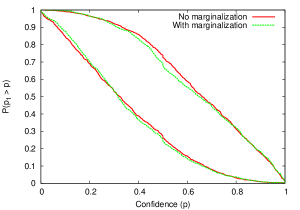
where $N_{\rm M}$ is the number of events predicted by the un-normalized model $M$. We can decouple the contribution from the total number of events and the distribution of event parameters by replacing the likelihood $p(D|M)$ by the marginalized likelihood $\tilde{p}(D|M)$ in the likelihood ratio. In Figure 5 we show the effect this has on the CDFs for the Bayesian confidence, for the comparison between model VHM-noZ-Edd-co and VHM-noZ-Edd-ch. We see that including marginalization makes very little difference to the results. This implies that the number of events predicted by a model contains little information relative to the parameter distribution. For the remaining plots in this paper, we do not marginalize over $N_{\rm M}$, but we have checked that in all cases the effect of the marginalization is small.

III Results for the pure models

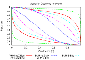
We now describe the results of our analysis. In this section we will compare pairs of pure models using the technique described in the previous section. We generated 1000 realizations for each model, as described in Section II.3. For each pair of models $A$ and $B$, we computed the CDF of the Bayesian confidence of model $A$ versus model $B$ over the realizations of model $A$ and those of model $B$. We present selected results in Figure 6 using the CDF curves described in the previous section.

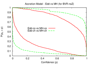
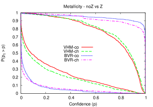
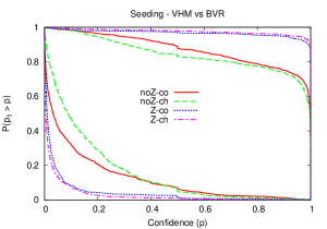
Each panel in Figure 6 shows the results for pairs of models that differed in only one of the four aspects of the input physics detailed in section II.1 and listed in Table 1. To be conservative, we consider a pessimistic scenario for the detector (transfer function $T_{2}$: one interferometer, $\rho_{\rm thr}=20$).

In the upper-left panel we show all possible (five) comparisons among pairs of models differing only in the accretion geometry (e.g., BVR-noZ-Edd-co vs BVR-noZ-Edd-ch), assuming a one year observation. Since we ignore the spin distributions, this is the property to which we are least sensitive, as clearly shown by the relatively small separation of some pairs of curves in the panel. In most cases the models are barely distinguishable at any reasonable confidence level.

In the upper-right panel we compare models differing in their accretion model (Edd vs MH, two comparisons), assuming a three month observation. Our models are clearly more sensitive to this parameter, and they can be clearly discriminated with only three months of data.

In the lower-left panel we investigate the impact of metallicity (Z vs noZ, four comparisons). Pairs of models are generally well separated even under pessimistic assumptions (a three month observation), and we can put forward an interesting astrophysical interpretation of the results. This panel shows that metallicity “feedback” is better discriminated in high-mass seed models (BVR). This is because the effect of metallicity is to change the redshift distribution of the seeds. If seeds are massive, we can clearly detect this redshift difference by directly observing the first coalescing seeds in the Universe (recall that LISA observations are basically complete for massive seed models, as shown in Figure 2). Unfortunately, LISA is deaf to coalescences of a few hundred solar mass binaries at high $z$. Therefore, in low-mass seed models, we can only measure the redshift distribution of the seeds indirectly (by observing the distribution of mergers at a later cosmological epoch), and models are consequently harder to discriminate.

Finally, in the lower-right panel, we look at the seeding process (left: VHM vs BVR, four comparisons). Here the result is very similar to the effect of metallicity. Pairs of models are typically well separated, especially if seeds form even at later times (the Z models). If seeds form at high redshift only, then the mass distribution of coalescences at lower redshift tends to be more similar, as mass growth by accretion erases the differences in the initial seed masses.

Figure 7: Effect of the transfer function on the pure model selection results. We compare VHM-noZ-Edd-co and VHM-noZ-Edd-ch, assuming a fixed LISA mission duration of 3 months.

Figure 8: Effect of the LISA observation duration on the pure model selection results. We compare VHM-noZ-Edd-co and VHM-noZ-Edd-ch, under the most pessimistic choice ($T_{2}$) for the transfer function.

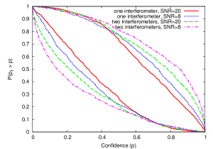
We emphasize that the results discussed so far have made the most pessimistic assumptions about the detector performance, i.e., three months of observation with a single interferometer and $\rho_{\rm thr}=20$. Under such assumptions only a handful of sources will be detected, but this is already sufficient to discriminate among most of the models. In Figures 7 and 8 we consider a specific model comparison (namely VHM-noZ-Edd-co versus VHM-noZ-Edd-ch) to display the effect of relaxing these assumptions.

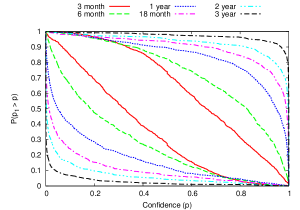
Figure 7 shows that the detector performance does not affect the results substantially. Lowering $\rho_{\rm thr}$ from 20 to 8 for two operational interferometers only adds a few, low SNR, sources to the detected sample, and the gain in discrimination power is limited. On the other hand, Figure 8 shows that the observation duration is crucial. With an observation time of three months, we would achieve a 2$\sigma$ confidence level ($p_{A}=0.95$) with only $\sim 10\%$ probability (i.e., if we repeated an independent 3 month LISA observation $10$ times, we would expect one of these to reach 2$\sigma$ confidence). However, with an observation time of three years, the probability that we will achieve 2$\sigma$ confidence in the underlying model is more than $90\%$ (upper dashed-black curve). There is a similar trend in all model comparisons, although the three month result is particularly bad for this particular comparison, since these models differ only in the accretion geometry which we have seen is the most difficult aspect to distinguish. The trend with observation duration arises simply because the number of detected sources increases linearly with the observation time, and so we have a much better sampling of the underlying model for longer mission durations.

Three-month observation 1 2 3 4 5 6 7 8 9 10 1 $\times$ 0.10 0.72 0.68 0.86 0.88 0.19 0.17 0.91 0.92 2 0.93 $\times$ 0.75 0.69 0.91 0.91 0.17 0.22 0.93 0.93 3 0.42 0.32 $\times$ 0.24 0.45 0.42 0.72 0.69 0.88 0.89 4 0.65 0.63 0.83 $\times$ 0.77 0.76 0.48 0.49 0.80 0.81 5 0.13 0.08 0.58 0.19 $\times$ 0.03 0.93 0.92 0.98 0.99 6 0.12 0.07 0.58 0.21 0.97 $\times$ 0.94 0.92 0.98 0.98 7 0.57 0.57 0.16 0.20 0.05 0.04 $\times$ 0.01 0.93 0.94 8 0.58 0.51 0.16 0.19 0.07 0.07 0.98 $\times$ 0.94 0.95 9 0.16 0.12 0.23 0.31 0.03 0.04 0.17 0.15 $\times$ 0.01 10 0.09 0.07 0.15 0.18 0.02 0.03 0.14 0.13 0.95 $\times$

One-year observation 1 2 3 4 5 6 7 8 9 10 1 $\times$ 0.49 0.99 0.99 1.00 1.00 0.91 0.88 1.00 1.00 2 0.50 $\times$ 0.99 0.99 1.00 1.00 0.92 0.93 1.00 1.00 3 0.00 0.00 $\times$ 0.83 0.97 0.97 1.00 1.00 1.00 1.00 4 0.02 0.02 0.19 $\times$ 0.99 0.99 0.99 0.99 0.99 0.99 5 0.00 0.00 0.03 0.00 $\times$ 0.07 1.00 1.00 1.00 1.00 6 0.00 0.00 0.03 0.00 0.93 $\times$ 1.00 1.00 1.00 1.00 7 0.07 0.06 0.00 0.00 0.00 0.00 $\times$ 0.16 1.00 1.00 8 0.09 0.05 0.00 0.00 0.00 0.00 0.85 $\times$ 1.00 1.00 9 0.00 0.00 0.00 0.01 0.00 0.00 0.00 0.00 $\times$ 0.31 10 0.00 0.00 0.00 0.00 0.00 0.00 0.00 0.00 0.61 $\times$

Table 2: Summary of all possible comparisons of the pure models. The table on the left (right) assumes a LISA observation time of three months (one year), respectively. Models are labeled by an integer $i$, as listed in Table 1. We take a fixed confidence level of $p=0.95$. The numbers in the upper-right half of each table show the fraction of realizations in which the row model will be chosen at more than this confidence level when the row model is true (in the Bayesian figures, this would be the point where a vertical line at $x=p$ intersects the upper curve). The numbers in the lower-left half of each table show the fraction of realizations in which the row model cannot be ruled out at that confidence level when the column model is true (in the Bayesian figures, this would be the point where a vertical line at $x=1-p$ intersects the lower curve). These results are for the pessimistic transfer function ($T_{2}$).

Comparisons between all possible pairs of models are given in Table 2, where we assume a pessimistic detector performance and three months (left) or one year of observation (right), respectively. Even though it is difficult to discriminate among some specific pair of models in the three month observation case, model discrimination is almost perfect in most cases for a one year observation. The exception are the models differing in their accretion geometry only (bold numbers in the table), for which discrimination is difficult. However, even for such similar models we will obtain a high confidence level with probability close to unity if we assume a standard LISA configuration with two operational interferometers observing for three years.

IV Mixed models

In the preceding section we (successfully) demonstrated the potential of LISA to discriminate among a discrete set of “pure” models given a priori. However, the true MBH population in the Universe will probably result from a mixing of the physical processes described in Section II.1, or even from a completely unexplored physical mechanism. It is therefore important to test whether we will be able to extract useful information when the distribution of observed events comes from a mixture of the different models, as an approximation to possible unknowns. For this case study, we will concentrate on the details of the seeding mechanism (mass function and redshift distribution), deferring the more complicated details related to accretion to a future study. Recall in this context that accretion will leave a trace in the spin distribution of MBHs, but our simplified analysis neglects the MBH spins by construction.

We tested two mixing procedures: (i) we generated artificially mixed models that were a linear combination of the pure model distributions presented in Section II.1; (ii) we constructed two consistently mixed models, in which seeds were generated according to a mixing of two prescriptions, and their evolution was followed self-consistently in the halo merger tree realizations. The goal here is to assess whether artificial models can reproduce the salient features of the consistently mixed models, and to estimate the amount of mixing necessary to “best fit” the consistently mixed models. This procedure mimics the analysis of a “real” LISA datastream, for which the data is unlikely to match exactly any one of the pure model predictions.

In this section we describe details of the artificially and consistently mixed models. In Section V that follows we will present the results of the “reconstruction experiment”.

Figure 9: Examples of mixed models. In the upper panels we show marginalized $dN_{i}/dM$ (left) and $dN_{i}/dz$ (right) distributions for the model ${\cal N}$-I (thick solid black lines), in which we mix models VHM-noZ-Edd-co (thin solid red line) and BVR-noZ-Edd-co (thin long-dashed green line). The relative contribution of the models is given by Eq. (19) with $f_{1}=0.23$, $f_{3}=0.77$ (cf. Table 2). In the lower panels we show the same distributions for the model ${\cal N}$-IV (thick solid black lines) in which we mix four “pure” models. The thin lines represent the relative contribution of the individual models VHM-noZ-Edd-co (solid red), VHM-Z-Edd-co (short-dashed blue), BVR-noZ-Edd-co (long-dashed green), and BVR-Z-Edd-co (dot-dashed magenta). The relative contribution of the models is given again by Eq. (19) with $f_{1}=0.08$, $f_{3}=0.22$, $f_{5}=0.56$ and $f_{7}=0.14$ (cf. Table 2).

Artificial mixing simply consists in drawing coalescences from a linear combination of the theoretical coalescence distributions predicted by the pure models. Here, for concreteness, we fix the accretion to be Eddington-limited and coherent, and we mix different seeding recipes. We therefore consider models VHM-noZ-Edd-co, VHM-Z-Edd-co, BVR-noZ-Edd-co, and BVR-Z-Edd-co ($i=1$, $3$, $5$ and $7$ respectively, in the notation of Table 1).

Each model $i$ is characterized by a mean number of predicted coalescences $\bar{N}_{i}$ and a probability distribution for the parameters of the coalescing binaries $p_{i}(M,q,z)$. The predicted event distribution ${\cal N}_{i}=d^{3}N_{i}/dzdMdq$ (see Section II.1) can therefore be factorized as

$${\cal N}_{i}={\bar{N}}_{i}\times p_{i}(M,q,z)\,.$$ (17)

The mixing is described by four parameters $f_{i}$ ($i=1\,,3\,,5\,,7$) which determine the fraction of model $i$ included in the mixed distribution. These fractions are constrained to add up to $1$.

IV.1 Artificial mixing

NAME	Mixing	$f_{1}$	$f_{3}$	$f_{5}$	$f_{7}$	$f_{1}$ fit	$f_{3}$ fit	$f_{5}$ fit	$f_{7}$ fit	$f_{1}+f_{5}$ fit
p-I	$p$	0.15	–	0.85	–	$0.15\pm 0.05$	–	$0.85\pm 0.05$	–	–
p-II	$p$	0.54	–	0.46	–	$0.55\pm 0.1$	–	$0.45\pm 0.1$	–	–
p-III	$p$	0.41	0.13	0.12	0.34	$0.3\pm 0.2$	$0.25\pm 0.25$	$0.1\pm 0.05$	$0.35\pm 0.1$	$0.6\pm 0.05$
p-IV	$p$	0.11	0.49	0.22	0.18	$0.29\pm 0.29$	$0.3\pm 0.3$	$0.21\pm 0.05$	$0.2\pm 0.05$	$0.4\pm 0.05$
${\cal N}$-I	${\cal N}$	0.23	–	0.77	–	$0.2\pm 0.1$	–	$0.8\pm 0.1$	–	–
${\cal N}$-II	${\cal N}$	0.61	–	0.39	–	$0.6\pm 0.15$	–	$0.4\pm 0.15$	–	–
${\cal N}$-III	${\cal N}$	0.31	0.16	0.23	0.3	$0.4\pm 0.2$	$0.1\pm 0.1$	$0.2\pm 0.05$	$0.3\pm 0.05$	$0.5\pm 0.05$
${\cal N}$-IV	${\cal N}$	0.08	0.22	0.56	0.14	$0.15\pm 0.15$	$0.15\pm 0.15$	$0.5\pm 0.1$	$0.2\pm 0.1$	$0.3\pm 0.05$

Table 3: “Artificially mixed” models. Columns 3–6 list the mixing parameters used to generate the models. Columns 7–10 list the best-fit values recovered by our analysis (see Section V).

We tried two different mixing prescriptions. In the first case we ignored the number of coalescences predicted by each specific model, by mixing the respective $p_{i}(M,q,z)$ distributions ($p$ mixing) and normalizing the mixed distribution to some arbitrary number:

$${\cal N}_{p}=\bar{N}_{\rm m}\left\{f_{1}p_{1}+f_{3}p_{3}+f_{5}p_{5}+f_{7}p_{7}\right\},$$ (18)

where $\bar{N}_{\rm m}$ was fixed to 200 coalescences in three years. In the second case we considered the number of predicted events to be an intrinsic property of each individual model, and we simply mixed the $N_{i}(M,q,z)$ distributions (${\cal N}$ mixing) in the same way:

$${\cal N}_{\rm{\cal N}}=f_{1}{\cal N}_{1}+f_{3}{\cal N}_{3}+f_{5}{\cal N}_{5}+f_{7}{\cal N}_{7}\,.$$ (19)

The total number of coalescences is now automatically determined by the values of the mixing parameters. In practice, in order to enforce the constraint that the fractions add up to $1$, we actually use a “nested” prescription based on three parameters $\alpha$, $\beta$ and $\gamma$, which are allowed to take any value in the range $[0,1]$. We then set

$${\cal N}_{\rm{\cal N}}=\alpha{\cal N}_{1}+(1-\alpha)\{\beta{\cal N}_{3}+(1-\beta)[\gamma{\cal N}_{5}+(1-\gamma){\cal N}_{7}]\}\,.$$

We quote our results in terms of the model fractions $f_{i}$, as these are the physically relevant quantities.

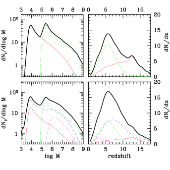
Table 3 lists eight mixed models that we investigated. Examples of ${\cal N}$-mixed model (model ${\cal N}$-I and ${\cal N}$-IV) are also shown in Figure 9. The theoretically observable distributions are generated in the same way as for the pure models, by multiplying the ${\cal N}$ distributions by the appropriate transfer function. Observed datasets ${D_{k}}$ are then generated from the mixed distribution as outlined in Section II.3. Given a dataset ${D_{k}}$, the idea is to parametrize the distribution as a mixture of the available “pure” distributions according to Eqs. (18) or (19), and obtain a posterior distribution for the mixing parameters given the observed data. These posterior distributions allow us to assess which models were mixed, and at what mixing level. To make the test “realistic”, the theoretical mixing and the simulated LISA observations were performed by A. Sesana. The observed datasets ${D_{k}}$ were then analyzed blindly by J. Gair, who did not know which models were mixed nor the amount of mixing.

IV.2 Consistent mixing

We used the consistently mixed models (hybrid models, henceforth labelled “HY”) described in Ref. bv10 . The seeding process was a mixture of the VHM-Z and BVR-Z mechanisms, and the MBH mass growth assumed Eddington limited, coherent accretion. We considered two models with fixed POPIII seeding efficiency, but different quasistar seeding efficiencies. The quasistar seeding efficiency is related to the maximum halo spin parameter, $\lambda$, that allows efficient transfer of gas to the center to form a quasistar (see Ref. bv10 for details). We test an inefficient quasistar seeding model ($\lambda=0.01$, HY-I) and an efficient quasistar seeding model ($\lambda=0.02$, HY-II) that predict MBH population observables (local mass function, quasar luminosity function, and so on) bracketing the current range of allowed values.

To check the effectiveness of our analysis tools in extracting information about the parent MBH population, we try to recover the hybrid model distributions as a mixing of the VHM-Z and BVR-Z “pure” models, of the form given by either Eq. (18) or (19). The procedure is the same as detailed in the previous section.

Let us stress again that the MBH evolution through cosmic history is followed self-consistently in the hybrid models. This means that the predicted theoretical distribution is not, in general, described as a simple mixing of the form given by Eqs. (18) or (19). This is a crucial point: the success of this experiment will tell us that we can extract valuable information on complex MBH formation scenarios by mixing a set of “pure” models based on simple recipes.

Figure 10: Summary of the model mixing results for models ${\cal N}$-I and ${\cal N}$-II. In both panels, the horizontal axis shows the mixing fraction for model VHM-noZ-Edd-co. The left panel shows the posterior probability distribution function for this mixing fraction as found in one particular realization of each model. The right panel shows how the peak of the posterior was distributed over 100 different realizations of each of the two models. The vertical lines show the true values of the mixing fraction.

Figure 11: Summary of model mixing results for model ${\cal N}$-III. We show the mixing fraction of the given model on the horizontal axis. The left panel shows the posterior probability distribution of the mixing fraction for each of the four models, VHM, BVR, VHM-Z and BVR-Z, found when analyzing a single realization of model ${\cal N}$-III. The central panel shows the same thing, but now considering the fractions of BVR, BVR-Z and the sum VHM+VHM-Z in the mixed model. The right panel shows the distribution of the peak of the posterior pdf found over 100 different realizations of the ${\cal N}$-III model.

V Results for the mixed models

In the context of mixed models, we are no longer comparing two pre-assigned models A and B as descriptions of the observational data. We deal instead with a single, continuous parameter space of models, where the parameters are the mixing fractions of some subset of “pure” models. For example, if we mix models 1 and 3, we have a one-dimensional parameter space given by the contribution of model 1 ($f_{1}$) to the total population (the contribution of model 3 is fixed by the constraint $f_{1}+f_{3}=1$). Given a particular observation, we can then compute the posterior probability distribution function (PDF) given by Bayes theorem, Eq. (12), for the mixing fractions. The computation of the posterior can be done either over a grid of points in the parameter space, or by exploring the parameter space by means of Markov Chain Monte Carlo simulations (which become much more practical as the dimension of the parameter space increases).

For each mixed model, 100 different realizations of the LISA data were generated and a posterior probability distribution for the mixing fractions was obtained for each one. The width of the posterior in a single realization reflects how well that particular data set can constrain the mixing fractions. The location of the peak of the posterior will change from realization to realization, but we would expect the width to remain approximately the same. We also expect that the distribution of the location of the peak of the posterior over many realizations should resemble the posterior for the mixing fractions computed in any single realization.

We considered a total of eight different mixed models, as listed in Table 3, mixing either just VHM-noZ-Edd-co and BVR-noZ-Edd-co or these two models plus VHM-Z-Edd-co and BVR-Z-Edd-co. For each case, we assumed that we were using three years of LISA data, but made pessimistic assumptions ($T_{2}$) for the transfer function. While this latter assumption is slightly conservative, we checked that there was not much difference in performance when using the most optimistic assumptions (i.e., the transfer function $T_{3}$).

Figure 12: Two-dimensional marginalized posterior PDFs obtained from a single realization of model ${\cal N}$-III. Each plot shows the mixing fraction of one model component against the mixing fraction of a second component. The models are numbered from $1$, $3$, $5$ and $7$, corresponding to VHM, VHM-Z, BVR and BVR-Z respectively, as in Table 1. The top row shows comparisons between model 1 (horizontally) and models 3, 5 and 7, respectively. The bottom row shows comparisons 3 to 5, 3 to 7 and 5 to 7, respectively. Note that the individual components of VHM and VHM-Z are poorly constrained, which is why the plots involving VHM models have larger correlation contours than the BVR to BVR-Z comparison (bottom right).

Figure 13: Comparison of intrinsic and “recovered” distributions for the consistently mixed models. In each panel, the thick solid black curve shows the intrinsic distribution of mergers in the model, the red solid line shows the “recovered” distribution, which is a sum of the VHM-Z and BVR-Z models, weighted by the best-fit mixing parameter. The thin lines show the contributions to this recovered distribution from the VHM-Z (solid blue) and BVR-Z (dashed magenta) models. The left panels show the distributions of the masses of mergers, while the right panels show the distributions of the redshifts of mergers. The upper panels show the distribution for observed merger events, while the lower panels show the intrinsic distribution of mergers.

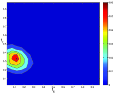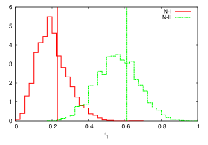
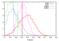
The posterior distributions of the mixing fraction found in one particular realization each of models ${\cal N}$-I and ${\cal N}$-II are shown in the left panel of Figure 10. The PDFs peak around $f_{1}=0.2\pm 0.05$ for model ${\cal N}$-I and $f_{1}=0.55\pm 0.1$ for model ${\cal N}$-II, which is consistent with the injected fractions listed in Table 3.

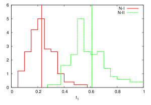
As mentioned above, we expect the peak and width of the posterior PDF to fluctuate from realization to realization. To assess the statistical robustness of this result we therefore repeat the experiment. In the right panel of Figure 10, we plot the distribution of the location of the peak of the posterior PDF found in each of 100 realizations of the models. As we expect, the widths of these distributions are very similar to the PDFs found in each of the individual realizations. The distribution peaks around $f_{1}=0.2\pm 0.05$ for model ${\cal N}$-I and around $f_{1}=0.55\pm 0.1$ for model ${\cal N}$-II, in agreement with the true injected fractions listed in Table 3. This experiment shows that most of the time we can correctly infer the relative contribution of the two models, but there is still the possibility to draw erroneous conclusions from a single observation. For example, in two realizations of model ${\cal N}$-II we would prefer an almost pure VHM model, while the underlying distribution is in fact 45% BVR. However, in these cases the posterior PDF is also very wide, which would be an indicator that the data set was not placing particularly good constraints on the model in that specific case.

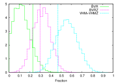
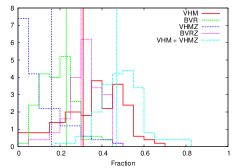
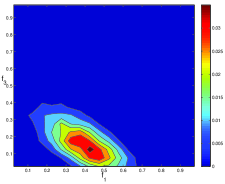
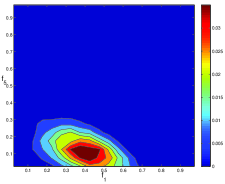
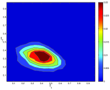
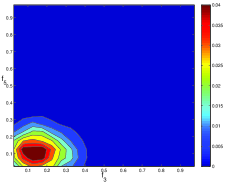
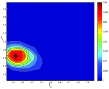
Figure 11 shows the results for the more complex case of model ${\cal N}$-III, where all four of the pure models were mixed and the mixing parameter space is three dimensional. Again, both the posterior PDFs given by a specific realization (left panel) and the distribution of the peak values of the posterior PDFs in a sample of 100 realizations return mixing fractions which are consistent with the injected values (see Table 3). However, in this case the width of the VHM-noZ and VHM-Z posterior PDFs is large ($\sim 0.2$), indicating a certain degree of degeneracy between those two models. If we consider the sum, then the posterior PDF is much narrower and peaks at the right value ($f_{1}+f_{5}=0.47$, see Table 3), showing that there is much less degeneracy between the VHM and the BVR models. This is also nicely shown by the two dimensional posterior PDFs plotted in Figure 12. All the ellipse contours have principal axes more or less directed along the $x$ and $y$ axes, with the exception of the VHM-noZ versus VHM-Z PDF, which shows a clear anticorrelation between those two fractions.

Although we focused on the ${\cal N}$ models, the same level of accuracy in the determination of the mixing fractions is achieved for $p$ models. The results are collected in Table 3. The results shown in the table refer to the most pessimistic transfer function; slightly better constraints on the mixing fractions can be obtained if we assume two operational interferometers and $\rho_{\rm thr}=8$.

As a final step we present our results for the consistent mixing model. In the two hybrid models HY-I and HY-II, VHM-Z and BVR-Z seeding prescriptions are simultaneously employed in a consistent way in the merger trees, and we do not expect the resulting binary population to be perfectly reproduced by any combination of our pure models. The test here is to combine the two “pure” VHM-Z ($i=3$) and BVR-Z ($i=7$) models to see if we can mimic the true distribution with some combination of the two. We proceed exactly as for the artificial mixing, by recovering the posterior PDF of the mixing parameter. In this case we used only the $p$-type mixing model, and included maginalization over the total number of events as given by Eq. (16). The rationale for this was that we thought a consistent mixed model of this type would not necessarily have the same number of events as the underlying models, and so we wanted to eliminate bias that would be introduced by using the number-of-event information. We also computed results using the ${\cal N}$-type mixing and/or not marginalizing over the number. These results were also reasonable, but the match between the intrinsic and recovered distributions was not as good.

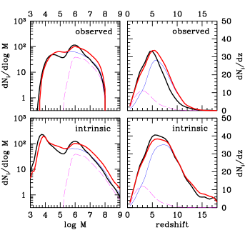
For $p$-type mixing with marginalization over number, we find that model HY-I and HY-II are best reproduced by setting $f_{3}=0.85$ and $f_{3}=0.45$, respectively. The marginalized mass and redshift distributions of the best-fitting model are shown as red lines for model HY-I in Figure 13. As expected, we can not perfectly match the true model distribution, but the overall agreement is good. Even though there is no “true answer” in this case, we can still extract useful information about the models. For example, we can confidently say that in model HY-II the contribution of the heavy seeding process is much higher than in model HY-I. This is consistent with the fact that model HY-II assumes a much more efficient quasistar formation prescription.

VI Conclusions

In this paper we explored the “inverse problem” for GW observations, which is fundamental in assessing the possible astrophysical impact of GW astronomy. The question we addressed in this paper was: given a sample of observed MBHB coalescences (with relative parameter estimation errors), what astrophysical information about the physical processes governing their formation and cosmological evolution can we extract from the observations? More informally: are GW observations a valuable tool for astrophysics? We answered this question by applying the statistical framework of Bayesian model selection to simulated LISA observed datasets. We chose LISA as a case study, but the analysis could straightforwardly be generalized to any other GW detector.

We considered ten different “pure” MBH formation and evolution models (see Table 1) differing in certain key aspects of the input physics, specifically: (i) the seed formation mechanism, (ii) the redshift distribution of the first seeds, (iii) the accretion efficiency during each merger and (iv) the geometry of accretion (see Section II.1). For each model we computed the intrinsic coalescence distributions $d^{3}N_{i}/dMdqdz$. We then constructed the theoretically observable distributions by filtering the intrinsic distributions with four transfer functions $T_{j}$. These transfer functions account for different levels of completeness of the LISA observations according to four different sets of assumption about the performance of the LISA detector (Section II.2). For each model we generated 1000 observed datasets (including observational errors), and we analyzed them using a Bayesian model selection framework to assess their distinguishability as a function of the detector performance and of the duration of the dataset used for the model comparison. We find that:

• LISA will be able to discriminate among almost any pair of such “pure” models, even under pessimistic assumptions about the detector performance, after only one year of operation (see Table 2). In particular, it will be easy to identify the mass and redshift distribution of the seeds, and the efficiency of the accretion mechanism.

• Models differing only by their accretion geometry are more difficult to discriminate. However, this was partly a consequence of our choice to consider measurements of only three parameters for each inspiralling binary (mass, mass ratio and redshift), i.e., we ignored the information encoded by MBH spins and in the merger/ringdown. Including spins in the analysis will probably make such models easily distinguishable, as demonstrated in a similar study by Plowman et al.  plowman10 . In any case, even without the extra information carried by the spins, we can discriminate between these models if we consider the optimal LISA performance and three years of observation.

• The impact of the detector performance on the analysis is relatively mild. This is because lowering the threshold to $\rho_{\rm thr}=8$ and considering two interferometers only adds a small number of sources to the detected sample, and only slightly improves parameter estimation.

• Not surprisingly, the length of the observation is important, as the expected number of MBHBs in the sample increases linearly with the observation time. To give a specific figure of merit, with a three-year observation window we have more than a $90\%$ probability that the parent model of an observed sample will be safely identified at a two-sigma confidence level (95%).

To go beyond the pure model analysis, we considered the possibility of model mixing. First we created new, “artificial” models by mixing the coalescence distribution functions of different “pure” models (namely, models 1, 3, 5 and 7, see Tables 1 and 3). We used pure models differing in their seeding mechanism and in the redshift distribution of the seeds (different metallicity “feedback”). The new models are characterized by the fractions $f_{i}$ of the “pure” models used in the mixing, with the constraint $\sum_{i}f_{i}=1$. Then we considered two hybrid models, where halos were simultaneously seeded according to the VHM-Z ($i=3$) and the BVR-Z ($i=7$) prescription, and the evolution of the seeds was self-consistently followed in the halo hierarchy. We produced several LISA observed datasets for both the artificial and the hybrid models. We then tried to recover the combination of “pure” models that best reproduces each mixed model by maximizing over the posterior probability distribution function of the likelihood (Section V). We find that:

• When the “pure” models used in the mixing differ only in their seeding prescription (VHM vs BVR), so that we have only a single mixing parameter (since $\sum_{i}f_{i}=1$), we can correctly infer this mixing parameter with an accuracy of about $10\%$.

• When we mix four different models we can still infer the mixing fractions with the same accuracy, but there is a certain degree of degeneracy between the two VHM models ($i=1$ and $i=5$); i.e., the effect of metallicity “feedback”, as the detectable MBH population does not differ much between these two models. However, the fraction $f_{1}+f_{5}$ is very well constrained, and we can clearly distinguish the relative contribution from the different seeding mechanisms.

• Finally, we can also get a fairly good match to the hybrid models by combining “pure” models. This is probably the most important result of our analysis. The formation and merger history of MBHs is a complex process, involving several physical ingredients which are poorly understood, and it is difficult to imagine that we will have a comprehensive theoretical understanding of the underlying physics before LISA flies. However, we will certainly be able to construct a set of models based on simple physical prescriptions that can be tested against the observations. Our experiment with the hybrid models demonstrates that we can extract valuable information about more complex MBH formation scenarios by mixing a set of “pure” models based on simple recipes.

The use of a Bayesian framework is crucial for the model mixing results, since it allows us to recover a posterior probability distribution for the “mixing parameters” that characterizes the fraction of each model contributing to the observed data set. In this respect, our analysis goes considerably beyond the work recently presented in Ref. plowman10 , where only pure models were considered and the statistical analysis was based on two dimensional Kolmogorov-Smirnov tests performed on the distributions of pairs of measured parameters.

Despite this improvement, the building blocks of the present work can be improved in many ways. The set of distinct “pure” models can not be representative of all the physical complexity of the problem. A more powerful approach to MBH population modelling would be to describe the relevant physics using a set of continuous parameters representing the critical features of the models (seed mass function, accretion efficiency and so on), and then attempt to measure those parameters by performing a similar Bayesian analysis. We have also adopted several simplifying assumptions about the GW observations, which can be refined by developing a more realistic model for the GW signal, including spins, higher harmonics, merger and ringdown. We can then attempt a more sophisticated analysis and explore the posterior probability distribution function in a larger and more complex parameter space, to maximize the recovered information. All these issues should be explored in the future.

Besides the scientific impact of a GW detection in and by itself, the ambitious goal of doing GW astronomy requires that we maximize the astrophysical information that will be extracted from such detections. In this respect, addressing the “inverse problem” in GW astronomy is extremely important. In this paper we have made a first, small step in this direction. We hope that our work will encourage relativists and GW astronomers to consider in greater depth the astrophysical impact of GW detections. At the same time, we hope to convince “ordinary” astronomers that GWs can be an important tool, not only for tests of general relativity and as a laboratory for fundamental physics, but also in astrophysics.

Appendix A Error modelling

We describe here how measurement errors are included in the analysis. Errors arise due to instrumental noise in the LISA detector, and from the transformation between different coordinates. The error propagation expressions described below are probably not new, and the end result is expected, but we include the derivation here for completeness and to clarify the underlying assumptions.

LISA observations will determine the luminosity distance to a given source, but we want to characterize the source by the redshift instead. The conversion can be done using the concordance cosmology at the time LISA flies, but this introduces additional errors, since the cosmological parameters will be known imperfectly. Suppose we want parameters $\vec{x}$ which are given by the measured parameters, $\vec{y}$, and a transformation $\vec{x}(\vec{y};\vec{\lambda})$ that depends on some imperfectly known parameters, $\vec{\lambda}$. Suppose further that the probability distribution for $\vec{\lambda}$ is $L(\vec{\lambda})$ and that for $\vec{y}$ is $Y(\vec{y})$. The probability distribution for $\vec{x}$ is then

$$X(\vec{x})=\int L(\vec{\lambda})Y(\vec{y}(\vec{x};\vec{\lambda}))J(\vec{x};\lambda){\rm d}^{n_{\lambda}}\lambda\,,$$ (20)

in which $J(\vec{x};\lambda)$ is the Jacobian for the transformation between $\vec{y}$ and $\vec{x}$ and $n_{\lambda}$ is the dimensionality of the $\vec{\lambda}$ parameter space. We now make two simplifying assumptions: (i) the distributions of the errors in $\vec{y}$ and $\vec{\lambda}$ are multi-variate Gaussians with inverse variance-covariance matrices $\Gamma^{y}$ and $\Gamma^{\lambda}$ respectively; (ii) the errors are small, so that the distributions are peaked near the true values of $\vec{y}_{0}$ and $\lambda_{0}$. This latter assumption means that we can use a linear approximation in the interesting region of the distributions

$$y_{i}(\vec{x};\vec{\lambda})\approx y_{i}(\vec{x}_{0};\lambda_{0})+\frac{\partial y_{i}}{\partial x_{j}}(x_{j}-x_{0j})+\frac{\partial y_{i}}{\partial\lambda_{j}}(\lambda_{j}-\lambda_{0j})\,,$$ (21)

where the derivatives are evaluated at $\vec{y}_{0}$, $\vec{\lambda}_{0}$. We can also ignore the Jacobian in the integrand of Eq. (20), since it will be approximately constant across the domain of integration and therefore it plays the role of a normalization factor. Using the notation

$$\tilde{x}_{i}=x_{i}-x_{0i},\;\;\delta{\lambda}_{i}=\lambda_{i}-\lambda_{0i},\;\;D^{x}_{ij}=\frac{\partial y_{i}}{\partial x_{j}},\;\;D^{\lambda}_{ij}=\frac{\partial y_{i}}{\partial\lambda_{j}}\,,$$ (22)

we see that the integrand is proportional to the exponential of

$$-\frac{1}{2} \left\{\left((D^{x}{\bf\tilde{x}})^{T}+\delta{\bf\lambda}^{T}D^{\lambda}\right)\Gamma^{y}\left(D^{x}{\bf\tilde{x}}+(D^{\lambda})^{T}\delta{\bf\lambda}\right)\right.$$ (23)

$$\left.+\delta{\bf\lambda}^{T}\Gamma^{\lambda}\delta{\bf\lambda}\right\}\,,$$

where matrix notation is being used. This can be rearranged to give

$$-\frac{1}{2} \left\{(D^{x}{\bf\tilde{x}})^{T}\Gamma^{y}D^{x}{\bf\tilde{x}}-{\bf a}^{T}(\Gamma^{\lambda}+D^{\lambda}\Gamma^{y}(D^{\lambda})^{T}{\bf a}\right.$$ (24)

$$\left.+\left(\delta{\bf\lambda}+{\bf a}\right)^{T}\left(\Gamma^{\lambda}+D^{\lambda}\Gamma^{y}(D^{\lambda})^{T}\right)\left(\delta{\bf\lambda}+{\bf a}\right)\right\}\,,$$

where

$${\bf a}=\left(\Gamma^{\lambda}+D^{\lambda}\Gamma^{y}(D^{\lambda})^{T}\right)^{-1}D^{\lambda}\Gamma^{y}D^{x}{\bf\tilde{x}}\,.$$ (25)

The term on the second line of Eq. (24) is just a Gaussian, whose centre has been shifted to ${\bf a}$, and with variance-covariance matrix that is independent of ${\bf\tilde{x}}$. When we integrate over the distribution of $\vec{\lambda}$, i.e., over $\delta{\bf\lambda}$, we find the probability distribution is proportional to the exponential of

$$-\frac{1}{2}\left\{(D^{x}{\bf x})^{T}\Gamma^{y}D^{x}{\bf x}-{\bf a}^{T}(\Gamma^{\lambda}+D^{\lambda}\Gamma^{y}(D^{\lambda})^{T}{\bf a}\right\}\,,$$ (26)

which is a multi-variate Gaussian with variance-covariance matrix $\Gamma^{x}$ equal to

$$(D^{x})^{T}\left(\Gamma^{y}-\Gamma^{y}(D^{\lambda})^{T}\left(\Gamma^{\lambda}+D^{\lambda}\Gamma^{y}(D^{\lambda})^{T}\right)^{-1}D^{\lambda}\Gamma^{y}\right)D^{x}.$$ (27)

Although this expression looks complicated, the inverse of this matrix takes the simple form

$$(\Gamma^{x})^{-1}=(D^{x})^{-1}\left((\Gamma^{y})^{-1}+(D^{\lambda})^{T}(\Gamma^{\lambda})^{-1}D^{\lambda}\right)((D^{x})^{T})^{-1}.$$ (28)

As it is this inverse matrix which determines the width of the distributions, we see that it takes the form we might expect, i.e., the error is the sum of the error contributions from the instrumental noise, $\Gamma^{y}$, and that from the uncertainty in the cosmological parameters, $\Gamma^{\lambda}$. The remaining terms just propagate the errors through the transformation in the standard way.

In this paper, we estimate the errors in the observed parameters, $\Gamma^{y}$, using the Fisher matrix formalism of Ref. Berti:2004bd . These errors are given in terms of the chirp mass, ${\cal M}$, the amplitude, $A$, and the symmetric mass ratio, $\eta$, so we must transform these coordinates to mass, $M$, luminosity distance, $D_{L}$, and mass ratio, $q$. We convert luminosity distance to redshift by inverting the standard cosmological relation of Eq. (9). We assume that there are errors in $H_{0}$ and $\Omega_{\Lambda}$ but enforce flatness (i.e., $\Omega_{M}+\Omega_{\Lambda}=1$).

The diagonal components of the total error matrix in the new variables, $(\Gamma^{x})^{-1}$, are then

$$\left(\Gamma^{x}\right)^{-1}_{\ln q\ln q} = \frac{1}{1-4\eta}\left(\Gamma^{y}\right)^{-1}_{\ln\eta\ln\eta}\,,$$

$$\left(\Gamma^{x}\right)^{-1}_{\ln M\ln M} = \left(\Gamma^{y}\right)^{-1}_{\ln{\cal M}\ln{\cal M}}+\frac{9}{25}\left(\Gamma^{y}\right)^{-1}_{\ln\eta\ln\eta}$$

$$-\frac{6}{5}\left(\Gamma^{y}\right)^{-1}_{\ln{\cal M}\ln\eta},$$

$$\left(\Gamma^{x}\right)^{-1}_{zz} = \left(\frac{\partial D_{L}}{\partial z}\right)^{-2}\left[D_{L}^{2}\left(\frac{5}{6}\left(\Gamma^{y}\right)^{-1}_{\ln{\cal M}\ln{\cal M}}\right.\right.$$ (29)

$$+\left(\Gamma^{y}\right)^{-1}_{\ln A\ln A}+\frac{5}{3}\left(\Gamma^{y}\right)^{-1}_{\ln{\cal M}\ln A}$$

$$\left.\left.+\frac{\Delta H_{0}^{2}}{H_{0}^{2}}\right)+\Delta\Omega_{\Lambda}^{2}\left(\frac{\partial D_{L}}{\partial\Omega_{\Lambda}}\right)\right].$$

where $(\Gamma^{y})^{-1}_{ij}$ denotes the components of the inverse Fisher matrix as given in Ref. Berti:2004bd , and $\Delta H_{0}$, $\Delta\Omega_{\Lambda}$ are the errors in the cosmological parameters at the time of the LISA mission, which we take to be $\Delta H_{0}/H_{0}=\Delta\Omega_{\Lambda}/\Omega_{\Lambda}=0.01$. The off-diagonal components in the total error matrix come only from the rotation of the noise error matrix, $(D^{x})^{-1}(\Gamma^{y})^{-1}((D^{x})^{T})^{-1}$, but in practice we ignore these and draw errors based on the diagonal variance-covariance matrix with components as above. This is conservative, in that it approximates the error ellipse by a bounding circle, but we have also checked that our results did not significantly change when they were recomputed using the full error model including correlations.

Figure 14: SNR contours in the $(M\,,q)$ plane at different redshifts (from left to right: $z=0.5\,,5$ and $20$). The top row refers to the averaged code, the bottom row to the Cutler code with $T_{\rm obs}=3$ yrs and two interferometers.

We note that there is a singularity in the transformation between $\eta$ and $q$ when $q=1$ ($\eta=0.25$, which is indicated by the divergence of $\left(\Gamma^{x}\right)^{-1}_{qq}$ there). The probability that two galaxies with exactly the same black hole mass merge is zero, and so this was not a problem in practice.

Additional errors arise from the effects of weak lensing. This means that the apparent luminosity distance, $d_{A}$, of a source at the Earth is changed by a factor $\mu$ from the true luminosity distance, $d_{T}$, so that $d_{A}=\mu d_{T}$. If we assume that the weak-lensing (de-)magnification is drawn from a Gaussian distribution (which is a reasonable approximation in the weak-lensing limit, although not for stronger lensing), we can use the preceding arguments in this case as well. The parameters $\vec{x}$ are the parameters we assign to the source, which are the same as the measured parameters $\vec{y}$. However, for a fixed value of $\mu$, the distribution of $\vec{y}$ is centred at a luminosity distance $\mu d_{T}$. When we marginalize over possible values of $\mu$, we end up with an integral of the form (20), but the dependence of the integrand on the unknown parameter is through the centre of the distribution, $\vec{y}_{0}$, rather than through the mapping to $\vec{x}$. We can follow the same arguments as before, but replace the derivatives in equation (21) by derivatives of $\vec{y}-\vec{y}_{0}$. The end result then takes the same form. If the distribution of $\mu$ is a Gaussian $\exp(-\Gamma_{\mu\mu}(\mu-1)^{2}/2)$, we find the $(\Gamma^{x})^{-1}_{dd}$ component must be corrected by addition of $d_{T}^{2}/\Gamma_{\mu\mu}$. In practice, we take the weak-lensing error estimate $\Delta z_{\rm wl}$ from Ref. wangholz , and directly modify the $zz$ component as $(\Gamma^{-1})_{zz}\rightarrow(\Gamma^{-1})_{zz}+(\Delta z_{\rm wl})^{2}$.

While we formulated the above in terms of computing the distribution of errors in the parameters we measure from our observation, the same framework can be applied to the analysis of the real LISA data set. Once we obtain a posterior PDF for the measured waveform parameters, $Y(\vec{y})$, we can combine this with a posterior on the cosmological parameters and on the lensing magnification distribution through Eq. (20) to derive the posterior on the inferred source parameters $\vec{x}$. With the assumption that these measured posteriors are Gaussians, the final result will take the same form.

Appendix B Effect of LISA motion on SNR and estimation of intrinsic parameters

Figure 15: Contours of the error on the chirp mass in the $(M\,,q)$ plane at different redshifts (from left to right: $z=0.5\,,5$ and $20$). The top row refers to the averaged code, the bottom row to the Cutler code with $T_{\rm obs}=3$ yrs and two interferometers.

In this paper we tried to provide conservative estimates of the astrophysical potential of LISA through observing MBH binaries. For this reason we only considered MBHB inspiral waveforms in the restricted post-Newtonian approximation. The choice of simple, frequency-domain waveforms has the advantage that it significantly speeds up parameter estimation calculations: we can easily compute the SNR and parameter estimation accuracy of $\sim 10^{6}$ binaries in one day on a single processor, something that would be impossible if we used time-domain waveforms including spin precession. Computational requirements were indeed a limiting factor in the analysis by Plowman et al. plowman10 , who used an advanced parameter estimation code developed by the Montana group Arun:2008zn .

In Ref. Berti:2004bd , the potential of LISA to estimate binary parameters was assessed using two independent formalisms. In one case (“non angle-averaged”) the motion of LISA was taken into account using the formalism developed by Cutler Cutler:1997ta ; in the other case (“angle-averaged”) the authors averaged over the LISA beam-pattern functions. The angle-averaging procedure removes all information related to the Doppler shift due to the motion of LISA around the Sun, so in the angle-averaged formalism it is impossible to estimate the distance and angular location of the source in the sky. However, it is still possible to obtain an “angle-averaged” estimate of the SNR and of the intrinsic parameters of the source (for our nonspinning binary model there are only two of them: $M$ and $q$, or equivalently, ${\cal M}$ and $\eta$).

In summary, there are two ways of assessing the parameter estimation capabilities of LISA. In the first method we angle-average over pattern functions, then we estimate the SNR and the accuracy in determining (say) ${\cal M}$ and $\eta$. In the second method we perform a Monte Carlo sampling of the pattern function (by assuming that the source location and angular orientation in the sky are isotropically distributed). In this way we can estimate the SNR of each source, as well as the accuracy in determining (say) ${\cal M}$, $\eta$, the luminosity distance $D_{L}$ and the angular position of the source $\Delta\Omega$.

In this Appendix we address the question: when these two procedures can be compared at all (i.e., in the case of ${\cal M}$, $\eta$ and the SNR), how are they related? If the angle-average over pattern functions provides a sensible estimate of SNRs and of the intrinsic binary parameters, it could provide a significant saving in terms of computational time for future studies of MBH populations.

In Figure 14 we show contour plots of the SNR in the $(M\,,q)$ plane at selected values of the redshift, for both the averaged and the non-averaged cases. This plot is encouraging: it shows that the shape of these contour plots is essentially identical. Indeed, a more careful analysis reveals that the ratio between the averaged and non-averaged SNRs is SNR_A/SNR${}_{\rm NA}\simeq 1.3$ and it is (to a very good approximation) independent of $(M\,,q\,,z)$.

Fisher matrix calculations are inaccurate when the SNR is not much larger than unity (see e.g. Vallisneri:2007ev ). Figure 14 can be used to identify regions where the SNR becomes so small that the Fisher matrix approach will fail, and other parameter estimation techniques (such as Markov Chain Monte Carlo) will become necessary. For example, by looking at the contour line with SNR $\rho=8$ we see that Markov Chain Monte Carlo calculations will be necessary to estimate the parameter estimation errors for mergers of low-mass black holes at high redshift. In this context, recall that $M=(1+z)M_{r}$, so (for large redshifts) the total mass in the source frame $M_{r}$ is smaller than the mass $M$ appearing on the $y$ axis of the contour plots.

Can we find more empirical relations between the pattern-averaged formalism and the Cutler approach? Figure 15 shows contour plots of the chirp mass determination accuracy in the two formalisms. Once again, we see that there is indeed an approximate proportionality between mass estimation accuracies in the two approaches. The ratios of the chirp mass errors show small random fluctuations consistent with the Poisson noise in the $10^{3}$ Monte Carlo realizations at each point, but it is clear that the angle-averaged approach does a good job at predicting the SNR and the intrinsic parameter errors. This is true at any redshift. Indeed, we find that ratios in the errors on ${\cal M}$ and $\eta$ are pretty much redshift independent, and they show a very mild variation (in the range $\sim 1-1.2$) in the $(M\,,q)$ plane. If a similar proportionality applies also to estimates of the MBH spins, the pattern-averaging may turn out to be a very useful simplication for future MBH population studies.

Figure 16: Contours of the angular resolution error in the $(M\,,q)$ plane at different redshifts (from left to right and from top to bottom: $z=0.5\,,2\,,20$). The calculation uses Cutler’s formalism with $T_{\rm obs}=3$ yrs and two interferometers.

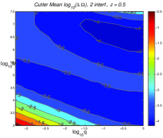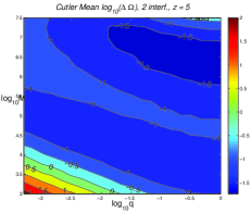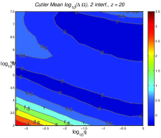To finish, we will point out an interesting trend in the expected accuracy of angular resolution. We are not aware of systematic calculations of the angular resolution in the three dimensional $(M\,,q\,,z)$ parameter space, so we present such a study in Figure 16. Angular resolution degrades with redshift, as expected. The plot shows that, for any given redshift, the angular resolution accuracy has a bimodal distribution – i.e., there are two islands of good angular resolution accuracy in the $(M\,,q)$ plane. In hindsight, this is not too surprising: the “lower” island corresponds to low-mass binaries from which the GW emission is in the optimal sensitivity bucket of LISA; the “upper” island correspond to higher-mass binaries that merge at lower frequency, but have SNR large enough to compensate for the relatively small number of cycles spent in band. It will be interesting to verify if such a bimodal distribution persists when the merger/ringdown signal is also included in the analysis.

References

- (1) S. D. M. White and M. J. Rees, Mon. Not. Roy. Astron. Soc. 183, 341 (1978).
- (2) G. Kauffmann and M. Haehnelt, Mon. Not. Roy. Astron. Soc. 311, 576 (2000), [arXiv:astro-ph/9906493].
- (3) M. Volonteri, F. Haardt and P. Madau, Astrophys. J. 582, 559 (2003), [arXiv:astro-ph/0207276].
- (4) Z. Haiman and K. Menou, ApJ 531, 42 (2000).
- (5) G. Kauffmann and M. Haehnelt, MNRAS 311, 576 (2000).
- (6) J. S. B. Wyithe and A. Loeb, ApJ 595, 614 (2003).
- (7) D. J. Croton et al., MNRAS 356, 1155 (2005), [astro-ph/0407537].
- (8) R. K. Malbon, C. M. Baugh, C. S. Frenk and C. G. Lacey, Mon. Not. Roy. Astron. Soc. 382, 1394 (2007), [arXiv:astro-ph/0607424].
- (9) T. Di Matteo, J. Colberg, V. Springel, L. Hernquist and D. Sijacki, ApJ 676, 33 (2008), [arXiv:0705.2269].
- (10) J. Magorrian et al., Astron. J. 115, 2285 (1998), [arXiv:astro-ph/9708072].
- (11) S. Gillessen et al., Astrophys. J. Lett.707, L114 (2009), [0910.3069].
- (12) S. A. Hughes, Mon. Not. Roy. Astron. Soc. 331, 805 (2002), [astro-ph/0108483].
- (13) K. G. Arun et al., Class. Quant. Grav. 26, 094027 (2009), [0811.1011].
- (14) E. Berti, V. Cardoso and C. M. Will, Phys. Rev. D73, 064030 (2006), [gr-qc/0512160].
- (15) S. T. McWilliams, J. I. Thorpe, J. G. Baker and B. J. Kelly, Phys. Rev. D81, 064014 (2010), [0911.1078].
- (16) D. E. Holz and S. A. Hughes, Astrophys. J. 629, 15 (2005), [astro-ph/0504616].
- (17) K. G. Arun, B. R. Iyer, B. S. Sathyaprakash, S. Sinha and C. V. D. Broeck, Phys. Rev. D76, 104016 (2007), [0707.3920].
- (18) C. Van Den Broeck, M. Trias, B. S. Sathyaprakash and A. M. Sintes, Phys. Rev. D81, 124031 (2010), [1001.3099].
- (19) S. Hilbert, J. R. Gair and L. J. King, 1007.2468.
- (20) S. Babak, J. R. Gair, A. Petiteau and A. Sesana, 1011.2062.
- (21) S. M. Koushiappas, J. S. Bullock and A. Dekel, Mon. Not. Roy. Astron. Soc. 354, 292 (2004), [arXiv:astro-ph/0311487].
- (22) G. Lodato and P. Natarajan, Mon. Not. Roy. Astron. Soc. 371, 1813 (2006), [arXiv:astro-ph/0606159].
- (23) M. C. Begelman, M. Volonteri and M. J. Rees, Mon. Not. Roy. Astron. Soc. 370, 289 (2006), [arXiv:astro-ph/0602363].
- (24) M. Volonteri and M. C. Begelman, ArXiv e-prints (2010), [1003.5220].
- (25) J. S. B. Wyithe and A. Loeb, Astrophys. J. 590, 691 (2003), [arXiv:astro-ph/0211556].
- (26) A. Sesana, F. Haardt, P. Madau and M. Volonteri, Astrophys. J. 611, 623 (2004), [arXiv:astro-ph/0401543].
- (27) A. Sesana, F. Haardt, P. Madau and M. Volonteri, Astrophys. J. 623, 23 (2005), [arXiv:astro-ph/0409255].
- (28) A. Sesana, M. Volonteri and F. Haardt, Mon. Not. Roy. Astron. Soc. 377, 1711 (2007), [arXiv:astro-ph/0701556].
- (29) M. Enoki, K. T. Inoue, M. Nagashima and N. Sugiyama, Astrophys. J. 615, 19 (2004), [arXiv:astro-ph/0404389].
- (30) K. J. Rhook and J. S. B. Wyithe, Mon. Not. Roy. Astron. Soc. 361, 1145 (2005), [arXiv:astro-ph/0503210].
- (31) J. E. Plowman, D. C. Jacobs, R. W. Hellings, S. L. Larson and S. Tsuruta, Mon. Not. Roy. Astron. Soc. 401, 2706 (2010), [0903.2059].
- (32) J. E. Plowman, R. W. Hellings and S. Tsuruta, ArXiv e-prints (2010), [1009.0765].
- (33) J. R. Gair, A. Sesana, E. Berti and M. Volonteri, 1009.6172.
- (34) E. S. Phinney et al., NASA Big Bang Observer Mission Concept Study (2003).
- (35) J. Crowder and N. J. Cornish, Phys. Rev. D72, 083005 (2005), [gr-qc/0506015].
- (36) M. Ando et al., Class. Quant. Grav. 27, 084010 (2010).
- (37) E. Berti and M. Volonteri, Astrophys. J. 684, 822 (2008), [0802.0025].
- (38) S. Tremaine et al., Astrophys. J. 574, 740 (2002), [arXiv:astro-ph/0203468].
- (39) P. Madau and M. J. Rees, Astrophys. J. Lett. 551, L27 (2001), [arXiv:astro-ph/0101223].
- (40) I. Shlosman, J. Frank and M. C. Begelman, Nature 338, 45 (1989).
- (41) V. Bromm and A. Loeb, Astrophys. J. 596, 34 (2003), [arXiv:astro-ph/0212400].
- (42) E. Scannapieco, R. Schneider and A. Ferrara, ApJ 589, 35 (2003), [astro-ph/0301628].
- (43) L. Mayer, S. Kazantzidis, A. Escala and S. Callegari, Nature (London)466, 1082 (2010), [0912.4262].
- (44) A. Merloni and S. Heinz, Mon. Not. Roy. Astron. Soc. 388, 1011 (2008), [0805.2499].
- (45) A. Toomre, Astrophys. J. 139, 1217 (1964).
- (46) A. R. King and J. E. Pringle, Mon. Not. Roy. Astron. Soc. 373, L90 (2006), [arXiv:astro-ph/0609598].
- (47) E. Berti, A. Buonanno and C. M. Will, Phys. Rev. D71, 084025 (2005), [gr-qc/0411129].
- (48) E. Berti, A. Buonanno and C. M. Will, Class. Quant. Grav. 22, S943 (2005), [gr-qc/0504017].
- (49) C. Cutler, Phys. Rev. D57, 7089 (1998), [gr-qc/9703068].
- (50) E. Berti et al., Phys. Rev. D76, 064034 (2007), [gr-qc/0703053].
- (51) S. T. McWilliams, B. J. Kelly and J. G. Baker, Phys. Rev. D82, 024014 (2010), [1004.0961].
- (52) M. Vallisneri, Phys. Rev. D77, 042001 (2008), [gr-qc/0703086].
- (53) J. R. Gair, C. Tang and M. Volonteri, Phys. Rev. D81, 104014 (2010).
- (54) D. J. C. Mackay, Information Theory, Inference and Learning Algorithms (, 2003).
- (55) Y. Wang, D. E. Holz and D. Munshi, Astrophys. J. Lett.572, L15 (2002), [arXiv:astro-ph/0204169].