Oedometric Test, Bauer’s Law and the Micro-Macro Connection for a Dry Sand

Abstract

What is the relationship between the macroscopic parameters of the constitutive equation for a granular soil and the microscopic forces between grains? In order to investigate this connection, we have simulated by molecular dynamics the oedometric compression of a granular soil (a dry and bad-graded sand) and computed the hypoplastic parameters $h_{s}$ (the granular skeleton hardness) and $\eta$ (the exponent in the compression law) by following the same procedure than in experiments, that is by fitting the Bauer’s law $e/e_{0}=\exp(-(3p/h_{s})^{n})$, where $p$ is the pressure and $e_{0}$ and $e$ are the initial and present void ratios. The micro-mechanical simulation includes elastic and dissipative normal forces plus slip, rolling and static friction between grains. By this way we have explored how the macroscopic parameters change by modifying the grains stiffness, $V$ ; the dissipation coefficient, $\gamma_{n}$; the static friction coefficient, $\mu_{s}$; and the dynamic friction coefficient, $\mu_{k}$ . Cumulating all simulations, we obtained an unexpected result: the two macroscopic parameters seems to be related by a power law, $h_{s}=0.068(4)\eta^{9.88(3)}$. Moreover, the experimental result for a Guamo sand with the same granulometry fits perfectly into this power law. Is this relation real? What is the final ground of the Bauer’s Law? We conclude by exploring some hypothesis.

1 Introduction

Granular media are present everywhere. Examples go from common salt at the kitchen to planetary ice rings. In tons amount, granular media are the second most used materials, after water [1, 2]. One of the most interesting examples of granular media are soils. A good understanding of the behavior of soils under several conditions is determinant in terms of engineering design, building planning and construction processes. Furthermore, soils and granular media represents a new paradigm in physics, and simulations by computers have turned out to be an excellent tool to gain deep insight in their behavior.

Traditionally, two main streams have been used to understand soils [3, 4, 5]. On one hand, engineers propose macroscopic constitutive relations in order to reproduce the deformation (or deformation rate) in terms of the strain (or strain rate) of the soil. Many formulations, like viscoplasticity, plasticity and hypoplasticity have been successful to reproduce the experimental results. For instance, the hypoplastic model has been very useful to reproduce the experimental behavior of dry sands under monotonic loads. This model uses eight parameters to characterize the soil, and all of them can be obtained from element tests. On the other hand, physicists try to understand the soil behavior as the global result of microscopic forces between grains [3, 6, 7, 8]. This global behavior is usually investigated by means of computer simulations [9]. To determine the relationship between the macroscopic parameters of the constitutive equation for a granular soil and the microscopic forces between grains is one of the main questions in the field.

In this work we explore this connection for the case of a low polydisperse (bad-graded) dry sand when modeled by the hypoplastic theory. In particular, we want to investigate the dependence of two hypoplastic parameters that are obtained from the oedometric test on the soil: the granular skeleton hardness, $h_{s}$, and the exponent in the compression law, $\eta$, in terms of the parameters governing the microscopic interactions between grains. For this purpose we perform three-dimensional discrete element simulations of this element test on a dry sand of spherical grains for several combinations of four microscopic parameters, namely: the stiffness of the grains $V$, the normal damping coefficient $\gamma_{n}$, the kinetic friction coefficient $\mu_{k}$ and the static friction coefficient $\mu_{s}$. The software, developed by us, also includes rolling forces and torques, and therefore it is able to reproduce global reorganizations by rolling. The microscopic parameters are varied around those for a Guamo sand [10]. A simulated oedometric test is performed for each set of microscopic parameters, and the two hypoplastic parameters are measured from the simulation for each case. Finally, all simulations are put together in order to intend (if any) an empirical relation between the two macroscopic parameters, and the results are compared with the experimental values of the hypoplastic parameters for a Guamo sand. Section 2 introduces the microscopical forces included. Section 3 shows the integration algorithms employed. The simulated oedometric test are performed and analyzed in Sec. 4. Finally, Section 5 summarizes the conclusions and introduces suggestions for further research.

2 The microscopic forces and torques

The experimental system we want to simulate is a dry sand with very low polydispersity (between 0.85 and 1.15mm in diameter). We model the grains as spherical particles in three dimensions. The torques and forces between grains act in normal and tangential directions and dissipate energy on both of them. In the following, the subindexes $i$ and $j$ represent particle $i$ and $j$, respectively, and the subindex ${ij}$ denotes relative quantities. (see Figure 1 and table 1 for details).

Figure 1: Three-dimensional vector quantities for two spherical grains in contact.

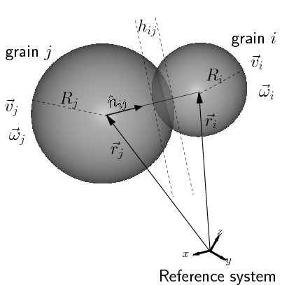
Parameter	Definition
$R_{i(j)}$	Radius of particle $i(j)$
$z_{i(j)}$	Position of the contact point $i(j)$
$R_{i(j)}^{\prime}=R_{i(j)}-z_{i(j)}$	Corrected Radius of particle $i(j)$
$V_{i}=\dfrac{E_{i}}{1-\nu^{2}}$	Stiffness of grain $i$
$E_{i}$	Young modulus of grain $i$
$\nu_{i}$	Poisson modulus of grain $i$
$\hat{n}_{ij}$	Normal unitary vector
$\hat{t}_{ij}$	Normal tangential vector
$\vec{B}^{n}$	Normal component of vector $\vec{B}$
$\vec{B}^{t}$	Tangential component of vector $\vec{B}$
$m_{ij}$	Reduced mass
$\theta_{r}$	Rolling angle

Table 1: Parameter definitions of the microscopic model

The total force in normal direction is given by

$$\vec{F}_{ij}^{n}=\frac{4}{3}\sqrt{\frac{R_{i}R_{j}}{R_{i}+R_{j}}}\frac{V_{i}V_{j}}{V_{i}+V_{j}} h_{ij}^{3/2}\hat{n}_{ij}$$

$$-\frac{m_{i}m_{j}}{m_{i}+m_{j}}\gamma_{n}\sqrt{h_{ij}}\vec{v}_{ij}^{n},$$ (1)

where the first term is the Hertz elastic force and the second one is a normal damping force that reproduces the experimental effect of the restitution coefficient [11, 12]. The variable $h_{ij}=R_{i}+R_{j}-|\vec{r}_{i}-\vec{r}_{j}|$ is the inter-penetration distance between particles. The normal unitary vector is computed as  $\hat{n}_{ij}=(\vec{r}_{i}-\vec{r}_{j})/|\vec{r}_{i}-\vec{r}_{j}|$. In all cases but static friction, the tangential unitary vector is computed as $\hat{t}_{ij}=\vec{v}_{ij}^{t}/|\vec{v}_{ij}^{t}|$, where $\vec{v}_{ij}^{t}$ is the tangential component of the relative velocity. In addition, in the normal direction we have a torque that slows down the relative angular rotations on the normal direction. As an alternative to the traditional Cundall-Strack approach [13, 14], we derived a new expression for this torque [15]. It reads

$$\vec{\tau}_{ij}=-4\pi\gamma_{nt}m_{ij}R_{ij}h_{ij}\vec{\omega}_{ij}^{n}.$$ (2)

This expression can be deduced in the following way: when two grains are touching each other and have a non-null relative angular velocity on the normal direction, the contact surface of one grain rotates relative to the other one. For each area element on the contact surface we assign a kinetic friction force that opposes to the relative motion. The net sum of this forces is zero, since they cancels in pairs, but the torque does not cancel. By summing up all torque contributions on the contact surface, we obtain (2). This expression depends on the reduced radius and the penetration depth as a consequence of the geometry of the contact surface without additional assumptions.

On the tangential direction, the forces acting between grains depend on the relative position and motion. Furthermore, in order to compute the torque we need to define the location of the contact point c, i.e. the point where the forces are applied. It is usual to define c to be in the middle of the contact surface, despite the polydispersity of the sample, but one can show by simple geometrical arguments that this point c is located at [15]

$$z_{i(j)}=h_{ij}\frac{R_{j(i)}}{R_{i}+R_{j}}.$$ (3)

The value $z_{i(j)}$$=$$h_{ij}/2$ requires $R_{i}$$=$$R_{j}$.

In order to compute the sliding friction force and torque, we check out the value of the tangential relative sliding velocity at the contact point,

$$\vec{v}_{pij}=\vec{v}_{pi}-\vec{v}_{pj}=\vec{v}_{i}-\vec{v}_{j}-(R_{i}^{\prime}\vec{\omega}_{i}+R_{j}^{\prime}\vec{\omega}_{j})\times\hat{n}_{ij}.$$ (4)

If this velocity is different from zero, the particles are sliding and we apply the following force and torque:

$$\vec{F}^{t}_{ij}=-\mu_{k}|\vec{F}^{n}|\hat{t}_{ij},$$ (5)

$$\vec{\tau}_{ij}=-R_{i}^{\prime}\hat{n}_{ij}\times\vec{F}^{t}_{ij}.$$ (6)

If the sliding velocity is almost null (in fact, less than a small predefined velocity) we compute the objective rolling velocity [14] as

$$\vec{v}_{pij}=\vec{v_{p}}_{ji}=\vec{v}_{pij}^{t}=R_{ij}^{\prime}(\vec{\omega}_{i}-\vec{\omega}_{j})\times\hat{n}_{ij},$$ (7)

where $R_{ij}^{\prime}$ is the reduced effective radius. If this velocity is non-null, the particles are rolling. By extending the rolling model to three dimensions and applying on two soft spherical bodies we obtain the following expression for the rolling friction force and torque [15],

$$\vec{F}^{t}_{ij} =-\frac{|\vec{F}^{n}|\tan\theta_{r}}{1+I/m_{i}{R_{i}^{\prime}}^{2}}\ \hat{t}_{ij},$$ (8)

$$\vec{\tau}_{ij} =\frac{R_{i}^{\prime}|\vec{F}^{n}|\tan\theta_{r}}{1+m_{i}{R_{i}^{\prime}}^{2}/I}\ \hat{t}_{ij}\times\hat{n}_{ij},$$ (9)

where the rolling constraint is clear. Finally, if the particles are not sliding and not rolling over each other, they are in relative rest. But, if there is a tangential relative force, the particles could not stay in rest unless a tangential static friction force is present. In this case the tangential unitary vector $\hat{t}_{ij}$ is computed from the tangential force as $\hat{t}_{ij}=\vec{F}^{t}/|\vec{F}^{t}|$. For the static friction force we apply a simplified model [16],

$$\vec{F}_{ij}^{t}=-\vec{F}^{t},\text{if $|\vec{F}^{t}|<\mu_{s}|\vec{F}_{ij}^{n}|$}.$$ (10)

With the model presented so far we were able to reproduce complex behaviors as sliding or rolling and dissipation on both normal and tangential directions. We tested each force implementation by making particular simulations for each of the following cases: sliding, rolling, only static friction and normal dissipation. For each case the model worked properly and also for the case with all the interactions turned on.

3 Integration methods

The simulation method we used is Molecular Dynamics (MD), also known as Discrete Element Method (DEM). In MD, the time evolution is traced on discrete time steps of size $\delta t$. The size of $\delta t$ depends on the mechanical and geometrical properties of the system and is typically of the order $O(\delta t)\simeq 10^{-5}-10^{-7}$ s. The MD computes the next positions and velocities (or the next angular orientation and angular velocities) by solving the second Newton law for each particle in terms of the current positions, velocities and forces (or the current orientation, angular velocities and torques). This needs not only a model for the forces and torques, as given in Section 2, but also an integration algorithm.

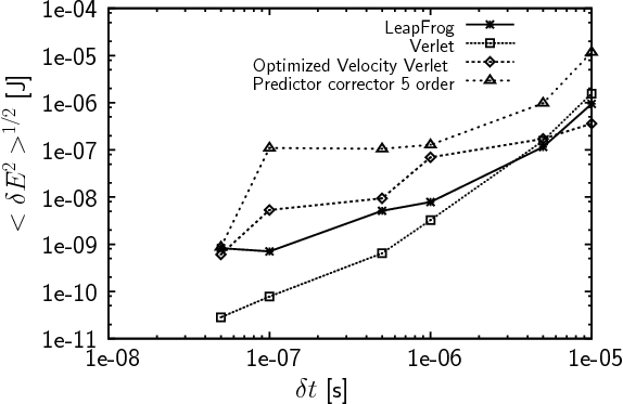
There exists many different integration algorithms for the translation and rotation variables. The choice of one algorithm over another depends on the forces, the system size and the total simulation time. In order to choose one integration algorithm for the translational variables we investigated the conservation of energy in a system of 50 particles colliding with the Hertz force in a rectangular box. The implemented translational integration algorithms were: Verlet [17, 18], Leap-Frog [17, 18], optimized Velocity Verlet  [19, 20] and a fifth-order predictor-corrector method [17]. The optimized velocity Verlet method is written as

$$\vec{R}_{1}=\vec{R}(t)+\vec{V}(t)\xi\delta t,$$ (11)

$$\vec{V}_{1}=\vec{V}(t)+\frac{1}{m}\vec{F}[\vec{R}_{1}]\delta t/2,$$ (12)

$$\vec{R}_{2}=\vec{R}_{1}+\vec{V}_{1}(1-2\xi)\delta t,$$ (13)

$$\vec{V}(t+\delta t)=\vec{V}_{1}+\frac{1}{m}\vec{F}[\vec{R}_{2}]\delta t/2,$$ (14)

$$\vec{R}(t+\delta t)=\vec{R}_{2}+\vec{V}(t+\delta t)\xi\delta t,$$ (15)

where $\vec{R},\vec{V}$ and $\vec{F}$ represents the particle position, velocity and force, respectively. The parameter $\xi\simeq 0.193183325037836$  minimizes the total truncation error of the algorithm [19]. For each time step, two computations of the forces are needed, but even doubling the time step makes the errors three times smaller than in the original Velocity Verlet algorithm ($\xi=0)$. Figure 2 shows the variation of the total mechanic energy $\langle\delta E^{2}\rangle^{1/2}=(\langle E^{2}\rangle-\langle E\rangle^{2})^{1/2}$, averaged over the total simulation time, as a function of the time step $\delta t$. It is clear that for large $\delta t$ the best algorithm is the optimized velocity Verlet method. This is the algorithm we chose for the translational motion.

Figure 2: Variation of the total mechanic energy as a function of the time step $\delta t$ for different translation integration algorithms.

The simulation of spatial rotations is more complicated. It is well known that the Euler angles can keep the information of a rigid body on space, but there are some numerical instabilities on using them [17, 18]. For this reason, the Euler angles are replaced by unitary quaternions, denoted here by $\mathbf{q}$, and the numerical problems are solved. The main disadvantages on using quaternions are the absence of high order integration algorithms and the need to normalize the quaternion at each time step. These problems are solved in a new formulation proposed by Omelyan [21] of the Leap-Frog method for quaternions that preserves the quaternion unit norm, despite the size of the discrete time step.

In the original paper, the Omelyan algorithm is formulated in the $y$ convention of the Euler angles. We rewrote it on the $x$ convention,

$$\begin{pmatrix}\dot{}q_{0}\\ \dot{}q_{1}\\ \dot{}q_{2}\\ \dot{}q_{3}\\ \end{pmatrix}=\frac{1}{2}\begin{pmatrix}0&-\omega_{x}^{b}&-\omega_{y}^{b}&-\omega_{z}^{b}\\ \omega_{x}^{b}&0&\omega_{z}^{b}&-\omega_{y}^{b}\\ \omega_{y}^{b}&-\omega_{z}^{b}&0&\omega_{x}^{b}\\ \omega_{z}^{b}&\omega_{y}^{b}&-\omega_{x}^{b}&0\\ \end{pmatrix}\begin{pmatrix}q_{0}\\ q_{1}\\ q_{2}\\ q_{3}\\ \end{pmatrix}\equiv Q(\vec{\omega})\mathbf{q},$$ (16)

while the new angular velocities and quaternions are computed as

$$\vec{\omega}^{b}\left(t+\frac{\delta t}{2}\right)=\vec{\omega}^{b}\left(t-\frac{\delta t}{2}\right)+\frac{\delta t}{I}\vec{\tau}^{b}(t)+O(\delta t^{3}),$$ (17)

$$\mathbf{q}(t+\delta t)=\frac{I\left(1-\frac{\delta t^{2}}{16}\omega^{2}\right)+\delta tQ(\vec{\omega})}{1+\frac{\delta t^{2}}{16}\omega^{2}}\mathbf{q}(t)+O(\delta t^{3}),$$ (18)

where the superscript ^b represents the body fixed reference axes, $I$ is the identity matrix on $R^{4}$, $Q(\vec{\omega})$ is the matrix defined on (16) and the angular velocity $\vec{\omega}$ is computed in $t+\delta t/2$.

4 Simulation of the oedometric test

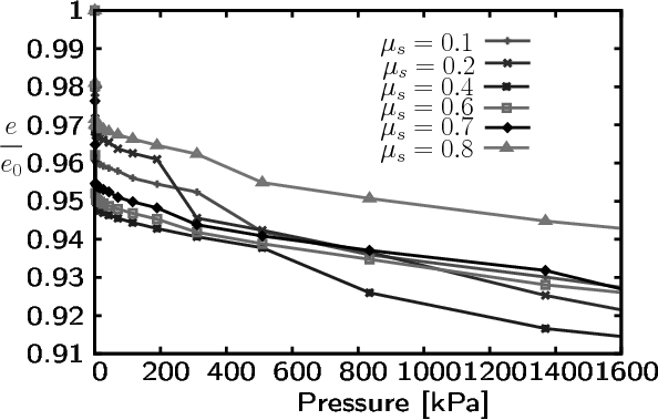
Several element tests are performed on a soil in order to measure its macroscopic parameters. An oedometric test [7] consists on filling a metallic cylinder with a sample of the soil and measuring the initial void ratio $e_{0}$, that is the ratio between the volume occupied by voids over the total volume of the sample. All cylinder walls but the top one are fixed. Then, an initial vertical pressure $p_{0}$ is applied on the top wall and, after some time (typically 10 minutes), the sample relaxes to a new void ratio. Then, the pressure is doubled, the sample relaxes and a new void ratio is measured. The procedure repeats until reaching some maximal pressure before the particles crush.

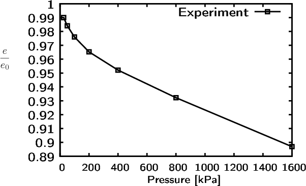
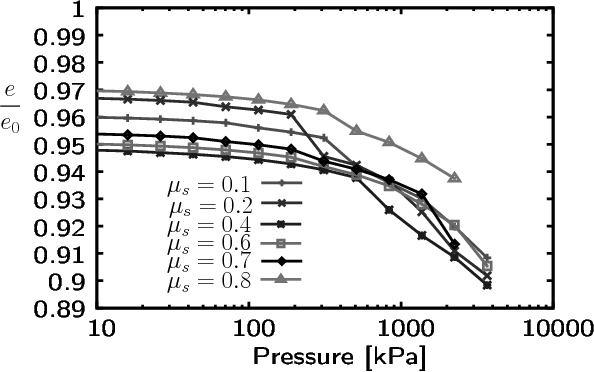
The curve so obtained (figure 3) can be fit by the Bauer empirical equation [22]

$$\frac{e}{e_{0}}=\exp\left[-\left(\frac{p}{h_{s}}\right)^{\eta}\right]\quad$$ (19)

by using, for instance, the Levenberg-Marquardt algorithm [23]. This gives the two hypoplastic parameters $h_{s}$ and $\eta$. Figure 3 shows the oedometric curve for a Guamo sand with grains between 0.85mm and 1.15mm diameter; we obtained $h_{s}[\text{MPa}]=19.1(1.1)$ and $\eta=0.57(1)$.

pb

Figure 3: Experimental oedometric test results on a dry Guamo sand in (top) linear and (bottom) log-scale on the applied vertical stress.

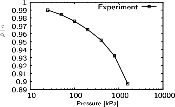
The same experimental procedure has been implemented in the simulations. For each set of microscopic parameters, the grains are randomly distributed inside the cylindrical container; they fall down by gravity and collide each other and with the walls until rest. Then, the top wall falls down with the initial pressure $p_{0}$ and the oedometric test starts, following the same procedure than in the experimental test. We try the simulation to be as similar to the experiment as possible: The dimensions of the container, the polydispersity of the sample and others parameters have almost the same experimental values. The only difference is in the number of grains: around 5000 for the experiment and 280 for the simulation (because of hardware limitations). At a first glance it appears as a very drastic reduction, but the results were very closed to the experimental data, and it gives us some confidence on the procedure. Moreover, current simulations with more than 1000 particles shows similar behaviour to the present ones. The typical computational time for the simulation of a complete oedometric test was about 52 hours on a Pentium IV 3.0 GH machine with 4GB of RAM. The compiler used was gnu/g++. That was done for $\delta t\simeq 10^{-7}$ seconds.

Figure 4: Void ratio versus vertical stress for various values of the microscopic static friction coefficient $\mu_{s}$.

$\boldsymbol{V\text{[GPa]}}$	$\boldsymbol{\eta}$	$\boldsymbol{h_{s}\text{[MPa]}}$
0.0112	11(3) $\times 10^{-1}$	1(2) $\times 10^{-1}$
0.1125	10(3) $\times 10^{-1}$	6(6) $\times 10^{-1}$
1.1250	51(3) $\times 10^{-2}$	34(5)
18.000	24(2) $\times 10^{-2}$	5(2) $\times 10^{4}$

$\boldsymbol{\mu_{k}}$	$\boldsymbol{\eta}$	$\boldsymbol{h_{s}\text{[MPa]}}$
0.1	428(7) $\times 10^{-3}$	176(7) $\times 10^{1}$
0.2	302(3) $\times 10^{-3}$	159(6) $\times 10^{2}$
0.4	26(2) $\times 10^{-2}$	4(1) $\times 10^{4}$
0.6	40(7) $\times 10^{-2}$	13(7) $\times 10^{2}$

Table 2: Macroscopic parameters $h_{s}$ and $\eta$ for different values of the microscopic parameter $V$ (top) and $\mu_{k}$ (bottom).

Two typical curves for the simulation of the oedometric compression are shown in Figure 4. Similar curves are obtained for the other parameters by following the same procedure as before (see Tables 2 and 3 for details).

$\boldsymbol{\gamma_{n}[\text{s}^{-1}\text{m}^{-1/2}]}$	$\boldsymbol{\eta}$	$\boldsymbol{h_{s}\text{[MPa]}}$
5.0e1	287(1) $\times 10^{-3}$	250(4) $\times 10^{2}$
5.0e2	29(4) $\times 10^{-2}$	16(8) $\times 10^{3}$
5.0e3	32(2) $\times 10^{-2}$	8(1) $\times 10^{3}$
5.0e4	27(4) $\times 10^{-2}$	2(1) $\times 10^{4}$
5.0e6	26(3) $\times 10^{-2}$	4(2) $\times 10^{4}$
5.0e7	20(4) $\times 10^{-2}$	7(6) $\times 10^{4}$

$\boldsymbol{\mu_{s}}$	$\boldsymbol{\eta}$	$\boldsymbol{h_{s}\text{[MPa]}}$
0.1	26(2) $\times 10^{-2}$	32(7) $\times 10^{3}$
0.2	30(2) $\times 10^{-2}$	7(2)$\times 10^{3}$
0.4	24(1) $\times 10^{-2}$	4(1) $\times 10^{4}$
0.6	20(2) $\times 10^{-2}$	5(3)$\times 10^{5}$
0.7	19(3) $\times 10^{-2}$	10(8) $\times 10^{5}$
0.8	23(1) $\times 10^{-2}$	5(2) $\times 10^{5}$

Table 3: Macroscopic parameters $h_{s}$ and $\eta$ for different values of the microscopic parameter $\gamma_{n}$ (top) and $\mu_{s}$ (bottom).

Figure 5: $h_{s}$ as a function of $\eta$ for different values of the microscopic parameters

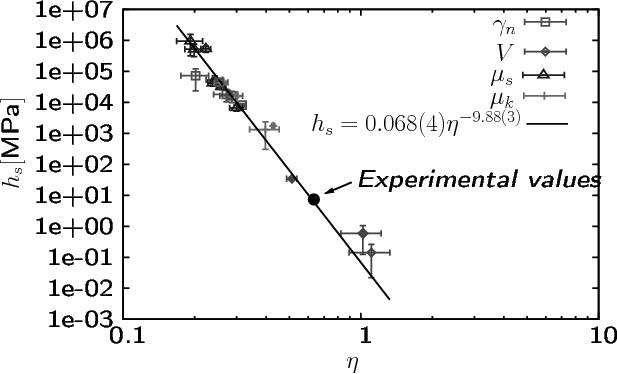
We noted that, in all cases, the two hypoplastic parameters behave in a non-independent way. When one parameter increases, the other one decreases. This suggest a hidden relationship between them. In order to investigate this relation, we plot $h_{s}$ as a function of $\eta$ for all sets of microscopic parameters, as shown in figure 5. It reveals and unsuspected power law relationship between the two hypoplastic parameters: $h_{s}$$=$$0.068(4)\eta^{-9.88(3)}$. Moreover, the experimental values lay on the line. This kind of relation could suggest a possible reduction in the number of macroscopic parameters of the hypoplastic theory, but the experimental values for different sands with different granulometries do not lay on a single power law. Let us point out that we have varied all microscopic parameters ($V$, $\gamma_{n}$, $\mu_{k}$ and $\mu_{s}$), but the granulometry. It is well known [24] that $\eta$ strongly depends on the granulometry, but once this variable is fixed, a power law could appear. This result should be validated by future experiments and simulations.

5 Conclusions

Hereby we have simulated the oedometric compression of a bad-graded Guamo sand in order to estimate the hypoplastic parameters $h_{s}$ and $\eta$, and we have compared with experimental results. In particular, we have investigated the changes on these two macroscopic parameters by varying four microscopic parameters: the stiffness $V$, the normal damping constant $\gamma_{n}$, the static friction coefficient $\mu_{s}$ and dynamic friction coefficient $\mu_{k}$. By doing so, we found an unexpected power-law relationship between $h_{s}$ and $\eta$: for our case, $h_{s}\propto\eta^{-9.88(3)}$. Moreover, the experimental values for the Guamo sand with the same granulometry (random-distributed diameters between 0.85 and 1.15mm) lies on the same curve. This suggests us that these two parameters may be replaced by other two, more related with the microscopic world: one reflecting the granulometry and another one reflecting the strength of the microscopic interactions. This power law, of course, must be confirmed by a broader set of experiments, but the possibility is very promising. The experimental confirmation of these kind of relationships and the possible definition of these two new parameters are subjects of present research.

The simulation performed is 3D and the software developed by us includes some of the state-of-the-art algorithms for spatial translation and rotations. Moreover, the microscopic force model includes rolling among the more traditional elastic and damping normal interactions and sliding and static frictional forces. The rolling process allows global dissipation and long-range reorientations without requiring a big spatial reconfiguration of the sample, that is without changing the macroscopic void ratio, and its global effect on the macroscopic parameters is very interesting to explore. For example, it would be possible to perform simulations with and without the rolling force in order to get insight into its actual role on the soil properties. This will be a topic of future work.

Micro-mechanical simulations are powerful tools for the investigation on the microscopic origin of macroscopic behavior of soils. Furthermore, these computer experiments have shown to be able to approximate the experimental parameters for the soil. We hope this work will raise new questions regarding the microscopic origin of the constitutive parameters and gives starting points for a redefinition of the macroscopic parameters, more related with the microscopic world.

References

- [1] Duran, J., Sands, Powders, and Grains: An Introduction to the Physics of Granular Materials (Partially Ordered Systems), Springer, 1 edition, 1999, P.-G.de Gennes (Foreword).
- [2] de Gennes, P. G., Reviews of Modern Physics 71 (1999) 374, Centenary 1999.
- [3] Garcia-Rojo, R., Herrmann, H. J., and S., M., editors, Powders and grains: Proceedings of the 5th International Conference on Micromechanics of Granular Media, Stuttgart, Germany, Association pour L’Etude de la Microm canique des Mileaux Granulaires, 2005, Section on the micro-macro connection.
- [4] Kolymbas, D., Mech. Res. Comm 4 (1977) 367.
- [5] Tejchman, J. and Wu, W., International Journal of Non-linear Mechanics 42 (2007) 882.
- [6] Evesque, P., Poudres & Grains (1996) 6, Also cond-mat/0506344, 2005 - arxiv.org.
- [7] Evesque, P., Poudres & Grains (1999) 1, Also cond-mat/0506335, 2005 - arxiv.org.
- [8] Alonso-Marroquin, F. and Herrmann, H. J., Physical Review Letters 92 (2004) 054301.
- [9] Rapaport, D. C., The Art of Molecular Dynamics Simulation, Cambridge University Press, second edition edition, 2004, Chapter 16 Granular Dynamics.
- [10] Patiño, J. C. and Lizcano, A., (2004), Working paper.
- [11] Ramírez, R., Pöschel, T., Brilliantov, N. V., and Schwager, T., Phys. Rev. E 60 (1999) 4465.
- [12] Kruggel-Emden, H., Simseck, E., Rickelt, S., Wirtz, S., and Scherer, V., Powder Technology 171 (2007) 157.
- [13] Herrmann, H. J. and Luding, S., Continuum Mech. Thermodyn. 10 (1998) 198.
- [14] Luding, S., Granular Matter 10 (2008) 235.
- [15] Oquendo, W. F., Simulación de la compresión edométrica de un material granular y determinación de la relación de vacíos (simulation of the oedometric test of a granular material and determination of the void relation), Master’s thesis, Universidad Nacional de Colombia (national University of Colombia), 2007.
- [16] Olsson, H., Åström, K. J., Canudas de Wit, C., Gäfvert, M., and Lichinsky, P., European Journal Of Control 4 (1998) 176.
- [17] Rapaport, D. C., The Art of Molecular Dynamics Simulation, Cambridge University Press, second edition edition, 2004, Molecular Dynamics.
- [18] Allen, M. P. and Tildesley, D. J., Computer Simulation of Liquids, Oxford University Press, 1987, Molecular Dynamics.
- [19] Omelyan, I. P., Mryglod, I. M., and Folk, R., (2003), arXiv:cond-mat/0110438 v1.
- [20] Omelyan, I. P., Mryglod, I. M., and Folk, R., Phys. Rev. E 65 (2002) 056706.
- [21] Omelyan, I. P., Phys. Rev. E 58 (1998) 1169.
- [22] Bauer, E., Mechanics of Materials 31 (1999) 597.
- [23] Press, W. H., Saul, A. T., Vetterling, W. T., and Flannery, B. P., Numerical Recipes in C: The Art of Scientific Computing, Cambrige University Press, 1992.
- [24] Herle, I. and Gudehus, G., Mechanics of Cohesive-Frictional Materials 4 (1999) 461.