SELF-CONSISTENT RPA BASED ON A MANY-BODY VACUUM

Mohsen Jemaï1 and Peter Schuck2,3 email: jemai@ipno.in2p3.fremail: schuck@ipno.in2p3.fr 1Département de Physique, Faculté des Sciences de Tunis, Université Tunis El Manar, 2092 El Manar, Tunis, Tunisie
2Institut de Physique Nucléaire d’Orsay, Université Paris-Sud, CNRS–IN2P3 15, Rue Georges Clemenceau, 91406 Orsay Cedex, France
3Laboratoire de Physique et Modélisation des Milieux Condensés (LPMMC) (UMR 5493), Maison Jean Perrin, 25 avenue des Martyrs BP 166, 38042 Grenoble cedex 9, France
Abstract

Self-Consistent RPA is extended in a way so that it is compatable with a variational ansatz for the ground state wave function as a fermionic many-body vacuum. Employing the usual equation of motion technique, we arrive at extended RPA equations of the Self Consistent RPA structure. In principle the Pauli principle is, therefore, fully respected. However, the correlation functions entering the RPA matrix can only be obtained from a systematic expansion in powers of some combinations of RPA amplitudes. We demonstrate for a model case that this expansion may converge rapidly.

pacs:
71.10.-w, 75.10.Jm, 72.15.Nj

I Introduction

The many body problem still being to a great deal an unsolved problem, new vistas are welcome. We here present an extension of Self-Consistent RPA art1 which is based on a fermionic many body wave function being the vacuum to an extended RPA destruction operator. Let us expose the main ideas before entering the details of the theory and making an application to a model case. In this work we will consider interacting fermions, however, the extension to the bosonic case is possible.
Many-body theories have a clear cut hirarchy: one body, two body, …, etc. One body theories are mean field theories. One can write down a variational wave function for the ground state

|Z(1)=ephzph(1)cpch|ϕketsuperscript𝑍1superscript𝑒subscript𝑝superscriptsubscript𝑧𝑝1superscriptsubscript𝑐𝑝subscript𝑐ketitalic-ϕ|Z^{(1)}\rangle=e^{\sum_{ph}z_{ph}^{(1)}c_{p}^{\dagger}c_{h}}|\phi\rangle (1)

where zph(1)superscriptsubscript𝑧𝑝1z_{ph}^{(1)} are variational parameters and |ϕ=hch|vacketitalic-ϕsubscriptproductsuperscriptsubscript𝑐ket𝑣𝑎𝑐|\phi\rangle=\prod_{h}c_{h}^{\dagger}|vac\rangle is an arbitrary Slater determinant built from an antisymmetric product of N𝑁N fermion creators in the lowest levels, the so-called hole (h) levels below the Fermi energy. One can explicitly evaluate the expectation value of, e.g. a two body Hamiltonian

E0[z(1)]=Z(1)|H|Z(1)Z(1)|Z(1)subscript𝐸0delimited-[]superscript𝑧1quantum-operator-productsuperscript𝑍1𝐻superscript𝑍1inner-productsuperscript𝑍1superscript𝑍1E_{0}[z^{(1)}]=\frac{\langle Z^{(1)}|H|Z^{(1)}\rangle}{\langle Z^{(1)}|Z^{(1)}\rangle} (2)

and minimise with respect to the parameters zph(1)superscriptsubscript𝑧𝑝1z_{ph}^{(1)}. This leads to the well known Hartree-Fock (HF) equations. That this program can be pulled through hinges to a large extent on the fact that |Z(1)ketsuperscript𝑍1|Z^{(1)}\rangle is the vacuum of quasiparticle operators apexp(Z(1))cpexp(Z(1))=cp+hzph(1)chproportional-tosubscript𝑎𝑝𝑒𝑥𝑝superscript𝑍1subscript𝑐𝑝𝑒𝑥𝑝superscript𝑍1subscript𝑐𝑝subscriptsubscriptsuperscript𝑧1𝑝subscript𝑐a_{p}\propto exp(-Z^{(1)})c_{p}exp(Z^{(1)})=c_{p}+\sum_{h}z^{(1)}_{ph}c_{h} and similiar for ahsuperscriptsubscript𝑎a_{h}^{\dagger}, with ah|Z(1)=ap|Z(1)=0superscriptsubscript𝑎ketsuperscript𝑍1subscript𝑎𝑝ketsuperscript𝑍10a_{h}^{\dagger}|Z^{(1)}\rangle=a_{p}|Z^{(1)}\rangle=0. The scheme clearly is of the Raleigh-Ritz (RR) form stating that the so obtained energy is an upper bound to the true ground state energy.
Unfortunately, on the next level, i.e. the two body correlations, there does not exist such a nice closed formalism with RR character. As a consequence several approaches to two body and higher order correlation functions have been elaborated. Some try to be RR variational, some not. For example, the so-called hypernetted chain or Jastrow approach puts a local, usually translational invariant, two body operator in the exponent, with u(𝐫𝐫)𝑢𝐫superscript𝐫u(\mathbf{r}-\mathbf{r}^{\prime}) the corresponding variational parameters. This leads to a chain of equations, the solution of which may eventually converge to the exact RR variational solution of the corresponding energy, depending on at which level the chain is broken off art2 . The Gutzwiller ansatz art3 is taylored to the electron gas on a lattice and puts another two body operator in the exponent penalising double occupancies. However, the variation usually cannot be pulled through exactly. Most of the time one is satisfied with the approximate solution given by the so-called Gutzwiller equations art4 . Coupled Cluster Theory (CCT) is an approach art5 starting also with a two body operator in the exponent (plus eventually higher order operators) but does not lead to a RR scheme, at least not in its original form. Other non RR schemes are based on the BBGKY hirarchy of time dependent density matrices (TDDM). On this subject, there have been some interesting developments, recently art6 . In the past, several authors, including ourselves, tried to improve RPA as much as possible to overcome certain deficiencies for the calculation of two body correlation functions. It is, e.g., well known that standard RPA (s-RPA) yields two body correlations functions which violate the Pauli principle due to the so-called quasi-boson approximation inherent to s-RPA (we define s-RPA as being the small amplitude limit of TDHF implying that the exchange term is included). Usually this leads to a quite strong overbinding of the ground state energy whereas excitation energies may be more correct. We here will formulate the RPA as a diagonalisation problem as is most appropriate for finite Fermi systems, since a good part of the spectrum consists of discrete levels. In this way one usually writes the RPA excitation operator as art7

Qν+=ph(XphνapahYphνahap)superscriptsubscript𝑄𝜈subscript𝑝superscriptsubscript𝑋𝑝𝜈superscriptsubscript𝑎𝑝subscript𝑎superscriptsubscript𝑌𝑝𝜈superscriptsubscript𝑎subscript𝑎𝑝Q_{\nu}^{+}=\sum\limits_{ph}(X_{ph}^{\nu}a_{p}^{\dagger}a_{h}-Y_{ph}^{\nu}a_{h}^{\dagger}a_{p}) (3)

with k=(p,h)𝑘𝑝k=(p,h) the (particle, hole) levels. The excited state is then written as

|ν=Qν+|0ket𝜈superscriptsubscript𝑄𝜈ket0|\nu\rangle=Q_{\nu}^{+}|0\rangle (4)

where |0ket0|0\rangle is the ground state so that it is the vacuum to the destructors Qνsubscript𝑄𝜈Q_{\nu}, i.e.

Qν|0=0ν.subscript𝑄𝜈ket00for-all𝜈.Q_{\nu}|0\rangle=0~{}~{}~{}~{}~{}~{}\forall~{}\nu\mbox{.} (5)

Since this scheme cannot be pulled through in general, in s-RPA the so-called quasi boson approximation is introduced replacing the fermion pair operators by ideal Bose operators art7

apahBph+superscriptsubscript𝑎𝑝subscript𝑎superscriptsubscript𝐵𝑝a_{p}^{\dagger}a_{h}\rightarrow B_{ph}^{+} (6)

with

[Bph,Bph+]=δppδhh.subscript𝐵𝑝superscriptsubscript𝐵𝑝subscript𝛿𝑝superscript𝑝subscript𝛿superscript.\left[B_{ph},B_{ph}^{+}\right]=\delta_{pp^{\prime}}\delta_{hh^{\prime}}\mbox{.} (7)

In this way, (3) boils down to a Bogoliubov transformation among ideal bosons with the usual HFB vacuum art7

|0e(1/4)zp1p2h1h2(B)Bp1h1+Bp2h2+|HF)|0\rangle\rightarrow e^{(1/4)\sum z_{p_{1}p_{2}h_{1}h_{2}}^{(B)}B_{p_{1}h_{1}}^{+}B_{p_{2}h_{2}}^{+}}|HF) (8)

with ahap|HFBph|HF)=0a_{h}^{\dagger}a_{p}|HF\rangle\rightarrow B_{ph}|HF)=0. Since a fermion Hamiltonian can be expanded via Holstein-Primakoff or Belyaev-Zelevinsky boson expansion in powers of the boson operators art7 , the RPA ends up with a standard HFB approach for interacting bosons. The scheme approaches, of course, a RR variational procedure only in as much as the boson expansion of the Hamiltonian converges.
In the past, we used the RPA operator (3) with the fermion pair operators, supposing that the killing condition Qν|0=0subscript𝑄𝜈ket00Q_{\nu}|0\rangle=0 existed. However, a corresponding vacuum can only be constructed in some very simplified model cases (see, e.g. art8 ) and, thus, in general, the hypothesis of the existence of a vacuum remained an approximation what perturbed the internal consistency of the so-called Self Consistent RPA (SCRPA) approach art1 ; art8 ; art9 . In this work we will adopt the strategy to keep in (8) instead of the boson operators the original fermion pair operators. We then will see that this ground state still is vacuum to a generalised RPA operator containing the standard operator (3) plus, in addition, specific two body operators correcting for the Pauli principle. With that RPA operator we will set up the familiar equation of motion (EOM) method art7 . The problem will be to evaluate the expectation values of the commutators, since the new RPA operator is non linear, i.e. not of the form of a canonical transformation. Therefore, an effective systematic expansion scheme will be set up for these expectation values. The procedure will be applied to the very schematic two level Lipkin model where it is shown that the expansion converges fast, even for very small particle numbers.

II General Theory

As mentioned in the introduction, we will consider the following variational ansatz for the many body ground state

|0|Z(2)=eZ(2)|HFket0ketsuperscript𝑍2superscript𝑒superscript𝑍2ket𝐻𝐹|0\rangle\equiv|Z^{(2)}\rangle=e^{Z^{(2)}}|HF\rangle (9)

with

Z(2)=14zp1p2h1h2(2)ap1ah1ap2ah2superscript𝑍214superscriptsubscript𝑧subscript𝑝1subscript𝑝2subscript1subscript22superscriptsubscript𝑎subscript𝑝1subscript𝑎subscript1superscriptsubscript𝑎subscript𝑝2subscript𝑎subscript2Z^{(2)}=\frac{1}{4}\sum z_{p_{1}p_{2}h_{1}h_{2}}^{(2)}a_{p_{1}}^{\dagger}a_{h_{1}}a_{p_{2}}^{\dagger}a_{h_{2}} (10)

where zp1p2h1h2(2)superscriptsubscript𝑧subscript𝑝1subscript𝑝2subscript1subscript22z_{p_{1}p_{2}h_{1}h_{2}}^{(2)} are the variational parameters. In general they can be complex. In principle we can add a one body operator as in (1) to the exponent and vary z(1)superscript𝑧1z^{(1)} and z(2)superscript𝑧2z^{(2)} simultaneously. In order to keep the formalism as transparent as possible, we will refrain from this complication here and suppose that we work in the standard HF basis. The first task will be to find an RPA operator Qν+superscriptsubscript𝑄𝜈Q_{\nu}^{+} which applied to |Z(2)ketsuperscript𝑍2|Z^{(2)}\rangle gives the excited states of the system: |ν=Qν+|Z(2)ket𝜈superscriptsubscript𝑄𝜈ketsuperscript𝑍2|\nu\rangle=Q_{\nu}^{+}|Z^{(2)}\rangle and whose hermitian conjugate kills the ground state acting, therefore, as a vacuum

Qν|Z(2)=0ν.subscript𝑄𝜈ketsuperscript𝑍20for-all𝜈.Q_{\nu}|Z^{(2)}\rangle=0~{}~{}~{}~{}~{}~{}\forall~{}\nu\mbox{.} (11)

We make the following ansatz for the destruction operatorart10

Qν=ph[XphνahapYphνapah]subscript𝑄𝜈subscript𝑝delimited-[]superscriptsubscript𝑋𝑝𝜈superscriptsubscript𝑎subscript𝑎𝑝superscriptsubscript𝑌𝑝𝜈superscriptsubscript𝑎𝑝subscript𝑎\displaystyle Q_{\nu}=\sum\limits_{ph}\left[X_{ph}^{\nu}a_{h}^{\dagger}a_{p}-Y_{ph}^{\nu}a_{p}^{\dagger}a_{h}\right]
+12php1p2ηp1pp2hνap2ap1apah12subscript𝑝subscript𝑝1subscript𝑝2superscriptsubscript𝜂subscript𝑝1𝑝subscript𝑝2𝜈superscriptsubscript𝑎subscript𝑝2subscript𝑎subscript𝑝1superscriptsubscript𝑎𝑝subscript𝑎\displaystyle+\frac{1}{2}\sum\limits_{php_{1}p_{2}}\eta_{p_{1}pp_{2}h}^{\nu}a_{p_{2}}^{\dagger}a_{p_{1}}a_{p}^{\dagger}a_{h}
12phh1h2ηph1hh2νah1ah2apah12subscript𝑝subscript1subscript2superscriptsubscript𝜂𝑝subscript1subscript2𝜈superscriptsubscript𝑎subscript1subscript𝑎subscript2superscriptsubscript𝑎𝑝subscript𝑎\displaystyle-\frac{1}{2}\sum\limits_{phh_{1}h_{2}}\eta_{ph_{1}hh_{2}}^{\nu}a_{h_{1}}^{\dagger}a_{h_{2}}a_{p}^{\dagger}a_{h} (12)

with

Yphν=p1h1Xp1h1νzp1ph1h(2)superscriptsubscript𝑌𝑝𝜈subscriptsubscript𝑝1subscript1superscriptsubscript𝑋subscript𝑝1subscript1𝜈superscriptsubscript𝑧subscript𝑝1𝑝subscript12Y_{ph}^{\nu}=\sum\limits_{p_{1}h_{1}}X_{p_{1}h_{1}}^{\nu}z_{p_{1}ph_{1}h}^{(2)} (13)

and

ηp1pp2hν=h1Xp1h1νzpp2hh1(2),superscriptsubscript𝜂subscript𝑝1𝑝subscript𝑝2𝜈subscriptsubscript1superscriptsubscript𝑋subscript𝑝1subscript1𝜈superscriptsubscript𝑧𝑝subscript𝑝2subscript12\eta_{p_{1}pp_{2}h}^{\nu}=\sum\limits_{h_{1}}X_{p_{1}h_{1}}^{\nu}z_{pp_{2}hh_{1}}^{(2)}, (14)
ηph1hh2ν=p1Xp1h1νzpp1hh2(2).superscriptsubscript𝜂𝑝subscript1subscript2𝜈subscriptsubscript𝑝1superscriptsubscript𝑋subscript𝑝1subscript1𝜈superscriptsubscript𝑧𝑝subscript𝑝1subscript22.\eta_{ph_{1}hh_{2}}^{\nu}=\sum\limits_{p_{1}}X_{p_{1}h_{1}}^{\nu}z_{pp_{1}hh_{2}}^{(2)}\mbox{.} (15)

We indeed verify that Qνsubscript𝑄𝜈Q_{\nu} kills the ground state (9). The amplitudes X,Y𝑋𝑌X,Y can be normalised according to 0|[Qν,Qν+]|0=1quantum-operator-product0subscript𝑄𝜈superscriptsubscript𝑄𝜈01\langle 0|[Q_{\nu},Q_{\nu}^{+}]|0\rangle=1. Evidently (12) contains the usual RPA operator (3) plus extra specific 2-body operators. These extra terms serve to fullfil the Pauli principle. They make, however, the calculus rather heavy. In the following, we shortly outline our approach and then give an application to a schematic model.
In order to determine the amplitudes X,Y𝑋𝑌X,Y, we proceed as usual and minimisethe following mean excitation energy, equivalent to the minimisation of an (symmetrised) energy weighted sum rule art9 ,

Ων=0|[Qν,[H,Qν+]]|0+0|[[Qν,H],Qν+]|020|[Qν,Qν+]|0.subscriptΩ𝜈quantum-operator-product0subscript𝑄𝜈𝐻superscriptsubscript𝑄𝜈0quantum-operator-product0subscript𝑄𝜈𝐻superscriptsubscript𝑄𝜈02quantum-operator-product0subscript𝑄𝜈superscriptsubscript𝑄𝜈0.\Omega_{\nu}=\frac{\langle 0|[Q_{\nu},[H,Q_{\nu}^{+}]]|0\rangle+\langle 0|[[Q_{\nu},H],Q_{\nu}^{+}]|0\rangle}{2\langle 0|[Q_{\nu},Q_{\nu}^{+}]|0\rangle}\mbox{.} (16)

Using in this expression the standard RPA operator Qν+=XphνapahYphνahapsuperscriptsubscript𝑄𝜈superscriptsubscript𝑋𝑝𝜈superscriptsubscript𝑎𝑝subscript𝑎superscriptsubscript𝑌𝑝𝜈superscriptsubscript𝑎subscript𝑎𝑝Q_{\nu}^{+}=\sum X_{ph}^{\nu}a_{p}^{\dagger}a_{h}-Y_{ph}^{\nu}a_{h}^{\dagger}a_{p}, we obtain from the minimisation of (16) with respect to the amplitudes X𝑋X and Y𝑌Y the usual structure of the (Self Consistent) RPA equations. However, with (8) the RPA equations become more complicated. Among other things, this stems from the fact that the norm matrix is now non diagonal, i.e. the structure of the equations is as follows

(R11R12R21R22)(XY)=Ων(N11N12N21N22)(XY)subscript𝑅11subscript𝑅12subscript𝑅21subscript𝑅22𝑋𝑌subscriptΩ𝜈subscript𝑁11subscript𝑁12subscript𝑁21subscript𝑁22𝑋𝑌\left(\begin{array}[]{cc}R_{11}&R_{12}\\ R_{21}&R_{22}\end{array}\right)\left(\begin{array}[]{c}X\\ Y\end{array}\right)=\Omega_{\nu}\left(\begin{array}[]{cc}N_{11}&N_{12}\\ N_{21}&N_{22}\end{array}\right)\left(\begin{array}[]{c}X\\ Y\end{array}\right) (17)

with obvious definitions of the matrices R𝑅R and N𝑁N. They are hermitian matrices by construction, i.e. R=R+𝑅superscript𝑅R=R^{+} and N=N+𝑁superscript𝑁N=N^{+}. In order to arrive at the usual structure, we write N=N~1/2N0N~1/2𝑁superscript~𝑁12subscript𝑁0superscript~𝑁12N=\tilde{N}^{1/2}N_{0}\tilde{N}^{1/2} with

N0=(1001)subscript𝑁01001N_{0}=\left(\begin{array}[]{cc}1&0\\ 0&-1\end{array}\right) (18)

and obtain in short hand notation

R~χ~=ΩνN0χ~~𝑅~𝜒subscriptΩ𝜈subscript𝑁0~𝜒\tilde{R}\tilde{\chi}=\Omega_{\nu}N_{0}\tilde{\chi} (19)

with R~=N~1/2RN~1/2~𝑅superscript~𝑁12𝑅superscript~𝑁12\tilde{R}=\tilde{N}^{-1/2}R\tilde{N}^{-1/2} and χ~=N~1/2χ~𝜒superscript~𝑁12𝜒\tilde{\chi}=\tilde{N}^{1/2}\chi. This equation now has globally the same mathematical structure as standard RPA or SCRPA (details are different, of course). In particular, we have for the normalisation X~2Y~2=1superscript~𝑋2superscript~𝑌21\tilde{X}^{2}-\tilde{Y}^{2}=1. Of course, the task is not finished. The difficulty resides in how to express the correlation functions in R~~𝑅\tilde{R} and N~~𝑁\tilde{N} by the amplitudes X~,Y~~𝑋~𝑌\tilde{X},\tilde{Y}, since the form (12) of the RPA operator, as already mentioned, does not constitute a canonical transformation among operators and can, therefore, not be inverted in a straightforward manner. We will set up an expansion scheme which can be paraphrased as follows: Suppose we did not know how to invert the Bogoliubov transformation from ordinary to quasiparticles in standard BCS theory. How to calculate expectation values in the BCS state nontheless? Among other ways, this can go as follows. As is well known, the BCS state can be written as a coherent state: |BCS=exp[zkckck]|vacket𝐵𝐶𝑆𝑒𝑥𝑝delimited-[]subscript𝑧𝑘superscriptsubscript𝑐𝑘superscriptsubscript𝑐𝑘ket𝑣𝑎𝑐|BCS\rangle=exp[\sum z_{k}c_{k}^{\dagger}c_{-k}^{\dagger}]|vac\rangle. We want to calculate, e.g. the pairing tensor κk=BCS|ckck|BCS/BCS|BCSsubscript𝜅𝑘quantum-operator-product𝐵𝐶𝑆subscript𝑐𝑘subscript𝑐𝑘𝐵𝐶𝑆inner-product𝐵𝐶𝑆𝐵𝐶𝑆\kappa_{k}=\langle BCS|c_{-k}c_{k}|BCS\rangle/\langle BCS|BCS\rangle. We have ck|BCS=zkck|BCSsubscript𝑐𝑘ket𝐵𝐶𝑆subscript𝑧𝑘superscriptsubscript𝑐𝑘ket𝐵𝐶𝑆c_{k}|BCS\rangle=z_{k}c_{-k}^{\dagger}|BCS\rangle. Multiplying this relation with cksubscript𝑐𝑘c_{-k} and repeating the operation leads to the well known BCS expression κk=ukvksubscript𝜅𝑘subscript𝑢𝑘subscript𝑣𝑘\kappa_{k}=u_{k}v_{k} where we supposed for simplicity zksubscript𝑧𝑘z_{k} to be real, i.e. ckck=ckckdelimited-⟨⟩subscript𝑐𝑘subscript𝑐𝑘delimited-⟨⟩subscriptsuperscript𝑐𝑘subscriptsuperscript𝑐𝑘\langle c_{-k}c_{k}\rangle=\langle c^{\dagger}_{k}c^{\dagger}_{-k}\rangle, and used zk=vk/uksubscript𝑧𝑘subscript𝑣𝑘subscript𝑢𝑘z_{k}=v_{k}/u_{k} with uk2+vk2=1superscriptsubscript𝑢𝑘2superscriptsubscript𝑣𝑘21u_{k}^{2}+v_{k}^{2}=1. Using an analogous method to calculate the correlation functions in the RPA matrix leads to a series which, unfortunately, does not break off after a low number of terms unless one deals with very few particle states. As the example with the BCS state shows however, the series contains nontrivial terms and may, thus, converge rapidly. If convergence is achieved, Pauli principle is respected fully, since the theory is based on a wave function. Of course, the final success will depend on that supposed rate of convergence. This ends the rough outline of the theory. Let us now make an application to the Lipkin model which often has served in the past as a testing ground for many body theories. We will see how in that model the series expansion works and that in this case the convergence of the series is, indeed, fast and performant.

III Aplication to a schematic model

In this section we want to apply our theory to the schematic Lipkin model art11 which is an exactly solvable two level model with separable monopole-monopole interaction. The Hamiltonian is given by art7 (without loss of generality we put the intershell spacing ε=1𝜀1\varepsilon=1)

H=J^0V2(J^+2+J^2)𝐻subscript^𝐽0𝑉2superscriptsubscript^𝐽2superscriptsubscript^𝐽2H=\hat{J}_{0}-\frac{V}{2}\left(\hat{J}_{+}^{2}+\hat{J}_{-}^{2}\right) (20)

with V𝑉V the coupling constant and

J^0subscript^𝐽0\displaystyle\hat{J}_{0} =\displaystyle= 12m=1Ω(c1mc1mc0mc0m),12superscriptsubscript𝑚1Ωsuperscriptsubscript𝑐1𝑚subscript𝑐1𝑚superscriptsubscript𝑐0𝑚subscript𝑐0𝑚\displaystyle\frac{1}{2}\sum_{m=1}^{\Omega}\left(c_{1m}^{\dagger}c_{1m}-c_{0m}^{\dagger}c_{0m}\right)\,,
J^+subscript^𝐽\displaystyle\hat{J}_{+} =\displaystyle= m=1Ωc1mc0m,J^=(J^+)superscriptsubscript𝑚1Ωsuperscriptsubscript𝑐1𝑚subscript𝑐0𝑚subscript^𝐽superscriptsubscript^𝐽\displaystyle\sum_{m=1}^{\Omega}\;c_{1m}^{\dagger}c_{0m}\,,~{}~{}~{}~{}~{}~{}~{}~{}~{}\hat{J}_{-}=(\hat{J}_{+})^{\dagger} (21)

where ΩΩ\Omega is the degeneracy of one shell. We take Ω=NΩ𝑁\Omega=N with N𝑁N the particle number, i.e. the lower shell is filled for V=0𝑉0V=0. The SU2 commutation relations are

[J^+,J^]=2J^0,[J^0,J^±]=±J^±.formulae-sequencesubscript^𝐽subscript^𝐽2subscript^𝐽0subscript^𝐽0subscript^𝐽plus-or-minusplus-or-minussubscript^𝐽plus-or-minus.\left[\hat{J}_{+},\hat{J}_{-}\right]=2\,\hat{J}_{0}\;,~{}~{}~{}~{}~{}~{}~{}~{}~{}\left[\hat{J}_{0},\hat{J}_{\pm}\right]=\pm\,\hat{J}_{\pm}\mbox{.} (22)

The variational ground state corresponding to (9) is given by

|Z=eZ^|HFket𝑍superscript𝑒^𝑍ket𝐻𝐹|Z\rangle=e^{\hat{Z}}|HF\rangle (23)

with

Z^=zJ^+J^+.^𝑍𝑧subscript^𝐽subscript^𝐽.\hat{Z}=z\hat{J}_{+}\hat{J}_{+}\mbox{.} (24)

We verify that this correlated state is vacuum to the following destruction operator art10

Q=XJ^YJ¯+𝑄𝑋subscript^𝐽𝑌subscript¯𝐽Q=X\hat{J}_{-}-Y\bar{J}_{+} (25)

with z=Y/(NX)𝑧𝑌𝑁𝑋z=Y/\left(NX\right) and

J¯+=(1ηJ^0)J^+,η=2N.formulae-sequencesubscript¯𝐽1𝜂subscript^𝐽0subscript^𝐽𝜂2𝑁.\bar{J}_{+}=\left(1-\eta\hat{J}_{0}\right)\hat{J}_{+},~{}~{}~{}~{}~{}~{}\eta=\frac{2}{N}\mbox{.} (26)

We note that the non-standard correction term is of order 1/N1𝑁1/N. In this model the matrix elements of eq.(17) are given by

R11subscript𝑅11\displaystyle R_{11} =\displaystyle= 12([J^,[H,J^+]]+[[J^,H],J^+])12delimited-⟨⟩subscript^𝐽𝐻subscript^𝐽delimited-⟨⟩subscript^𝐽𝐻subscript^𝐽\displaystyle\frac{1}{2}\left(\langle\left[\hat{J}_{-},\left[H,\hat{J}_{+}\right]\right]\rangle+\langle\left[\left[\hat{J}_{-},H\right],\hat{J}_{+}\right]\rangle\right)
R12subscript𝑅12\displaystyle R_{12} =\displaystyle= 12([J^,[H,J¯]]+[[J^,H],J¯])12delimited-⟨⟩subscript^𝐽𝐻subscript¯𝐽delimited-⟨⟩subscript^𝐽𝐻subscript¯𝐽\displaystyle-\frac{1}{2}\left(\langle\left[\hat{J}_{-},\left[H,\overline{J}_{-}\right]\right]\rangle+\langle\left[\left[\hat{J}_{-},H\right],\overline{J}_{-}\right]\rangle\right)
R21subscript𝑅21\displaystyle R_{21} =\displaystyle= 12([J¯+,[H,J^+]]+[[J¯+,H],J^+])12delimited-⟨⟩subscript¯𝐽𝐻subscript^𝐽delimited-⟨⟩subscript¯𝐽𝐻subscript^𝐽\displaystyle-\frac{1}{2}\left(\langle\left[\overline{J}_{+},\left[H,\hat{J}_{+}\right]\right]\rangle+\langle\left[\left[\overline{J}_{+},H\right],\hat{J}_{+}\right]\rangle\right)
R22subscript𝑅22\displaystyle R_{22} =\displaystyle= 12([J¯+,[H,J¯]]+[[J¯+,H],J¯])12delimited-⟨⟩subscript¯𝐽𝐻subscript¯𝐽delimited-⟨⟩subscript¯𝐽𝐻subscript¯𝐽\displaystyle\frac{1}{2}\left(\langle\left[\overline{J}_{+},\left[H,\overline{J}_{-}\right]\right]\rangle+\langle\left[\left[\overline{J}_{+},H\right],\overline{J}_{-}\right]\rangle\right) (27)

and the elements of the norm matrix,

N11subscript𝑁11\displaystyle N_{11} =\displaystyle= [J^,J^+]=2J^0delimited-⟨⟩subscript^𝐽subscript^𝐽2delimited-⟨⟩subscript^𝐽0\displaystyle\langle\left[\hat{J}_{-},\hat{J}_{+}\right]\rangle=-2\langle\hat{J}_{0}\rangle
N12subscript𝑁12\displaystyle N_{12} =\displaystyle= [J^,J¯]=ηJ^2delimited-⟨⟩subscript^𝐽subscript¯𝐽𝜂delimited-⟨⟩superscriptsubscript^𝐽2\displaystyle-\langle\left[\hat{J}_{-},\overline{J}_{-}\right]\rangle=-\eta\langle\hat{J}_{-}^{2}\rangle
N21subscript𝑁21\displaystyle N_{21} =\displaystyle= [J¯+,J^+]=ηJ^+2delimited-⟨⟩subscript¯𝐽subscript^𝐽𝜂delimited-⟨⟩superscriptsubscript^𝐽2\displaystyle-\langle\left[\overline{J}_{+},\hat{J}_{+}\right]\rangle=-\eta\langle\hat{J}_{+}^{2}\rangle
N22subscript𝑁22\displaystyle N_{22} =\displaystyle= [J¯+,J¯]delimited-⟨⟩subscript¯𝐽subscript¯𝐽\displaystyle\langle\left[\overline{J}_{+},\overline{J}_{-}\right]\rangle (28)
=\displaystyle= 2J^02η[2J^0+2J^02J^+J^]2delimited-⟨⟩subscript^𝐽02𝜂delimited-[]2delimited-⟨⟩subscript^𝐽02delimited-⟨⟩superscriptsubscript^𝐽02delimited-⟨⟩subscript^𝐽subscript^𝐽\displaystyle 2\langle\hat{J}_{0}\rangle-2\eta\left[2\langle\hat{J}_{0}\rangle+2\langle\hat{J}_{0}^{2}\rangle-\langle\hat{J}_{+}\hat{J}_{-}\rangle\right]
+η2{2J^0+4J^02+2J^033J^+J^\displaystyle+\eta^{2}\biggl{\{}2\langle\hat{J}_{0}\rangle+4\langle\hat{J}_{0}^{2}\rangle+2\langle\hat{J}_{0}^{3}\rangle-3\langle\hat{J}_{+}\hat{J}_{-}\rangle
2J^+J^0J^}.\displaystyle~{}~{}~{}~{}~{}~{}~{}-2\langle\hat{J}_{+}\hat{J}_{0}\hat{J}_{-}\rangle\biggr{\}}\mbox{.}

To calculate the double commutators in (27), we use the Jakobi identity [A,[H,B]][[A,H],B]=[H,[A,B]]𝐴𝐻𝐵𝐴𝐻𝐵𝐻𝐴𝐵\left[A,\left[H,B\right]\right]-\left[\left[A,H\right],B\right]=\left[H,\left[A,B\right]\right], and obtain

R11subscript𝑅11\displaystyle R_{11} =\displaystyle= 2J^0+V(J^2+J^+2)2delimited-⟨⟩subscript^𝐽0𝑉delimited-⟨⟩superscriptsubscript^𝐽2delimited-⟨⟩superscriptsubscript^𝐽2\displaystyle-2\langle\hat{J}_{0}\rangle+V\left(\langle\hat{J}_{-}^{2}\rangle+\langle\hat{J}_{+}^{2}\rangle\right)
R12subscript𝑅12\displaystyle R_{12} =\displaystyle= R21=V{2J^0+4J^022J^+J^η[3J^0+8J^02+4J^037J^+J^6J^+J^0J^]}subscript𝑅21𝑉2delimited-⟨⟩subscript^𝐽04delimited-⟨⟩superscriptsubscript^𝐽022delimited-⟨⟩subscript^𝐽subscript^𝐽𝜂delimited-[]3delimited-⟨⟩subscript^𝐽08delimited-⟨⟩superscriptsubscript^𝐽024delimited-⟨⟩superscriptsubscript^𝐽037delimited-⟨⟩subscript^𝐽subscript^𝐽6delimited-⟨⟩subscript^𝐽subscript^𝐽0subscript^𝐽\displaystyle R_{21}=-V\biggl{\{}2\langle\hat{J}_{0}\rangle+4\langle\hat{J}_{0}^{2}\rangle-2\langle\hat{J}_{+}\hat{J}_{-}\rangle-\eta\left[3\langle\hat{J}_{0}\rangle+8\langle\hat{J}_{0}^{2}\rangle+4\langle\hat{J}_{0}^{3}\rangle-7\langle\hat{J}_{+}\hat{J}_{-}\rangle-6\langle\hat{J}_{+}\hat{J}_{0}\hat{J}_{-}\rangle\right]\biggr{\}}
R22subscript𝑅22\displaystyle R_{22} =\displaystyle= 2J^0+V(J^2+J^+2)+η[4J^0+4J^02+2J^+J^+V(J^2+J^+2)]2delimited-⟨⟩subscript^𝐽0𝑉delimited-⟨⟩superscriptsubscript^𝐽2delimited-⟨⟩superscriptsubscript^𝐽2𝜂delimited-[]4delimited-⟨⟩subscript^𝐽04delimited-⟨⟩superscriptsubscript^𝐽022delimited-⟨⟩subscript^𝐽subscript^𝐽𝑉delimited-⟨⟩superscriptsubscript^𝐽2delimited-⟨⟩superscriptsubscript^𝐽2\displaystyle-2\langle\hat{J}_{0}\rangle+V\left(\langle\hat{J}_{-}^{2}\rangle+\langle\hat{J}_{+}^{2}\rangle\right)+\eta\left[4\langle\hat{J}_{0}\rangle+4\langle\hat{J}_{0}^{2}\rangle+2\langle\hat{J}_{+}\hat{J}_{-}\rangle+V\left(\langle\hat{J}_{-}^{2}\rangle+\langle\hat{J}_{+}^{2}\rangle\right)\right] (29)
η2{2J^0+4J^02+2J^033J^+J^2J^+J^0J^\displaystyle-\eta^{2}\biggl{\{}2\langle\hat{J}_{0}\rangle+4\langle\hat{J}_{0}^{2}\rangle+2\langle\hat{J}_{0}^{3}\rangle-3\langle\hat{J}_{+}\hat{J}_{-}\rangle-2\langle\hat{J}_{+}\hat{J}_{0}\hat{J}_{-}\rangle
+V[132(J^2+J^+2)+8(J^0J^2+J^+2J^0)+(J^02J^2+J^+2J^02)2(J^+3J^+J^+J^3)]}.\displaystyle+V\left[\frac{13}{2}\left(\langle\hat{J}_{-}^{2}\rangle+\langle\hat{J}_{+}^{2}\rangle\right)+8\left(\langle\hat{J}_{0}\hat{J}_{-}^{2}\rangle+\langle\hat{J}_{+}^{2}\hat{J}_{0}\rangle\right)+\left(\langle\hat{J}_{0}^{2}\hat{J}_{-}^{2}\rangle+\langle\hat{J}_{+}^{2}\hat{J}_{0}^{2}\rangle\right)-2\left(\langle\hat{J}_{+}^{3}\hat{J}_{-}\rangle+\langle\hat{J}_{+}\hat{J}_{-}^{3}\rangle\right)\right]\biggr{\}}\mbox{.}

Diagonalising the norm matrix we arrive at an equation which has the sturcture (19), i.e. the same structure as the standard RPA or SCRPA equations.
At this point we shortly would like to explain how one can calculate the correlators appearing in the RPA matrix within our formalism following in spirit the example given in section II for the calculation of the pairing tensor. Let us demonstrate this on the example of Z|J^0|Z/Z|Zquantum-operator-product𝑍subscript^𝐽0𝑍inner-product𝑍𝑍\langle Z|\hat{J}_{0}|Z\rangle/\langle Z|Z\rangle to lowest non trivial order. We have

J^0|Zsubscript^𝐽0ket𝑍\displaystyle\hat{J}_{0}|Z\rangle =\displaystyle= [N2+2zJ^+2]|Zdelimited-[]𝑁22𝑧superscriptsubscript^𝐽2ket𝑍\displaystyle\left[-\frac{N}{2}+2z\hat{J}_{+}^{2}\right]|Z\rangle
J^|Zsubscript^𝐽ket𝑍\displaystyle\hat{J}_{-}|Z\rangle =\displaystyle= 2z(N1)J^+|Z+2𝑧𝑁1subscript^𝐽ket𝑍\displaystyle 2z(N-1)\hat{J}_{+}|Z\rangle+\ldots
J^J^|Zsubscript^𝐽subscript^𝐽ket𝑍\displaystyle\hat{J}_{-}\hat{J}_{-}|Z\rangle =\displaystyle= 2z(N1)[2J^0+J^+J^]|Z+2𝑧𝑁1delimited-[]2subscript^𝐽0subscript^𝐽subscript^𝐽ket𝑍\displaystyle 2z(N-1)\left[-2\hat{J}_{0}+\hat{J}_{+}\hat{J}_{-}\right]|Z\rangle+\ldots
=\displaystyle= 2z(N1)[2J^0+2z(N1)J^+J^+]|Z+2𝑧𝑁1delimited-[]2subscript^𝐽02𝑧𝑁1subscript^𝐽subscript^𝐽ket𝑍\displaystyle 2z(N-1)\left[-2\hat{J}_{0}+2z(N-1)\hat{J}_{+}\hat{J}_{+}\right]|Z\rangle+\ldots

Now, we calculate the average value in the state |Zket𝑍|Z\rangle and use Z|J^J^|Z=Z|J^+J^+|Zquantum-operator-product𝑍subscript^𝐽subscript^𝐽𝑍quantum-operator-product𝑍subscript^𝐽subscript^𝐽𝑍\langle Z|\hat{J}_{-}\hat{J}_{-}|Z\rangle=\langle Z|\hat{J}_{+}\hat{J}_{+}|Z\rangle

Z|J^0|Zquantum-operator-product𝑍subscript^𝐽0𝑍\displaystyle\langle Z|\hat{J}_{0}|Z\rangle =\displaystyle= N2Z|Z+2zZ|J^+J^+|Z𝑁2inner-product𝑍𝑍2𝑧quantum-operator-product𝑍subscript^𝐽subscript^𝐽𝑍\displaystyle-\frac{N}{2}\langle Z|Z\rangle+2z\,\langle Z|\hat{J}_{+}\hat{J}_{+}|Z\rangle
Z|J^+J^+|Zquantum-operator-product𝑍subscript^𝐽subscript^𝐽𝑍\displaystyle\langle Z|\hat{J}_{+}\hat{J}_{+}|Z\rangle =\displaystyle= 4z(N1)14z2(N1)2Z|J^0|Z.4𝑧𝑁114superscript𝑧2superscript𝑁12quantum-operator-product𝑍subscript^𝐽0𝑍.\displaystyle\frac{-4z(N-1)}{1-4z^{2}(N-1)^{2}}\langle Z|\hat{J}_{0}|Z\rangle\mbox{.}

Thus,

Z|J^0|ZZ|Z=N214z2(N1)214z2(N1)(N3).quantum-operator-product𝑍subscript^𝐽0𝑍inner-product𝑍𝑍𝑁214superscript𝑧2superscript𝑁1214superscript𝑧2𝑁1𝑁3.\frac{\langle Z|\hat{J}_{0}|Z\rangle}{\langle Z|Z\rangle}=-\frac{N}{2}\frac{1-4z^{2}(N-1)^{2}}{1-4z^{2}(N-1)(N-3)}\mbox{.} (30)

With this it becomes evident how to push the expansion to higher order and how to do analogous expansions for all other correlators. A more complete set of correlation functions is given in the Appendix (A). We now will solve eq (17) for different particle numbers. For N=2𝑁2N=2, eq (17) reads

(2(14z2+4Vz)V(1+4z2)V(1+4z2)2(1+2Vz))(XY)214superscript𝑧24𝑉𝑧𝑉14superscript𝑧2𝑉14superscript𝑧2212𝑉𝑧𝑋𝑌\displaystyle\left(\begin{array}[]{cc}2\left(1-4z^{2}+4Vz\right)&-V\left(1+4z^{2}\right)\\ -V\left(1+4z^{2}\right)&2\left(1+2Vz\right)\end{array}\right)\left(\begin{array}[]{c}X\\ Y\end{array}\right) (35)
=Ων(2(14z2)4z4z2)(XY)absentsubscriptΩ𝜈214superscript𝑧24𝑧4𝑧2𝑋𝑌\displaystyle=\Omega_{\nu}\left(\begin{array}[]{cc}2\left(1-4z^{2}\right)&4z\\ 4z&-2\end{array}\right)\left(\begin{array}[]{c}X\\ Y\end{array}\right) (40)

where we divided by the common normalisation factor (1+4z2)14superscript𝑧2(1+4z^{2}). Let us begin with the diagonalisation of the norm matrix

n=(2(14z2)4z4z2).𝑛214superscript𝑧24𝑧4𝑧2.n=\left(\begin{array}[]{cc}2\left(1-4z^{2}\right)&4z\\ 4z&-2\end{array}\right)\mbox{.} (41)

Its eigenvalues are

e+subscript𝑒\displaystyle e_{+} =\displaystyle= 21+4z44z2>0,214superscript𝑧44superscript𝑧20\displaystyle 2\sqrt{1+4z^{4}}-4z^{2}>0,
esubscript𝑒\displaystyle e_{-} =\displaystyle= 21+4z44z2<0214superscript𝑧44superscript𝑧20\displaystyle-2\sqrt{1+4z^{4}}-4z^{2}<0 (42)

and the corresponding unitary matrix is given by

U=(u+uv+v)=(uvvu),U+=(uvvu)formulae-sequence𝑈subscript𝑢subscript𝑢subscript𝑣subscript𝑣𝑢𝑣𝑣𝑢superscript𝑈𝑢𝑣𝑣𝑢U=\left(\begin{array}[]{cc}u_{+}&u_{-}\\ v_{+}&v_{-}\end{array}\right)=\left(\begin{array}[]{cc}u&-v\\ v&u\end{array}\right),~{}~{}U^{+}=\left(\begin{array}[]{cc}u&v\\ -v&u\end{array}\right) (43)

with (det(U)=1)𝑈1(\det\left(U\right)=1)

u𝑢\displaystyle u =\displaystyle= (12z2)+1+4z44z2+[12z2+1+4z4]2,12superscript𝑧214superscript𝑧44superscript𝑧2superscriptdelimited-[]12superscript𝑧214superscript𝑧42\displaystyle\frac{\left(1-2z^{2}\right)+\sqrt{1+4z^{4}}}{\sqrt{4z^{2}+\left[1-2z^{2}+\sqrt{1+4z^{4}}\right]^{2}}},
v𝑣\displaystyle v =\displaystyle= 2z4z2+[12z21+4z4]2.2𝑧4superscript𝑧2superscriptdelimited-[]12superscript𝑧214superscript𝑧42.\displaystyle\frac{2z}{\sqrt{4z^{2}+\left[1-2z^{2}-\sqrt{1+4z^{4}}\right]^{2}}}\mbox{.} (44)

The norm matrix (41) can be written as n=n~1/2N0n~1/2𝑛superscript~𝑛12subscript𝑁0superscript~𝑛12n=\tilde{n}^{1/2}N_{0}\tilde{n}^{1/2} with

n~1/2=U+(e+00|e|).superscript~𝑛12superscript𝑈subscript𝑒00subscript𝑒.\displaystyle\tilde{n}^{1/2}=U^{+}\left(\begin{array}[]{cc}\sqrt{e_{+}}&0\\ 0&\sqrt{|e_{-}|}\end{array}\right)\mbox{.} (47)

We thus obtain r~χ~=ΩνN0χ~~𝑟~𝜒subscriptΩ𝜈subscript𝑁0~𝜒\tilde{r}\tilde{\chi}=\Omega_{\nu}N_{0}\tilde{\chi} or explicitly

(r~11r~12r~21r~22)(X~Y~)=Ων(1001)(X~Y~)subscript~𝑟11subscript~𝑟12subscript~𝑟21subscript~𝑟22~𝑋~𝑌subscriptΩ𝜈1001~𝑋~𝑌\left(\begin{array}[]{cc}\tilde{r}_{11}&\tilde{r}_{12}\\ \tilde{r}_{21}&\tilde{r}_{22}\end{array}\right)\left(\begin{array}[]{c}\tilde{X}\\ \tilde{Y}\end{array}\right)=\Omega_{\nu}\left(\begin{array}[]{cc}1&0\\ 0&-1\end{array}\right)\left(\begin{array}[]{c}\tilde{X}\\ \tilde{Y}\end{array}\right) (48)

with X~2Y~2=1superscript~𝑋2superscript~𝑌21\tilde{X}^{2}-\tilde{Y}^{2}=1 and

r~11subscript~𝑟11\displaystyle\tilde{r}_{11} =\displaystyle= |e|4(u2r11+v2r222uvr12),subscript𝑒4superscript𝑢2subscript𝑟11superscript𝑣2subscript𝑟222𝑢𝑣subscript𝑟12\displaystyle\frac{|e_{-}|}{4}\left(u^{2}r_{11}+v^{2}r_{22}-2uvr_{12}\right),
r~12subscript~𝑟12\displaystyle\tilde{r}_{12} =\displaystyle= r~21=12(u2v2)r12+12uv(r11r22)subscript~𝑟2112superscript𝑢2superscript𝑣2subscript𝑟1212𝑢𝑣subscript𝑟11subscript𝑟22\displaystyle\tilde{r}_{21}=\frac{1}{2}\left(u^{2}-v^{2}\right)r_{12}+\frac{1}{2}uv\left(r_{11}-r_{22}\right)
r~22subscript~𝑟22\displaystyle\tilde{r}_{22} =\displaystyle= e+4(u2r22+v2r11+2uvr12).subscript𝑒4superscript𝑢2subscript𝑟22superscript𝑣2subscript𝑟112𝑢𝑣subscript𝑟12.\displaystyle\frac{e_{+}}{4}\left(u^{2}r_{22}+v^{2}r_{11}+2uvr_{12}\right)\mbox{.}

Multiplying first equation of (48) with Y~~𝑌\tilde{Y} and second with X~~𝑋\tilde{X} we obtain after adding and substracting both equations

(r~11+r~22)X~Y~+r~12(X~2+Y~2)=0subscript~𝑟11subscript~𝑟22~𝑋~𝑌subscript~𝑟12superscript~𝑋2superscript~𝑌20\displaystyle\left(\tilde{r}_{11}+\tilde{r}_{22}\right)\tilde{X}\tilde{Y}+\tilde{r}_{12}\left(\tilde{X}^{2}+\tilde{Y}^{2}\right)=0
(r~11r~22)X~Y~+r~12(X~2Y~2)=2ΩνX~Y~.subscript~𝑟11subscript~𝑟22~𝑋~𝑌subscript~𝑟12superscript~𝑋2superscript~𝑌22subscriptΩ𝜈~𝑋~𝑌.\displaystyle\left(\tilde{r}_{11}-\tilde{r}_{22}\right)\tilde{X}\tilde{Y}+\tilde{r}_{12}\left(\tilde{X}^{2}-\tilde{Y}^{2}\right)=2\Omega_{\nu}\tilde{X}\tilde{Y}\mbox{.} (49)

For the solution of this equation, we need to express X~~𝑋\tilde{X} and Y~~𝑌\tilde{Y} by X𝑋X, Y𝑌Y. This is given below in (51). With z=Y/(NX)𝑧𝑌𝑁𝑋z=Y/(NX) one then obtains

z±subscript𝑧plus-or-minus\displaystyle z_{\pm} =\displaystyle= V211±1+V2𝑉21plus-or-minus11superscript𝑉2\displaystyle\frac{V}{2}\frac{1}{1\pm\sqrt{1+V^{2}}}
Ω±subscriptΩplus-or-minus\displaystyle\Omega_{\pm} =\displaystyle= ±1+V2.plus-or-minus1superscript𝑉2.\displaystyle\pm\sqrt{1+V^{2}}\mbox{.} (50)

It can readily be checked that this solution coincides with the exact one. Please notice that the equality r~11=r~22subscript~𝑟11subscript~𝑟22\tilde{r}_{11}=\tilde{r}_{22} only holds at the solution (50). Therefore, only after convergence to the solution we obtain the usual RPA structure with eigenvalues which come in pairs ±|Ων|plus-or-minussubscriptΩ𝜈\pm|\Omega_{\nu}|. This also holds for the other cases with N>2𝑁2N>2 considered below. We surmise that this is a general property of our theory.
The new amplitudes X~~𝑋\tilde{X}, Y~~𝑌\tilde{Y} in terms of X𝑋X, Y𝑌Y are given by

(X~Y~)=(ue+ve+v|e|u|e|)(XY)~𝑋~𝑌𝑢subscript𝑒𝑣subscript𝑒𝑣subscript𝑒𝑢subscript𝑒𝑋𝑌\left(\begin{array}[]{c}\tilde{X}\\ \tilde{Y}\end{array}\right)=\left(\begin{array}[]{cc}u\sqrt{e_{+}}&-v\sqrt{e_{+}}\\ v\sqrt{|e_{-}|}&u\sqrt{|e_{-}|}\end{array}\right)\left(\begin{array}[]{c}X\\ Y\end{array}\right) (51)

and vice versa

(XY)=(ue+v|e|ve+u|e|)(X~Y~).𝑋𝑌𝑢subscript𝑒𝑣subscript𝑒𝑣subscript𝑒𝑢subscript𝑒~𝑋~𝑌.\left(\begin{array}[]{c}X\\ Y\end{array}\right)=\left(\begin{array}[]{cc}\frac{u}{\sqrt{e_{+}}}&\frac{v}{\sqrt{|e_{-}|}}\\ -\frac{v}{\sqrt{e_{+}}}&\frac{u}{\sqrt{|e_{-}|}}\end{array}\right)\left(\begin{array}[]{c}\tilde{X}\\ \tilde{Y}\end{array}\right)\mbox{.} (52)

Therefore, the RPA operator can be written as

Qνsubscript𝑄𝜈\displaystyle Q_{\nu} =\displaystyle= XJ^YJ¯+𝑋subscript^𝐽𝑌subscript¯𝐽\displaystyle X\hat{J}_{-}-Y\bar{J}_{+} (53)
=\displaystyle= X~J^1+Y~J^2~𝑋subscript^𝐽1~𝑌subscript^𝐽2\displaystyle\tilde{X}\hat{J}_{1}+\tilde{Y}\hat{J}_{2}

with

J^1subscript^𝐽1\displaystyle\hat{J}_{1} =\displaystyle= 1e1(uJ^vJ¯+)1subscript𝑒1𝑢subscript^𝐽𝑣subscript¯𝐽\displaystyle\frac{1}{\sqrt{e_{1}}}\left(u\hat{J}_{-}-v\bar{J}_{+}\right)
J^2subscript^𝐽2\displaystyle\hat{J}_{2} =\displaystyle= 1|e2|(vJ^+uJ¯+).1subscript𝑒2𝑣subscript^𝐽𝑢subscript¯𝐽.\displaystyle\frac{1}{\sqrt{|e_{2}|}}\left(v\hat{J}_{-}+u\bar{J}_{+}\right)\mbox{.}

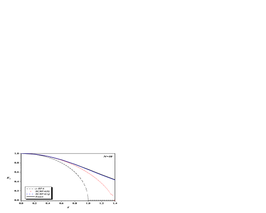
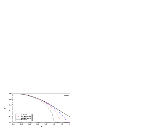
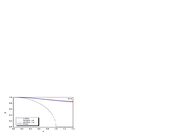
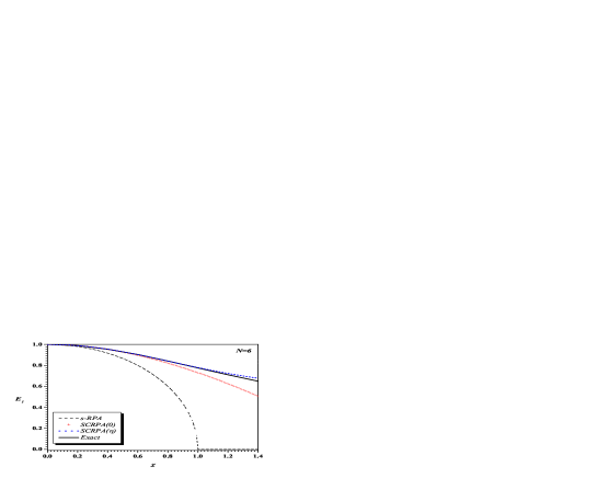
The solution for N=4𝑁4N=4, N=6𝑁6N=6 and N=10𝑁10N=10 can be obtained with the correlation functions given in the appendix (A). The results are shown in Figs 1, 2, 3, and 4. We see that SCRPA with η0𝜂0\eta\neq 0 (SCRPA(η𝜂\eta)) systematically and substantially improves over the η=0𝜂0\eta=0 case (SCRPA(0)) in the range χ<1𝜒1\chi<1. This fact shows that the extra correlations introduced in the excitation operator (12) improving the Pauli principle play an important role . In the range χ>1𝜒1\chi>1, ground and excited states become strongly mixed and SCRPA in the ’spherical’ basis deviates more and more from the exact solution. The good agreement of SCRPA(η)𝜂(\eta) with the exact solution also demonstrates that the convergence of our expansion scheme is fast. In future work it will be very interesting to apply our theory also to the symmetry broken regime.

IV Conclusions

In this work we have set up a Self-Consistent RPA (SCRPA) theory which is based on a fermionic many body vacuum. That is, we constructed a killing operator of the correlated vacuum |0exp[Z(2)]|HFket0𝑒𝑥𝑝delimited-[]superscript𝑍2ket𝐻𝐹|0\rangle\rightarrow exp[Z^{(2)}]|HF\rangle, with Z(2)superscript𝑍2Z^{(2)} a two body operator, see eq (9), (10) which also is the starting point of Coupled Cluster theory art5 . This killing operator consists of the usual ph𝑝ph RPA operator with, additionally, specific two body terms correcting for the Pauli principle. With this extended RPA operator, we develope the standard Equation of Motion technique and arrive at SCRPA equations of the usual mathematical structure. Since the extended RPA operator is not of the type of a canonical transformation between operators, the evaluation of the correlation functions contained in the RPA matrix in terms of the RPA amplitudes is not evident. We proposed a systematic expansion scheme in terms of higher and higher correlations functions (there may be room for improving this scheme) and applied it to the two level Lipkin model as a testing ground. It is found that the additional terms in the RPA operator systematically and substantially improve the results. We want to stress that once convergence is achieved with the mentioned expansion, the Pauli principle is fully respected, since our method is based on a fermionic many body ground state which is the vacuum to an (extended) RPA operator. In this way SCRPA which in the past suffered from the fact that it was based on a non existing vacuum is now put on grounds with more internal consistency. However, the practical success will depend on the convergence rate of our expansion scheme in more realistic situations. This is similar to the convergence rate of the hirarchy of hypernetted chain equations with Jastrow theory. In this work we only investigated the symmetry unbroken phase of the Lipkin model. The symmetry broken phase as well as other models for strongly interacting fermions shall be investigated in the future. On the formal level some questions still need to be considered also. The most important one is whether the Goldstone theorem when working in a symmetry broken phase still holds as in s-RPA. In particular this concerns the fullfillment of conservation laws, the appearence of a zero mode and the respect of Ward identities.

Acknowledgements.
We thank J. Dukelsky for very useful discussions. A critical reading of the manuscript and interesting comments from M. Holzmann are appreciated.

References

  • (1) P. Schuck, S. Ethofer, Nucl. Phys. A 212(1973)269; J. Dukelsky, G. Roepke, P. Schuck, Nucl. Phys. A 628(1998)17; D. S. Delion, P. Schuck, J. Dukelsky, Phys. Rev. C 72(2005)064305.
  • (2) J. P. Blaizot, G. Ripka Quantum Theory of Finite Systems , MIT Press (1986)
  • (3) P. Fulde, Electron Correlations in Molecules and Solids, Springer Series in Solid-State Sciences, Springer Verlag Berlin Heidelberg (1991)
  • (4) F. Gebhard, The Mott Metal Insulator Transition, Springer Tracts in Modern Physics, Vol. 137 (1997).
  • (5) R.F. Bishop, Theor. Chem. Acta 80(1991)95
  • (6) S. Takahara, M. Tohyama, P. Schuck, Phys. Rev. C 70(2004)057307; M. Tohyama, P.  Schuck, arXiv:1003.0246
  • (7) P. Ring, P. Schuck, The Nuclear Many–Body Problem, Springer Verlag, New York, (1980).
  • (8) J. Dukelsky, P. Schuck, Nucl. Phys. A 512(1990)466
  • (9) J.G. Hirsch, A. Mariano, J. Dukelsky, P. Schuck, Ann. Physics 296(2002)187
  • (10) P. Schuck, unpublished notes, 1987
  • (11) H. J. Lipkin, N. Meshkov, A.J. Glick, Nucl. Phys. 62(1965)197

Appendix A Correlation functions

In this Appendix, we list correlation functions to lowest non-trivial order as they are needed for the RPA calculation
Z|J^0|ZZ|Z=N21+2(N1)(N4)z21+2N(N1)z2quantum-operator-product𝑍subscript^𝐽0𝑍inner-product𝑍𝑍𝑁212𝑁1𝑁4superscript𝑧212𝑁𝑁1superscript𝑧2\frac{\langle Z|\hat{J}_{0}|Z\rangle}{\langle Z|Z\rangle}=-\frac{N}{2}\frac{1+2(N-1)(N-4)z^{2}}{1+2N(N-1)z^{2}}
Z|J^02|ZZ|Z=N4N+2(N1)(N4)2z21+2N(N1)z2quantum-operator-product𝑍superscriptsubscript^𝐽02𝑍inner-product𝑍𝑍𝑁4𝑁2𝑁1superscript𝑁42superscript𝑧212𝑁𝑁1superscript𝑧2\frac{\langle Z|\hat{J}_{0}^{2}|Z\rangle}{\langle Z|Z\rangle}=\frac{N}{4}\frac{N+2(N-1)(N-4)^{2}z^{2}}{1+2N(N-1)z^{2}}
Z|J^03|ZZ|Z=N8N2+2(N1)(N4)3z21+2N(N1)z2quantum-operator-product𝑍superscriptsubscript^𝐽03𝑍inner-product𝑍𝑍𝑁8superscript𝑁22𝑁1superscript𝑁43superscript𝑧212𝑁𝑁1superscript𝑧2\frac{\langle Z|\hat{J}_{0}^{3}|Z\rangle}{\langle Z|Z\rangle}=-\frac{N}{8}\frac{N^{2}+2(N-1)(N-4)^{3}z^{2}}{1+2N(N-1)z^{2}}
Z|J^2|ZZ|Z=Z|J^+2|ZZ|Z=2N(N1)z1+2N(N1)z2quantum-operator-product𝑍superscriptsubscript^𝐽2𝑍inner-product𝑍𝑍quantum-operator-product𝑍superscriptsubscript^𝐽2𝑍inner-product𝑍𝑍2𝑁𝑁1𝑧12𝑁𝑁1superscript𝑧2\frac{\langle Z|\hat{J}_{-}^{2}|Z\rangle}{\langle Z|Z\rangle}=\frac{\langle Z|\hat{J}_{+}^{2}|Z\rangle}{\langle Z|Z\rangle}=\frac{2N(N-1)z}{1+2N(N-1)z^{2}}
Z|J^+J^|ZZ|Z=4N(N1)2z21+2N(N1)z2quantum-operator-product𝑍subscript^𝐽subscript^𝐽𝑍inner-product𝑍𝑍4𝑁superscript𝑁12superscript𝑧212𝑁𝑁1superscript𝑧2\frac{\langle Z|\hat{J}_{+}\hat{J}_{-}|Z\rangle}{\langle Z|Z\rangle}=\frac{4N(N-1)^{2}z^{2}}{1+2N(N-1)z^{2}}
Z|J^+J^0J^|ZZ|Z=4N(N1)2(N2)z21+2N(N1)z2quantum-operator-product𝑍subscript^𝐽subscript^𝐽0subscript^𝐽𝑍inner-product𝑍𝑍4𝑁superscript𝑁12𝑁2superscript𝑧212𝑁𝑁1superscript𝑧2\frac{\langle Z|\hat{J}_{+}\hat{J}_{0}\hat{J}_{-}|Z\rangle}{\langle Z|Z\rangle}=-\frac{4N(N-1)^{2}(N-2)z^{2}}{1+2N(N-1)z^{2}}
Z|J^+2J^0|ZZ|Z=Z|J^0J^2|ZZ|Z=N2(N1)z1+2N(N1)z2quantum-operator-product𝑍superscriptsubscript^𝐽2subscript^𝐽0𝑍inner-product𝑍𝑍quantum-operator-product𝑍subscript^𝐽0superscriptsubscript^𝐽2𝑍inner-product𝑍𝑍superscript𝑁2𝑁1𝑧12𝑁𝑁1superscript𝑧2\frac{\langle Z|\hat{J}_{+}^{2}\hat{J}_{0}|Z\rangle}{\langle Z|Z\rangle}=\frac{\langle Z|\hat{J}_{0}\hat{J}_{-}^{2}|Z\rangle}{\langle Z|Z\rangle}=-\frac{N^{2}(N-1)z}{1+2N(N-1)z^{2}}
Z|J^+2J^02|ZZ|Z=Z|J^02J^2|ZZ|Z=12N3(N1)z1+2N(N1)z2quantum-operator-product𝑍superscriptsubscript^𝐽2superscriptsubscript^𝐽02𝑍inner-product𝑍𝑍quantum-operator-product𝑍superscriptsubscript^𝐽02superscriptsubscript^𝐽2𝑍inner-product𝑍𝑍12superscript𝑁3𝑁1𝑧12𝑁𝑁1superscript𝑧2\frac{\langle Z|\hat{J}_{+}^{2}\hat{J}_{0}^{2}|Z\rangle}{\langle Z|Z\rangle}=\frac{\langle Z|\hat{J}_{0}^{2}\hat{J}_{-}^{2}|Z\rangle}{\langle Z|Z\rangle}=\frac{1}{2}\frac{N^{3}(N-1)z}{1+2N(N-1)z^{2}}
Z|J^+3J^|ZZ|Z=Z|J^+J^3|ZZ|Z=0quantum-operator-product𝑍superscriptsubscript^𝐽3subscript^𝐽𝑍inner-product𝑍𝑍quantum-operator-product𝑍subscript^𝐽superscriptsubscript^𝐽3𝑍inner-product𝑍𝑍0\frac{\langle Z|\hat{J}_{+}^{3}\hat{J}_{-}|Z\rangle}{\langle Z|Z\rangle}=\frac{\langle Z|\hat{J}_{+}\hat{J}_{-}^{3}|Z\rangle}{\langle Z|Z\rangle}=0
Refer to caption
Figure 1: First excited state energy with s-RPA, SCRPA(0), SCRPA(η𝜂\eta), and exact solution for N=4𝑁4N=4 as a function of χ=V(N1)𝜒𝑉𝑁1\chi=V(N-1).
Refer to caption
Figure 2: Same as Fig. 1 but for N=6𝑁6N=6.
Refer to caption
Figure 3: Same as Fig. 1 but for N=10𝑁10N=10.
Refer to caption
Figure 4: Same as Fig. 1 but for N=20𝑁20N=20.