Copula Cosmology: Constructing a Likelihood Function

Abstract

To estimate cosmological parameters from a given dataset, we need to construct a likelihood function, which sometimes has a complicated functional form. We introduce the copula, a mathematical tool to construct an arbitrary multivariate distribution function from one-dimensional marginal distribution functions with any given dependence structure. It is shown that a likelihood function constructed by the so-called Gaussian copula can reproduce very well the $\displaystyle n$-dimensional probability distribution of the cosmic shear power spectrum obtained from a large number of ray-tracing simulations. This suggests that the Copula likelihood will be a powerful tool for future weak lensing analyses, instead of the conventional multivariate Gaussian likelihood.

I Introduction

Weak gravitational lensing by intervening large scale cosmic structures provides an excellent tool to probe the nature of dark matter and dark energy. The so-called “cosmic shear” signal has been successfully measured in various groups since 2000 (e.g. Bacon et al., 2000; Kaiser et al., 2000; Van Waerbeke et al., 2000; Wittman et al., 2000; Hamana et al., 2003; Jarvis et al., 2006; Semboloni et al., 2006; Fu et al., 2008; Schrabback et al., 2010; Semboloni et al., 2011). If systematic errors are well under control, the weak lensing has the highest potential to constrain the physical parameters in the equation of state governing the dark energy among the cosmological observations, such as type Ia supernovae, baryon acoustic oscillations, and number count of galaxy clusters (Albrecht et al., 2006, 2009; Joudaki et al., 2009).

A number of wide-field weak lensing surveys have been planned for this purpose, such as the Subaru Hyper Suprime-Cam Survey (Miyazaki et al., 2006), the Panoramic Survey Telescope & Rapid Response System (Pan-STARRS), the Dark Energy Survey (DES), the Large Synoptic Survey Telescope (LSST), the Joint Dark Energy Mission (JDEM) and Euclid (Refregier et al., 2010). It is expected that such wide-field weak lensing surveys will reduce statistical errors significantly compared to the past and ongoing surveys, because the number of observed galaxies increases proportional to the survey area. However, to make a maximal use of the full potential of planned weak lensing surveys for estimating cosmological parameters, it is of great importance to employ adequate statistical measures and methods for weak lensing. Particularly, one needs to take into account properly the correlations of the observables between different angular scales and redshifts, i.e. the covariances. Furthermore, we also need to use an appropriate likelihood function with given marginal distributions. If we do not use proper statistical measures and methods, or if we adopt an inaccurate covariance and/or a likelihood function, obtained results may be systematically biased (Hartlap et al., 2009; Ichiki et al., 2009).

For the cosmological parameter estimation, almost all previous authors used the $\displaystyle\chi^{2}$ method in weak lensing analyses (e.g. Hamana et al., 2003; Jarvis et al., 2006; Semboloni et al., 2006; Fu et al., 2008; Schrabback et al., 2010; Semboloni et al., 2011). However, it is found that the probability distribution function (PDF) of the weak lensing power spectrum is well approximated by the $\displaystyle\chi^{2}$ distribution though it has a larger positive tail than expected from the $\displaystyle\chi^{2}$ distribution Sato et al. (2009). The $\displaystyle\chi^{2}$ distribution deviates from the Gaussian distribution on large scales because the number of modes corresponding to the degree of freedom is very small. Meanwhile, the $\displaystyle\chi^{2}$ distribution approaches the Gaussian distribution at high $\displaystyle\ell$ due to the central limit theorem. We have to include this information accurately when we place constraints on the cosmological parameters.

If all of the marginal distributions are Gaussian distributed, it is straightforward to reconstruct the multivariate PDF, which is the so-called multivariate Gaussian PDF. However, it is not a trivial task to reconstruct the original multivariate PDF from general marginal distributions. There has been an infinite number of the degree of freedom in choosing the original PDF unless the dependence structure is specified. The copula provides us with a straightforward solution to this problem. The copula has been used in the field of mathematical finance, but not been widely used in the field of astronomy and cosmology, except only a few applications (Benabed et al., 2009; Jiang et al., 2009; Koen, 2009; Scherrer et al., 2010; Takeuchi, 2010). Hence, a copula may have a potential to open new fields of astronomy and cosmology.

In this paper, we construct a more plausible likelihood function using the Gaussian copula (hereafter “Copula likelihood”) than the multivariate Gaussian likelihood for the cosmic shear power spectrum. We show that the Copula likelihood well reproduces the $\displaystyle n$-dimensional probability distribution of the cosmic shear power spectrum estimated from 1000 realizations which is obtained from ray-tracing simulations performed by Sato et al. (2009). Cosmological parameters employed for our ray-tracing simulations are consistent with the WMAP 3-year results (Spergel et al., 2007). The detail descriptions of our ray-tracing simulations are summarized in Sato et al. (2009) (see also, Sato et al. (2010a)). In a companion paper (Sato et al., 2010b), we estimate the cosmological parameters using both the copula likelihood constructed by this paper and the Gaussian likelihood in order to evaluate how the difference between two likelihoods affects the parameter estimation.

II Formulation

The likelihood function is a central tool for any kind of parameter estimation. It is defined as a function of parameters in a given statistical model. The likelihood function $\displaystyle\mathcal{L}$ is related to the joint probability density function (JPDF) denoted by $\displaystyle f(\hat{x}_{1},\hat{x}_{2},\dots,\hat{x}_{n}\,|\,\theta)$ as

$$\mathcal{L}(\theta\,|\,\hat{x}_{1},\hat{x}_{2},\dots,\hat{x}_{n})=f(\hat{x}_{1},\hat{x}_{2},\dots,\hat{x}_{n}\,|\,\theta),$$ (1)

where $\displaystyle\hat{x}_{i}$ ($\displaystyle i=1,2,\dots,n$) are independent and identically-distributed observed variables and $\displaystyle\theta$ denotes model parameters. We will suppress the argument $\displaystyle\theta$ hereafter. Recall that the $\displaystyle n$-point cumulative distribution function (CDF), denoted by $\displaystyle F$, is defined as

$$F(\hat{x}_{1},\hat{x}_{2},\dots,\hat{x}_{n})=\int_{-\infty}^{\hat{x}_{1}}\int_{-\infty}^{\hat{x}_{2}}\dots\int_{-\infty}^{\hat{x}_{n}}f(x_{1},x_{2},\dots,x_{n}){\rm d}x_{1}{\rm d}x_{2}\dots\rm dx_{n},$$ (2)

and there is a following relation between JPDF and CDF:

$$f(\hat{x}_{1},\hat{x}_{2},\dots,\hat{x}_{n})=\frac{\partial^{n}F(\hat{x}_{1},\hat{x}_{2},\dots,\hat{x}_{n})}{\partial\hat{x}_{1}\partial\hat{x}_{2}\dots\partial\hat{x}_{n}}.$$ (3)

From the Sklar’s theorem (Sklar, 1959), we can obtain the following relation:

$${\rm Prob}(x_{1}\leq\hat{x}_{1},x_{2}\leq\hat{x}_{2},\dots,x_{n}\leq\hat{x}_{n})\equiv F(\hat{x}_{1},\hat{x}_{2},\dots,\hat{x}_{n})=C(F_{1}(\hat{x}_{1}),F_{2}(\hat{x}_{2}),\dots,F_{n}(\hat{x}_{n})),$$ (4)

where $\displaystyle C$ denotes the function called copula and $\displaystyle F_{i}$ denotes one-point CDF defined by

$$F_{i}(\hat{x}_{i})=\int_{-\infty}^{\hat{x}_{i}}f_{i}(x){\rm d}x\equiv u_{i}.$$ (5)

Therefore, the copula indicates how the one-point CDFs are jointed together to give the $\displaystyle n$-point CDF. A comprehensive proof of Sklar’s theorem and rigorous definition of a copula are found in Nelsen (2006); Takeuchi (2010). From the above relation, we can easily derive that $\displaystyle\hat{x}_{i}=F^{-1}_{i}(u_{i})$, and then derive the following relation,

$$C(u_{1},u_{2},\dots,u_{n})=F(F_{1}^{-1}(u_{1}),F_{2}^{-1}(u_{2}),\dots,F_{n}^{-1}(u_{n}))~{},$$ (6)

from Eq. (4). Differentiating Eq. (6) with Eq. (3) gives the density of copula $\displaystyle c$ as

$$c(u_{1},u_{2},\dots,u_{n})=\frac{\partial^{n}C(u_{1},u_{2},\dots,u_{n})}{\partial u_{1}\partial u_{2}\dots\partial u_{n}}=\frac{f(\hat{x}_{1},\hat{x}_{2},\dots,\hat{x}_{n})}{\displaystyle\prod_{i=1}^{n}f_{i}(\hat{x}_{i})},$$ (7)

where each $\displaystyle f_{i}$ is the marginal density function of the marginal CDF $\displaystyle F_{i}$. The JPDF can then be expressed as

$$f(\hat{x}_{1},\hat{x}_{2},\dots,\hat{x}_{n})=c(u_{1},u_{2},\dots,u_{n})\prod_{i=1}^{n}f_{i}(\hat{x}_{i}).$$ (8)

If the variables $\displaystyle x_{i}$ are independent of each other, $\displaystyle c=1$. In general, however, they are often correlated and $\displaystyle c$ shows their correlations as a function of one-point CDF of each stochastic variable.

III Gaussian Copula

In this section, we derive the Copula likelihood using a Gaussian copula which is more plausible than the multivariate Gaussian likelihood for the cosmic shear power spectrum. The multivariate Gaussian copula is the copula of the $\displaystyle n$-dimensional random vector that is normally distributed. This copula is expressed by

$$C(u_{1},u_{2},\dots,u_{n})\equiv\Phi\left(\Phi_{1}^{-1}(u_{1}),\Phi_{1}^{-1}(u_{2}),\dots,\Phi_{1}^{-1}(u_{n})\right).$$ (9)

Here one-point Gaussian CDF $\displaystyle\Phi_{1}$ is

$$\Phi_{1}(\hat{x}_{i})=\int_{-\infty}^{\hat{x}_{i}}\frac{1}{\sqrt{2\pi}\sigma_{i}}\exp\left(-\frac{(x-\mu_{i})^{2}}{2\sigma_{i}^{2}}\right){\rm d}x\equiv u_{i},$$ (10)

and $\displaystyle\Phi$ is $\displaystyle n$-point Gaussian CDF defined by

$$\Phi(\hat{x}_{1},\hat{x}_{2},\dots,\hat{x}_{n})=\int_{-\infty}^{\hat{x}_{1}}\int_{-\infty}^{\hat{x}_{2}}\dots\int_{-\infty}^{\hat{x}_{n}}\frac{1}{\sqrt{(2\pi)^{n}{\rm det(Cov)}}}\exp\left(-\frac{1}{2}(\boldsymbol{x}-\boldsymbol{\mu})^{\rm T}{\rm Cov}^{-1}(\boldsymbol{x}-\boldsymbol{\mu})\right){\rm d}x_{1}{\rm d}x_{2}\dots\rm dx_{n},$$ (11)

where we consider the $\displaystyle n$-point Gaussian CDF with mean $\displaystyle\boldsymbol{\mu}$ and $\displaystyle n\times{n}$ covariance matrix. $\displaystyle{\rm Cov}^{-1}$ shows the inverse covariance matrix. We define $\displaystyle\boldsymbol{\mu}\equiv(\mu_{1},\mu_{2},\dots,\mu_{n})$ and $\displaystyle\boldsymbol{x}\equiv(x_{1},x_{2},\dots,x_{n})$ and superscript ’T’ stands for the transpose of vector.

III.1 Gaussian PDF

Let us consider a two-variables case for simplicity. First consider the case that one-point PDF is Gaussian with $\displaystyle\sigma_{i}$ standard deviation and $\displaystyle\mu_{i}$ mean. In this case, the Gaussian copula is

$$\displaystyle C(\hat{x}_{1},\hat{x}_{2})=\Phi\left(\Phi_{1}^{-1}(\Phi_{1}(\hat{x}_{1})),\Phi_{1}^{-1}(\Phi_{1}(\hat{x}_{2}))\right),$$ (12)

$$\displaystyle\Phi(\hat{x}_{1},\hat{x}_{2})=\int_{-\infty}^{\hat{x}_{1}}\int_{-\infty}^{\hat{x}_{2}}\frac{1}{\sqrt{(2\pi)^{2}{\rm det(Cov)}}}\exp\left(-\frac{1}{2}(\boldsymbol{x}-\boldsymbol{\mu})^{\rm T}{\rm Cov}^{-1}(\boldsymbol{x}-\boldsymbol{\mu})\right){\rm d}x_{1}{\rm d}x_{2}\equiv\int_{-\infty}^{\hat{x}_{1}}\int_{-\infty}^{\hat{x}_{2}}\phi(x_{1},x_{2}){\rm d}x_{1}{\rm d}x_{2}.$$ (13)

From Eq. (7), we derive the density of copula as

$$\displaystyle c(u_{1},u_{2})=\frac{\partial\Phi(\hat{x}_{1},\hat{x}_{2})}{\partial u_{1}\partial u_{2}}=\frac{\partial^{2}\Phi}{\partial\hat{x}_{1}\partial\hat{x}_{2}}\frac{\partial\hat{x}_{1}}{\partial u_{1}}\frac{\partial\hat{x}_{2}}{\partial u_{2}}=\phi(\hat{x}_{1},\hat{x}_{2})\frac{\partial\hat{x}_{1}}{\partial u_{1}}\frac{\partial\hat{x}_{2}}{\partial u_{2}}.$$ (14)

By using

$$\displaystyle\frac{\partial u_{i}}{\partial\hat{x}_{i}}=\frac{1}{\sqrt{2\pi}\sigma_{i}}\exp\left(-\frac{(\hat{x}_{i}-\mu_{i})^{2}}{2\sigma_{i}^{2}}\right),$$ (15)

we finally obtain the density of copula as

$$\displaystyle c(u_{1},u_{2}) \displaystyle=\frac{\frac{1}{\sqrt{(2\pi)^{2}{\rm det(Cov)}}}\exp\left(-\frac{1}{2}(\boldsymbol{\hat{x}}-\boldsymbol{\mu})^{\rm T}{\rm Cov}^{-1}(\boldsymbol{\hat{x}}-\boldsymbol{\mu})\right)}{\frac{1}{\sqrt{2\pi}\sigma_{1}}\exp\left(-\frac{(\hat{x}_{1}-\mu_{1})^{2}}{2\sigma_{1}^{2}}\right)\frac{1}{\sqrt{2\pi}\sigma_{2}}\exp\left(-\frac{(\hat{x}_{2}-\mu_{2})^{2}}{2\sigma_{2}^{2}}\right)}$$

$$\displaystyle=\frac{\sigma_{1}\sigma_{2}}{\sqrt{\rm det(Cov)}}\exp\left[-\frac{1}{2}\left[(\boldsymbol{\hat{x}}-\boldsymbol{\mu})^{\rm T}({\rm Cov}^{-1}-(\boldsymbol{I\sigma^{2}})^{-1})(\boldsymbol{\hat{x}}-\boldsymbol{\mu})\right]\right],$$ (16)

where $\displaystyle\boldsymbol{I}$ stands for the identity matrix. Therefore, we can obtain the JPDF as

$$\displaystyle f(\hat{x}_{1},\hat{x}_{2}) \displaystyle=\frac{\sigma_{1}\sigma_{2}}{\sqrt{\rm det(Cov)}}\exp\left[-\frac{1}{2}\left[(\boldsymbol{\hat{x}}-\boldsymbol{\mu})^{\rm T}({\rm Cov}^{-1}-(\boldsymbol{I\sigma^{2}})^{-1})(\boldsymbol{\hat{x}}-\boldsymbol{\mu})\right]\right]\prod_{i=1}^{2}\frac{1}{\sqrt{2\pi}\sigma_{i}}\exp\left(-\frac{(\hat{x}_{i}-\mu_{i})^{2}}{2\sigma_{i}^{2}}\right)$$

$$\displaystyle=\frac{1}{\sqrt{(2\pi)^{2}{\rm det(Cov)}}}\exp\left(-\frac{1}{2}(\boldsymbol{\hat{x}}-\boldsymbol{\mu})^{\rm T}{\rm Cov}^{-1}(\boldsymbol{\hat{x}}-\boldsymbol{\mu})\right)$$ (17)

from Eq. (8). Therefore, the JPDF using the Gaussian copula with a Gaussian one-point PDF results in the multivariate Gaussian distribution, as expected.

III.2 Beyond Gaussian PDF

Now, let us consider the case in which a one-point PDF is not a Gaussian distribution but a general probability distribution $\displaystyle f_{i}$. In this case, the Gaussian copula is

$$C(\hat{x}_{1},\hat{x}_{2})=\Phi\left(\Phi_{1}^{-1}(F_{1}(\hat{x}_{1})),\Phi_{1}^{-1}(F_{2}(\hat{x}_{2}))\right),$$ (18)

where one-point CDF $\displaystyle F_{i}$ is

$$F_{i}(\hat{x}_{i})=\int_{-\infty}^{\hat{x}_{i}}f_{i}(x){\rm d}x\equiv u_{i}.$$ (19)

Defining $\displaystyle q_{i}$ as $\displaystyle q_{i}\equiv\Phi_{1}^{-1}(F_{i}(\hat{x}_{i}))=\Phi_{1}^{-1}(u_{i})$, we obtain the copula density from Eq. (18) as

$$c(u_{1},u_{2})=\frac{\partial^{2}\Phi(q_{1},q_{2})}{\partial u_{1}\partial u_{2}}=\frac{\partial^{2}\Phi}{\partial q_{1}\partial q_{2}}\frac{\partial q_{1}}{\partial u_{1}}\frac{\partial q_{2}}{\partial u_{2}},$$ (20)

where

$$\displaystyle\frac{\partial q_{i}}{\partial u_{i}}=\frac{\partial\Phi_{1}^{-1}(u_{i})}{\partial u_{i}}=\left(\frac{\partial\Phi_{1}(q_{i})}{\partial q_{i}}\right)^{-1}=\left(\frac{1}{\sqrt{2\pi}\sigma_{i}}\exp\left(-\frac{(q_{i}-\mu_{i})^{2}}{2\sigma_{i}^{2}}\right)\right)^{-1}.$$ (21)

We use a formula of the differential of the inverse function at the second equality of the above equation. By using Eq. (13) and Eq. (21), we rewrite Eq. (20) as

$$\displaystyle c(u_{1},u_{2})=\phi(q_{1},q_{2})\left(\frac{1}{\sqrt{2\pi}\sigma_{1}}\exp\left(-\frac{(q_{1}-\mu_{1})^{2}}{2\sigma_{1}^{2}}\right)\right)^{-1}\left(\frac{1}{\sqrt{2\pi}\sigma_{2}}\exp\left(-\frac{(q_{2}-\mu_{2})^{2}}{2\sigma_{2}^{2}}\right)\right)^{-1}.$$ (22)

From Eq. (8), we can easily calculate the JPDF as

$$\displaystyle f(\hat{x}_{1},\hat{x}_{2}) \displaystyle=\frac{1}{\sqrt{(2\pi)^{2}{\rm det(Cov)}}}\exp\left(-\frac{1}{2}(\boldsymbol{q}-\boldsymbol{\mu})^{\rm T}{\rm Cov}^{-1}(\boldsymbol{q}-\boldsymbol{\mu})\right)\left(\frac{1}{\sqrt{2\pi}\sigma_{1}}\exp\left(-\frac{(q_{1}-\mu_{1})^{2}}{2\sigma_{1}^{2}}\right)\right)^{-1}$$

$$\displaystyle\times\left(\frac{1}{\sqrt{2\pi}\sigma_{2}}\exp\left(-\frac{(q_{2}-\mu_{2})^{2}}{2\sigma_{2}^{2}}\right)\right)^{-1}f_{1}(\hat{x}_{1})f_{2}(\hat{x}_{2}).$$ (23)

We extend the above equation to the $\displaystyle n$-dimensional case and then finally obtain the $\displaystyle n$-dimensional JPDF as

$$\displaystyle f(\hat{x}_{1},\hat{x}_{2},\dots,\hat{x}_{n}) \displaystyle=\frac{1}{\sqrt{(2\pi)^{n}{\rm det(Cov)}}}\exp\left(-\frac{1}{2}(\boldsymbol{q}-\boldsymbol{\mu})^{\rm T}{\rm Cov}^{-1}(\boldsymbol{q}-\boldsymbol{\mu})\right)\prod_{i=1}^{n}\left(\frac{1}{\sqrt{2\pi}\sigma_{i}}\exp\left(-\frac{(q_{i}-\mu_{i})^{2}}{2\sigma_{i}^{2}}\right)\right)^{-1}f_{i}(\hat{x}_{i}).$$ (24)

If $\displaystyle f_{i}$ is Gaussian, $\displaystyle q_{i}$ becomes $\displaystyle\hat{x}_{i}$. In this case, we can see that $\displaystyle f(\hat{x}_{1},\hat{x}_{2},\dots,\hat{x}_{n})$ (Eq. 24) reduces to a multivariate Gaussian distribution. Therefore, when $\displaystyle f_{i}$ are not Gaussian PDFs, Eq. (24) carries the whole information on the correction to the Gaussian distribution.

Both in practice and from theoretical point of view (Takeuchi, 2000), it is more appropriate to work with the logarithm of the likelihood function, $\displaystyle\ln\mathcal{L}$, called log-likelihood. For example, the log-likelihood is used for the likelihood ratio test. The likelihood ratio test statistic is defined as twice the difference in these log-likelihoods with a minus sign. This quantity is also fundamental for the information statistics and information criterion theory (see, e.g. (Takeuchi, 2000) and references therein). From Eq. (24), this test statistic is derived as

$$\displaystyle-2\ln\mathcal{L}_{c}(\hat{x}_{1},\hat{x}_{2},\dots,\hat{x}_{n})=\sum_{i=1}^{n}\sum_{j=1}^{n}(q_{i}-\mu_{i}){\rm Cov}^{-1}(q_{j}-\mu_{j})-\sum_{i=1}^{n}\frac{(q_{i}-\mu_{i})^{2}}{\sigma_{i}^{2}}-2\sum_{i=1}^{n}\ln f_{i}(\hat{x}_{i}),$$ (25)

for a general probability distribution. For a Gaussian case it reduces to the well-known form

$$-2\ln\mathcal{L}_{g}(\hat{x}_{1},\hat{x}_{2},\dots,\hat{x}_{n})=\sum_{i=1}^{n}\sum_{j=1}^{n}(\hat{x}_{i}-\mu_{i}){\rm Cov}^{-1}(\hat{x}_{j}-\mu_{j}).$$ (26)

Here we abbreviate the irrelevant constant term in the above two equations.

Finally, we give the relation between $\displaystyle\hat{x}_{i}$ and $\displaystyle q_{i}$ because one has to calculate $\displaystyle q_{i}$ given $\displaystyle\hat{x}_{i}$. Since $\displaystyle\hat{x}_{i}$ is related to $\displaystyle u_{i}$ through Eq. (19), we have only to derive the relation between $\displaystyle u_{i}$ and $\displaystyle q_{i}$. From $\displaystyle q_{i}=\Phi_{1}^{-1}(u_{i})$, we get

$$u_{i}=\Phi_{1}(q_{i})=\int_{-\infty}^{q_{i}}\frac{1}{\sqrt{2\pi}\sigma_{i}}\exp\left(-\frac{(x-\mu_{i})^{2}}{2\sigma_{i}^{2}}\right){\rm d}x.$$ (27)

We change the variable $\displaystyle x$ to $\displaystyle y=(x-\mu_{i})/\sigma_{i}$ and then obtain

$$u_{i}=\frac{1}{\sqrt{2\pi}}\int_{-\infty}^{\frac{q_{i}-\mu_{i}}{\sigma_{i}}}\exp\left(-\frac{y^{2}}{2}\right){\rm d}{y}.$$ (28)

At a first glance, we can recognize this equation as $\displaystyle u_{i}=\Psi_{1}\left(\frac{q_{i}-\mu_{i}}{\sigma_{i}}\right)$, where $\displaystyle\Psi_{1}$ is the cumulative standard normal distribution. We can obtain the relation between $\displaystyle u_{i}$ and $\displaystyle q_{i}$ as

$$\frac{q_{i}-\mu_{i}}{\sigma_{i}}=\Psi_{1}^{-1}(u_{i})\Leftrightarrow q_{i}=\sigma_{i}\Psi_{1}^{-1}(u_{i})+\mu_{i}.$$ (29)

IV Result and Discussion

In this section, we investigate whether the Copula likelihood (Eq. 25) reproduces the $\displaystyle n$-dimensional JPDF obtained from ray-tracing simulations performed by Sato et al. (2009). We then compare the shape of the Copula likelihood with that of the Gaussian likelihood and how the Copula likelihood is statistically better than the Gaussian likelihood. In our application, the observed variables $\displaystyle\hat{x}_{i}$ are the binned convergence power spectra $\displaystyle\hat{P}_{\kappa}(\ell_{i})$, which are estimated from each realization. We estimate it for an assumed bin width $\displaystyle\Delta\ln{\ell}$. Throughout this paper, we employ the bin width $\displaystyle\Delta\ln\ell=0.3$ and assume that the single source redshift distribution, i.e. all lensed galaxies lie at $\displaystyle z_{s}=1.0$ and we do not consider intrinsic ellipticity dispersion $\displaystyle\sigma_{\epsilon}$. In our ray-tracing simulations, the survey area is set as $\displaystyle\Omega_{\rm s}=25$ deg². Therefore the fundamental mode of our ray-tracing simulations is at the multipole $\displaystyle\ell_{f}=72$. We take 13 bins for our likelihood analysis. Therefore, we cover the multipole range from $\displaystyle\ell_{f}=72$ to $\displaystyle\ell_{\rm max}=2635$. We call the convergence power spectrum estimated at bin $\displaystyle i$ as “bin $\displaystyle i$ power”.

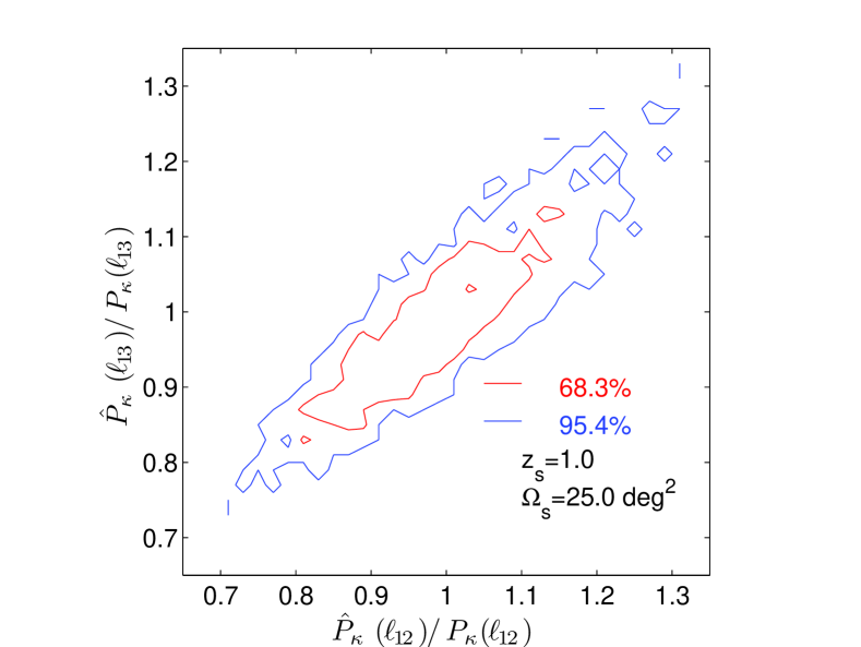
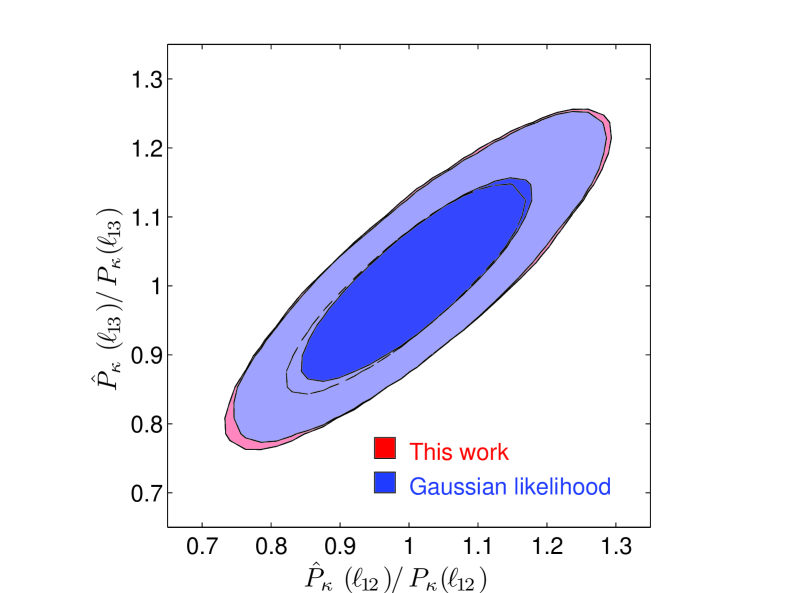
The left panel of Fig. 1 shows the two-dimensional JPDF between bin 1 power and bin 2 power from 1000 realizations of ray-tracing simulations. The one-point PDF is normalized so that the mean power spectrum is equal to unity. The red solid and blue solid contours show the 1$\displaystyle\sigma$ and 2$\displaystyle\sigma$ confidence level (CL) regions, respectively. In the right panel of Fig. 1, the blue and red contours show two-dimensional marginalized 1$\displaystyle\sigma$ and 2$\displaystyle\sigma$ confidence regions on the bin 1 power and bin 2 power plane, which are derived from the Gaussian likelihood (Eq. 26) and Copula likelihood (Eq. 25), respectively. One can clearly see that the Copula likelihood model reproduces the simulation data (left panel of Fig. 1) much better than the Gaussian likelihood model, as discussed below.

In our Copula likelihood model, we have chosen a $\displaystyle\chi^{2}$ distribution for a general one-point probability distribution $\displaystyle f_{i}$. This is a nice choice because the one-point PDF of convergence power spectrum is fairly well described by a $\displaystyle\chi^{2}$ distribution where the mean and variance are $\displaystyle P_{\kappa}(\ell_{i})=\langle{\hat{P}_{\kappa}(\ell_{i})}\rangle$ and $\displaystyle\sigma^{2}(\ell_{i})=\langle\hat{P}_{\kappa}(\ell_{i})^{2}\rangle-P_{\kappa}(\ell_{i})^{2}$, respectively (see Sato et al., 2009). From Takahashi et al. (2009), this $\displaystyle\chi^{2}$ distribution is shown as

$$f_{\chi^{2}}(\hat{P}_{\kappa}(\ell_{i}))=\frac{\hat{P}_{\kappa}(\ell_{i})^{\Upsilon-1}}{\Gamma(\Upsilon)}\left(\Upsilon\frac{e^{-\hat{P}_{\kappa}(\ell_{i})/P_{\kappa}(\ell_{i})}}{P_{\kappa}(\ell_{i})}\right)^{\Upsilon},$$ (30)

for $\displaystyle\hat{P}_{\kappa}(\ell_{i})>0$ and $\displaystyle f_{\chi^{2}}=0$ for $\displaystyle\hat{P}_{\kappa}(\ell_{i})\leq 0$. Here, $\displaystyle\Gamma(x)$ is the gamma function and we define $\displaystyle\Upsilon\equiv{P_{\kappa}(\ell_{i})^{2}/\sigma^{2}(\ell_{i})}$ which corresponds to the number of independent modes. The covariance matrix is also estimated from the simulation.

In order to obtain these likelihood contours, we employed the Markov Chain Monte Carlo method (Lewis and Bridle, 2002). Assuming flat priors for bin $\displaystyle i$ powers, we explored bin $\displaystyle i$ power estimations in the multidimensional space (i.e. 13 dimensional space in this case). Eight parallel chains are computed and the convergence test is made based on the Gelman and Rubin statistics called “$\displaystyle R-1$” statistics (Gelman and Rubin, 1992). Each of our chains typically has 400,000 points and $\displaystyle R-1<0.05$ in both models.

We can see that the results between our Copula likelihood function (red contours) and the Gaussian likelihood (blue contours) are very different. The difference mainly comes from the one-point PDF, which is taken as a $\displaystyle\chi^{2}$ distribution or a Gaussian distribution. The $\displaystyle\chi^{2}$ distribution denoted by Eq. (30) deviates from the Gaussian distribution on large scales, such as a case considered in Fig. 1, because the number of modes corresponding to the degrees of freedom is very small. We can also see that our likelihood function well reproduces the results from ray-tracing simulations than the Gaussian likelihood. In particular, the results of our Copula likelihood function capture the feature that the value which takes the maximum probability deviates from the mean value. The values at which the Copula likelihood takes its maximum are $\displaystyle(0.619,0.241)$ at bin 1 and bin 2.

Figure 1: Left panel: Two-dimensional JPDF between convergence power spectrum estimated at bin 1 and bin 2 among 1000 realizations obtained from ray-tracing simulations. The bin 1 and bin 2 correspond to multipole $\displaystyle\ell=72$ and $\displaystyle\ell=97$, respectively. The one-point PDF is normalized so that the mean convergence power spectrum estimated at each bin gives unity. The red solid and blue solid contours show 1$\displaystyle\sigma$ and 2$\displaystyle\sigma$ CL, respectively. Right panel: Two-dimensional marginalized constraints on convergence power spectrum estimated at bin 1 and bin 2. The red and blue contours show the marginalized constraints (1$\displaystyle\sigma$ and 2$\displaystyle\sigma$ CL) obtained by Eq. (25) based on the Gaussian copula model and Gaussian likelihood of Eq. (26), respectively.

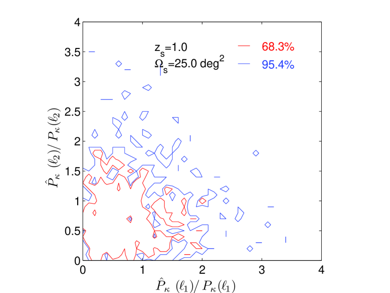
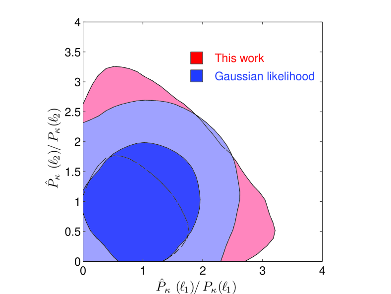
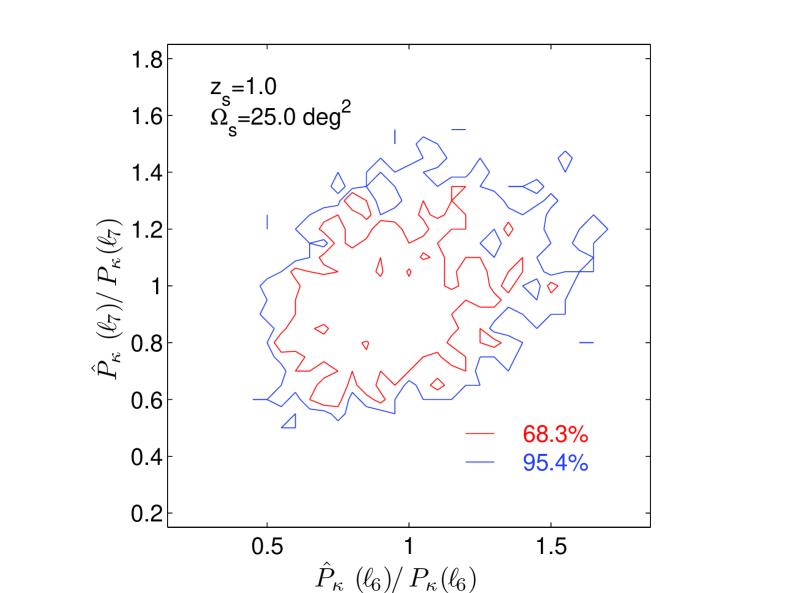
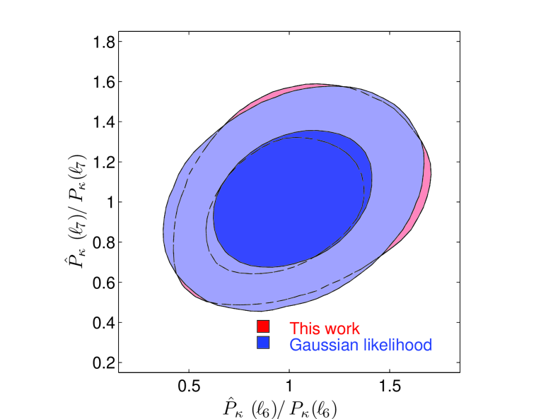
Figure 2 is same as Fig. 1, but results from bin 6 power and bin 7 power. The bin 6 and bin 7 correspond to the multipoles $\displaystyle\ell=323$ and $\displaystyle\ell=436$, respectively. The results from our likelihood are similar to the results from the Gaussian likelihood, because the $\displaystyle\chi^{2}$ distribution approaches Gaussian distribution at these scales. However, we can see the small deviation from each mean value between the results obtained from the two likelihoods.

Figure 3 is also the same as Fig. 1, but results from bin 12 power and bin 13 power. The bin 12 and bin 13 correspond to the multipoles $\displaystyle\ell=1952$ and $\displaystyle\ell=2635$, respectively. The contours from the copula likelihood are nearly identical to those from the Gaussian likelihood, because the $\displaystyle\chi^{2}$ distribution approaches to Gaussian distribution at these small scales due to the central limit theorem. We can see a positive strong correlation which is mainly attributed to the fact that the nonlinear gravitational evolution causes the non-Gaussian contribution and correlations between different multipole bins (e.g., see in Fig. 7 in (Sato et al., 2009)).

Figure 2: Same as Fig. 1, but convergence power spectrum is estimated at bin 6 and bin 7.

Figure 3: Same as Fig. 1, but convergence power spectrum is estimated at bin 12 and bin 13.

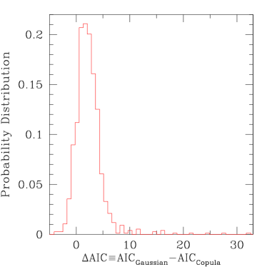
To confirm a much better reliability of our Copula likelihood, we examine how the Copula likelihood is statistically better relative to the Gaussian likelihood based on the information criterion theory. We use the Akaike Information Criterion (AIC) (Akaike, 1974; Takeuchi, 2000; Spiegelhalter et al., 2002) to evaluate which model is more preferable. The AIC is defined as

$${\rm AIC}\equiv-2\ln\mathcal{L}_{\rm max}+2k,$$ (31)

where $\displaystyle\mathcal{L}_{\rm max}$ is the maximum likelihood achievable by the model under a certain dataset, and $\displaystyle k$ is the number of free parameters of the model. In the present analysis $\displaystyle\mathcal{L}_{\rm max}$ is directly obtained by substituting $\displaystyle\hat{P}_{\kappa}(\ell_{i})$ into Eqs. (25) and (26) at each realization, because model parameters have been already fixed to give the maximum probability for the 1000 realized simulation data. The meaning of the AIC is clearly understood as an extension of the maximum likelihood method. An explanation for astronomers can be found in (Takeuchi, 2000) and there are also useful applications of the AIC in their paper. Using the AIC enables us to compare the goodness of a certain model with that of another type directly. Figure 4 shows the PDF of the AIC difference, $\displaystyle\Delta{\rm AIC}\equiv{\rm AIC}_{\rm Gaussian}-{\rm AIC}_{\rm Copula}$ among 1000 realizations. We see that the AIC is significantly reduced by the Copula likelihood (positive $\displaystyle\Delta{\rm AIC}$) for the vast majority of the realizations. This means that the Copula likelihood function represents the distribution of the convergence power spectra from Monte Carlo simulations better than the Gaussian likelihood one. We estimate that the mean value of the AIC difference is 2.35. Some rough rules of thumb are available and useful for estimation of the goodness of models. As shown in (Burnham and Anderson, 2002), the mean value of the AIC difference we have estimated is regarded as Considerably less which means the evidence to support the Gaussian likelihood is considerably less than the Copula likelihood. Therefore we can conclude that our Copula likelihood is strongly favored compared to the Gaussian likelihood for cosmic shear power spectrum.

Finally, we discuss how the difference between the two likelihoods affects the cosmological parameter estimation, paying attention to the number of bins. Since weak lensing power spectra are expected to be very smooth in $\displaystyle\ell$, it is very likely that little information is lost by binning as long as the bins are narrow compared to the width of any features. If we consider an observation over the sky coverage $\displaystyle f_{\rm sky}$ ($\displaystyle f_{\rm sky}=\Omega_{\rm s}/4\pi$) with useful signal at $\displaystyle\ell_{f}\lower 2.15277pt\hbox{$\displaystyle\;\buildrel<\over{\sim}\;$}\ell\lower 2.15277pt\hbox{$\displaystyle\;\buildrel<\over{\sim}\;$}\ell_{\rm max}$, the total number of modes one can obtain is estimated to be $\displaystyle n_{t}\sim f_{\rm sky}(\ell_{\rm max}^{2}-\ell_{f}^{2})$. If the number of bins is small enough, the distribution of the power at each bin can be approximated by a Gaussian because a sufficient number of modes are in that bin. As is shown in (Hamimeche and Lewis, 2008) if the number of bins satisfies a condition $\displaystyle n_{b}\ll f_{\rm sky}^{1/2}\ell_{\rm max}$ assuming $\displaystyle\ell_{\rm max}^{2}\gg\ell_{f}^{2}$, the Gaussian approximation for the one-point PDF at each bin becomes very good. In that case one can use the multivariate Gaussian likelihood in order to estimate the cosmological parameters, which will simplify the parameter estimation analysis. Now let us apply this argument to our examples. In our example with $\displaystyle f_{\rm sky}=6.25\times 10^{-4}$ and $\displaystyle\ell_{\rm max}\sim 1000$, the square root of the total number of the modes is $\displaystyle n_{t}\sim f_{\rm sky}^{1/2}\ell_{\rm max}=25$. This number is not so large compared to the number of bins, i.e., $\displaystyle n_{b}=13$. Therefore, in this case an accurate likelihood function should be used in order to get unbiased cosmological parameter constraints, instead of the conventional multivariate Gaussian likelihood (see, Sato et al., 2010b). Meanwhile, if we consider a future type survey which has $\displaystyle f_{\rm sky}=0.05$ and $\displaystyle\ell_{\rm max}\sim 1000$ with the same number of bins, the square root of the total number of the modes is $\displaystyle f_{\rm sky}^{1/2}\ell_{\rm max}=224$ which is much larger than the number of bins. Then, the Gaussian approximation could be fine in this case (Sato et al., 2010b) . Note, however, that Gaussian approximation may be violated by natural binning which has optimal $\displaystyle\ell$ resolution, regardless of how $\displaystyle\ell_{\rm max}$ value is. Therefore, we suggest the Copula likelihood should be used when an optimal binning is done to keep the cosmological information as much as possible. The impact of the difference between the two likelihoods on cosmological parameter estimations is illustrated and discussed carefully in a companion paper (Sato et al., 2010b).

Figure 4: Probability distribution of the Akaike Information Criterion (AIC) difference between the Copula likelihood (Eq. 25) and the Gaussian likelihood (Eq. 26), among 1000 realizations.

V Conclusion

It has been becoming an important issue to obtain not only accurate statistics such as a power spectrum and covariance matrix but also an accurate likelihood function for the precision cosmology. In this work, we introduced a statistical tool called a copula into cosmology in a rather pedagogical way. The copula is a function to generate an $\displaystyle n$-point CDF from the given one-point CDFs and prescribed dependence structure of variables. We then applied the copula to the cosmic convergence power spectrum estimated from 1000 realizations obtained from ray-tracing simulations generated by (Sato et al., 2009).

By taking into account the fact that the one-point PDF of the convergence power spectrum is well approximated by $\displaystyle\chi^{2}$ distribution, we showed that the Gaussian copula can reproduce the $\displaystyle n$-dimensional shape of the likelihood function of the convergence power spectrum better than the multivariate Gaussian likelihood, for the simulated 13-binned data expected from the assumed survey area of $\displaystyle\Omega_{\rm s}=25$ deg². This is a main result of the present paper. The differences between the two likelihood models become significant at lowest multipole bins.

The deviation from the multivariate Gaussian will heavily depend on the width of the binning. We discussed that a sufficiently sparse binning will make it possible to use a multivariate Gaussian likelihood for the future cosmic shear survey. However, if one makes an optimal binning ($\displaystyle\Delta\ell\sim 1$) to keep the information as much as possible, non-Gaussian corrections will become important. In this case the copula will provide us an appropriate likelihood function in a convenient way by relating the one-point CDFs to the $\displaystyle n$-point CDF.