A conformal invariant growth model

Abstract

We present a one-parameter extension of the raise and peel one-dimensional growth model. The model is defined in the configuration space of Dyck (RSOS) paths. Tiles from a rarefied gas hit the interface and change its shape. The adsorption rates are local but the desorption rates are non-local, they depend not only on the cluster hit by the tile but also on the total number of peaks (local maxima) belonging to all the clusters of the configuration. The domain of the parameter is determined by the condition that the rates are non-negative. In the finite-size scaling limit, the model is conformal invariant in the whole open domain. The parameter appears in the sound velocity only. At the boundary of the domain, the stationary state is an adsorbing state and conformal invariance is lost. The model allows to check the universality of nonlocal observables in the raise and peel model. An example is given.

1 Introduction

In the study of adsorption-desorption (deposition-evaporation) processes on a planar surface, the Edwards-Wilkinson [1] and the Kardar-Parisi-Zhang [2] growth models have been extensively researched. The corresponding dynamical critical exponents $z$ being equal to 2 respectively 3/2. Recently the raise and peel model (RPM) was introduced [3]. In this one parameter dependent model, adsorption is local but desorption is not (the interface is ”peeled”). When the parameter is changed in the critical domain, $z$ changes too, varying from $z=1$ to zero. The model was extended to contain sources at the boundaries [4] and defects [5]. The RPM was also used to check various estimators in information theory [6].

If one fixes the value of the parameter such that $z=1$, the model has magical properties. The system has a space-time symmetry (conformal invariance) and the stationary state probability distribution function (PDF) has fascinating combinatorial properties [7] being related to a two-dimensional equilibrium system [8]. This is also the single case where the system is integrable.

In the present paper we will consider the RPM at the conformal invariant point only. With a few exceptions, it is not yet known which characteristics of the stationary state are universal and the time-dependent properties of the interface are by and large, uncharted territory. The aim of this paper is to introduce a new model, dependent on a parameter $p$, which is in the same universality class as the RPM. This implies that in the finite-size scaling limit the models coincide for the whole range of values of $p$. It turns out that in this limit, the single difference between the models is the value of the sound velocity $v_{s}(p)$ which is a function of $p$. Since the models are not local, finding models belonging to the same universality class is not an obvious matter.

For reasons which will be apparent later on, we call the new model the peak adjusted raise and peel model (PARPM), it is presented in Section 2. Except for $p=1$, the rates are dependent on the system-size $L$ and on $p$. The PARPM for $p\neq 1$ is not integrable and therefore all the results we have are based on Monte Carlo simulations on large lattices. In the stationary states, the PDF’s have no magic properties.

In Section 3 we show that, in the finite-size scaling limit the density of contact points is independent of the parameter $p$. This observation is important since for $p=1$ one recovers the RPM and for this case, the density of contact points is known exactly (this knowledge is based on conformal field theory and combinatorics [4]).

We next examine the time dependence of the average number of clusters for various lattices sizes using the Family-Vicsek analysis [9]. The large time behavior of the density is given by a few levels of the spectrum of the evolution operator (Hamiltonian) and it is well understood for $p=1$. We have observed that by a rescaling of the time, which implies changing the sound velocity $v_{s}(p)$ as a function of $p$, one obtains the same finite-size scaling function of $tv_{s}(p)/Lv_{s}(1)$ for all values of $p$ ($L$ is the system size). In order to check that this picture is correct, we have done a finite-size scaling analysis of the spectrum of the Hamiltonians and found the same values for $v_{s}(p)$ as the ones determined in obtaining the Family-Vicsek function.

The sound velocity stays finite for $p$ in the interval $0\leq p<2$ and vanishes for $p=2$ (the procedure how to take the limit $p\to 2$ is explained in the text). At $p=2$ the stationary state is an adsorbing state and conformal invariance is lost.

We believe that the results mentioned above are a clear demonstration that the PARPM is in the same universality class as the RPM. These observations opens the possibility to look for other universal quantities than those already considered in the study of the RPM. Since the models are not local, there is no recipe to find them. We will show that the average density of sites where desorption does not take place is universal: for large values of $L$, its value is independent of $p$.

Our conclusions are presented in Section 4.

2 Description of the peak adjusted raise and peel model

We consider an open one-dimensional system with $L+1$ sites ($L$ even). A Dyck path (restricted solid-on-solid (RSOS) configuration) is defined as follows. We attach to each site $i$ non-negative integer heights $h_{i}$ which obey RSOS rules:

$$h_{i+1}-h_{i}=\pm 1,\quad h_{0}=h_{L}=0\quad(i=0,1,\ldots,L-1).$$ (2.1)

There are

$$Z(L)=L!/(L/2)!(L/2+1)!$$ (2.2)

configurations of this kind. If $h_{j}=0$ at the site $j$ one has a contact point. Between two consecutive contact points one has a cluster. There are four contact points and three clusters in Fig. 1.

Figure 1: An example of a Dyck path for L = 14. There are four contact points and three clusters. The substrate profile is shown in blue.

A Dyck path is seen as an interface separating a film of tilted tiles deposited on a substrate from a rarefied gas of tiles (see Fig. 2). The stochastic processes in discrete time has two steps:

a) Sequential updating. With a probability $P(i)$ a tile hits the site $i=1,\ldots,L-1$ ($\sum_{i}P(i)=1$). In the RPM, $P(i)$ is chosen uniform: $P(i)=P=1/(L-1)$. In the PARPM, this is not longer the case. For a given configuration (there are $Z(L)$ of them), all the peaks are hit with the same probability $R_{p}=p/(L-1)$ ($p$ is a non-negative parameter), all the other sites are hit with the same probability $Q_{c}=q_{c}/(L-1)$ where

$$q_{c}=(L-1-pn_{c})/(L-1-n_{c}),\quad c=1,2,\ldots,Z(L).$$ (2.3)

Here $n_{c}$ is the number of peaks in the configuration (labelled by $c$). $q_{c}$ depends on the configuration $c$ (with $L$ sites and $n_{c}$ peaks) and on the parameter $p$. Obviously:

$$n_{c}R_{p}+(L-1-n_{c})Q_{c}=1.$$ (2.4)

b) Effects of a hit by a tile. The consequence of the hit on a configuration is the same as in the RPM at the conformal invariant point.

Figure 2: Example of a configuration with 4 peaks of the PARPM for L = 18. Depending on the position where the tilted tiles reach the interface, several distinct processes occur (see the text).

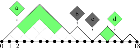
Depending of the slope $s_{i}=(h_{i+1}-h_{i-1})/2$ at the site $i$, the following processes can occur:

1) $s_{i}=0$ and $h_{i}>h_{i-1}$ (tile $b$ in Fig 2). The tile hits a peak and is reflected.

2) $s_{i}=0$ and $h_{i}<h_{i-1}$ (tile $c$ in Fig. 2) . The tile hits a local minimum and is adsorbed ($h_{i}\rightarrow h_{i}+2$).

3) $s_{i}=1$ (tile $a$ in fig. 2). The tile is reflected after triggering the desorption ($h_{j}\rightarrow h_{j}-2$) of a layer of $b-1$ tiles from the segment $\{j=i+1,\ldots,i+b-1\}$ where $h_{j}>h_{i}=h_{i+b}$.

4) $s_{i}=-1$ (tile $d$ in Fig. 2). The tile is reflected after triggering the desorption ($h_{j}\rightarrow h_{j}-2$) of a layer of $b-1$ tiles belonging to the segment $\{j=i-b+1,\ldots,i-1\}$ where $h_{j}>h_{i}=h_{i-b}$.

The continuous time evolution of a system composed by the states $a=1,2,\ldots,Z(L)$ with probabilities $P_{a}(t)$ is given by a master equation that can be interpreted as an imaginary time Schrödinger equation:

$$\frac{d}{dt}P_{a}(t)=-\sum_{b}H_{a,b}P_{b}(t),$$ (2.5)

where the Hamiltonian $H$ is an $Z(L)\times Z(L)$ intensity matrix: $H_{a,b}$ non positive ($a\neq b$) and $\sum_{a}H_{a,b}=0$. $-H_{a,b}$ is the rate for the transition $|b\rangle\rightarrow|a\rangle$. The ground-state wavefunction of the system $|0\rangle$, $H|0\rangle=0$, gives the probabilities in the stationary state:

$$|0\rangle=\sum_{a}P_{a}|a\rangle,\;\;\;\;\;\;P_{a}=\lim_{t\to\infty}P_{a}(t).$$ (2.6)

In order to go from the discrete time description of the stochastic model to the continuous time limit, we take $\Delta t=1/(L-1)$ and

$$H_{ac}=-r_{ac}q_{c}\quad(c\neq a),$$ (2.7)

where $r_{ac}$ are the rates of the RPM and $q_{c}$ is given by Eq. (2.3). The probabilities $R_{p}$ don’t enter in (2.5) since in the RPM when a tile hits a peak, the tile is reflected and the configuration stays unchanged. Notice that through the $q_{c}$’s the matrix elements of the Hamiltonian depend on the size of the system and the numbers of peaks $n_{c}$ of the configurations.

As an example, we consider a system with $L=6$. In this case there are 5 configurations shown in Fig. 3. The Hamiltonian is given by:

Figure 3: The five Dyck path configurations for $L=6$

.

$$H=-\left(\begin{array}[]{c|rrrrr}&|1\rangle&|2\rangle&|3\rangle&|4\rangle&|5\rangle\\ \hline\cr\langle 1|&-5+3p&2[(5-2p)/3]&2[(5-2p)/3]&0&2[(5-p)/4]\\ \langle 2|&(5-3p)/2&-5+2p&0&(5-2p)/3&0\\ \langle 3|&(5-3p)/2&0&-5+2p&(5-2p)/3&0\\ \langle 4|&0&(5-2p)/3&(5-2p)/3&-5+2p&2[(5-p)/4]\\ \langle 5|&0&0&0&(5-2p)/3&-5+p\end{array}\right).$$ (2.14)

If in (2.14) one takes $p=1$, one recovers the Hamiltonian of the RPM for $L=6$ [10].

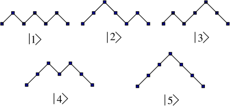
The unnormalized PDF in the stationary state is given by the eigenvector corresponding to the eigenvalue zero of (5):

$$\left|{\frac{11(5-p)}{2(5-3p)},\frac{15(5-p)}{4(5-2p)},\frac{15(5-p)}{4(5-2p)},\frac{3(5-p)}{5-2p},1}\right>.$$ (2.15)

Except for $p=1$ [3], there are no nice combinatorial properties of the components in (2.15) for rational values of $p$. This was checked also for larger lattices.

Let us observe that if $p=5/3$, the configuration $|1\rangle$ which corresponds to the substrate, becomes an adsorptive state. This phenomenon is general. For an arbitrary value of $L$, the substrate has $n_{p}=L/2$ peaks therefore, using (2.3) we conclude that for $p=2(L-1)/L$, the substrate is an adsorbing state. For larger values of $p$, one obtains negative rates, which gives

$$0\leq p<2(L-1)/L$$ (2.16)

as the domain of $p$.

3 Conformal invariance in the PARPM

We have invented the PARPM expecting for $p\neq 1$ different properties than those observed. It came as a surprise that the PARPM belonged to the same universality class as the RPM. Let us first show that in the stationary state the density of contact points $g(x,L)$ ($x$ is the distance to the origin and $L$ the size of the system) is, in the finite-size scaling limit ($x>>1$, $L>>1$ but $x/L$ fixed), independent of $p$ and equal to

$$g(x,L)=C\left(\frac{L}{\pi}\sin(\pi x/L)\right)^{-1/3},$$ (3.1)

where

$$C=-\frac{\sqrt{3}}{6\pi^{\frac{5}{6}}}\Gamma(-1/6)=0.753149...\quad.$$ (3.2)

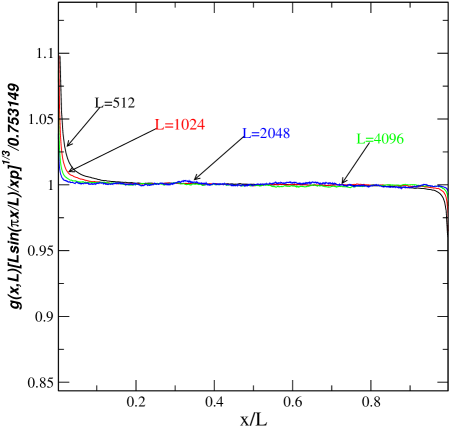
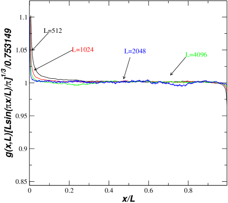
This expression is exact for $p=1$ [4] and its functional form (not the constant $C$ which is obtained using combinatorics) is a result of conformal invariance. In Figs. 4 and 5 we show the $x/L$ dependence of the densities of contact points divided by the expression (3.1), as obtained from Monte Carlo simulations for two extreme values of $p$ (0.01 and 1.99) and various lattices sizes. Similar calculations, done for other values of $p$, give the same result: in the finite-size limit, the density of contact points is independent of $p$. From the data collapse seen in the figures, we conclude that the first test of universality is successful.

Figure 4: The density of contact points $g(x,L)$ divided by (3.1) for $p=0.01$ and lattices sizes $L=510,1024,2048$ and 4096.

Figure 5: Same as Fig. 4 for $p=1.99$.

Let us consider now space-time properties of the model. One starts at $t=0$ with the configuration describing the substrate and we look at the average number of clusters $k(t,L)$ as a function of time and lattice sizes. In order to determine the dynamical critical exponent $z$ for various values of $p$, we compute the Family-Vicsek scaling function [9]

$$K(t,L)=k(t,L)/k(L)-1,$$ (3.3)

where $k(L)$ is the average number of clusters in the stationary state. In the finite-size scaling limit one expects

$$K(t,L)=~{}K(t/L^{z}).$$ (3.4)

Figure 6: The Family-Vicsek scaling function $K(t,L)$ as a function of $t/L$ for $p=0.1,0.5,1,1.5$ and 1.9 and lattice sizes $L=1024,2048,4096$ and 8192.

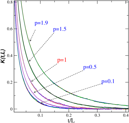
In Fig. 6 we show the results of the Monte Carlo simulations. For each value of $p$ one has data collapse which implies $z=1$ for all the values of $p$ (see (3.4)). One now show that by a change of the time scale, one can get the different scaling functions in Fig. 6 to coincide. Let us keep in mind that in a conformal invariant theory, the finite-size scaling limit of the spectrum of the Hamiltonian has the following behavior (the ground-state eigenvalue $E_{0}$ is equal to zero for a stochastic process):

$$\lim_{L\to\infty}E_{i}(L)=\pi v_{s}x_{i}/L,\quad i=0,1,2,\ldots$$ (3.5)

where $v_{s}$ is the sound velocity and $x_{i}$ are critical exponents. This implies that

$$K(t/L)=\sum_{i}C_{i}\exp(-E_{i}t)=\sum_{i}C_{i}\exp(-\pi v_{s}x_{i}t/L),$$ (3.6)

where the constants $C_{i}$ depend on the initial conditions. As discussed in [10], for $p=1$ one has:

$$v_{s}(1)=\frac{3}{2}\sqrt{3},\quad x_{1}=2,\quad x_{2}=3,\quad\ldots\quad.$$ (3.7)

For large values of $t/L$ one has obtained a very good fit to the data using only $x_{1}$ and $x_{2}$. A $p$-dependent change of the time scale would correspond to a change of the sound velocity.

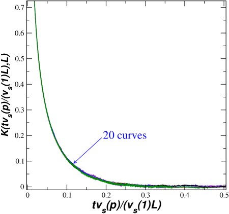
In Fig. 7 we show the data of Fig. 6 choosing for $v_{s}(p)/v_{s}(1)$ the values 1.538 ($p=0.1$), 1.300 ($p=0.5$), 0.703 ($p=1.5$) and 0.472 ($p=1.9$). Notice that the 20 sets of data collapse on a single curve.

Figure 7: The Family-Vicsek scaling function $K(tv_{s}(p),L)$ as a function of $tv_{s}(p)/v_{s}(1)L$ for $p=0.1,0.5,1.5,1.9$ and $L=1024,2048,4096,8192.$ The 20 sets of data collapse on a single curve.

In order to check that the determination of the sound velocity is correct, we have diagonalized the Hamiltonians up to $L=26$ sites for $p=0.5,1$ and 1.5 and looked at the second energy gap $E_{2}(p)$. The calculation of $E_{2}(p)$ is easier to calculate numerically as compared with $E_{1}$ since it corresponds to the smallest eigenvalue in the parity odd sector of the Hamiltonian. We have computed the ratios $E_{2}(0.5)/E_{2}(1)$ and $E_{2}(1.5)/E_{2}(1)$ which should converge for large $L$ to $v_{s}(0.5)/v_{s}(1)$ respectively $v_{s}(1.5)/v_{s}(1)$. Extrapolants give the values 1.307 respectively 0.6972 in excellent agreement with the values obtained from Family-Vicsek scaling.

We believe that in this way, we have shown that the PARPM belongs to the same universality class as the RPM for all values of $p$.

We give now an example which shows why it is useful to have models in the same universality class. Let us consider, in the stationary states, the average density of sites in which the slop vanishes (local minima and maxima):

$$\tau(L)=1/(L-1)\sum_{i=1}^{L-1}(1-|s_{i}|).$$ (3.8)

This quantity (ADSSV) was extensively used in the study of the phase diagram of the RPM [10]. There is a conjecture [11] about the values of $\tau(L)$ at the conformal invariant point of the RPM:

$$\tau(L)=(3L^{2}-2L+2)/(L-1)(4L+2).$$ (3.9)

This conjecture was checked on various lattice sizes. For large values of $L$, $\tau(L)$ has the following behavior:

$$\tau(L)=A+B/L+O(1/L^{2}),$$ (3.10)

where $A=3/4$ and $B=-1/8$. Are these coefficients universal? Using Monte Carlo simulations for lattices of different sizes (for $L$ up to 65000) we obtained the following results: $p=0.5,A=0.7500,B=0.219$; $p=1,A=0.7500,B=-0.125$; $p=1.99,A=0.7500,B=-0.302$.

We conclude that the average density of sites where the slope vanishes is a universal constant equal to 0.75 with the leading correction term being non-universal. An explanation of this interesting result in the context of conformal invariance is missing. It is also not clear if the ADSSV is a universal observable in other models defined on Dyck paths.

One can use the asymptotic value of $\tau(L)$ to have an estimate of the sound velocity. The average value of the density of peaks, equal to half the value of $\tau(L)$, is $<n_{c}>_{av}=3/8$. Substituting this value in (2.4), and using (2.7) one obtains

$$<q_{c}(p)>_{av}=\frac{v_{s}(p)}{v_{s}(1)}=\frac{8-3p}{5}.$$ (3.11)

Figure 8: Comparison of the ratios $v_{s}(p)/v_{s}(1)$ given by (3.11) (red line) and some of the estimated values (black dots) from the Family-Vicsek finite-size scaling.

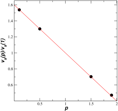
We have assumed that the fluctuations of the density of sites where the slop vanishes are small. One can compare the values obtained for $v_{s}(p)$ using (2.4) with those obtained from the diagonalization of the Hamiltonian and from Family-Vicsek scaling. In Fig. 8 we compare some of the results obtained from the Family-Vicsek scaling with the prediction in (3.11). The agreement is excellent. One notices that if $p$ approaches the value $p=2$, $v_{s}(p)/v_{s}(1)$ approaches the value 2/5. For the substrate the density of peaks is equal to 1/2, this gives, using (2.7) the value $v_{s}(2)=0$ for $p=2$. As a consequence, $v_{s}(p)$ decreases from the value 8/5 for $p=0$ to the value 2/5 if $p$ approaches the value 2 from below and has a discontinuity at $p=2$. At $p=2$ the substrate is an absorbing state.

4 Conclusions

The raise and peel model was up to now the single known conformal invariant growth model. The model described in this paper is different: it has rates which are dependent on global aspects of the configurations (the number of peaks). The fact that conformal invariance is maintained came as a surprise. The new model is not integrable and the stationary state does not have the remarkable properties of the RPM which are a consequence of integrability. Conformal invariance was tested for several values of the parameter $p$ by computing the density of contact points, the spectrum of the evolution operator and the Family-Vicsek scaling function. In the finite-size scaling limit, only the sound velocity depends on $p$.

Using the new model we have discovered that the average density of sites where the slope vanishes is, for large lattice sizes, a universal quantity and equal to 3/4 for any value of $p$. It would be interesting to look for other quantities which are universal. The model described here can be used as a tool to check universality.

As explained in the text, the parameter $p$ varies in the domain $0\leq p<2(L-1)/L$. For each value of $p<2$, one considers values of $L>2/(2-p)$ which makes sure that the rates are positive. We have observed that if $p$ approaches the value 2, the sound velocity decreases to a limiting value $v_{s}=2/5$, and one observes a slowing down in the time dependence of physical processes as one approaches the stationary state (see Figure 6).

An interesting phenomenon occurs if one chooses $p=2(L-1)/L$. Conformal invariance is lost and the stationary state is an absorbing state which is the substrate (see Figure. 1)). Although the stationary state is unique, for lattices sizes $L\mathchar 13350\relax 90$, the relaxation time is very long and increases exponentially with the size of the system. One observes metastable states. If the initial condition are changed, the system ends up in different metastable states. A detailed presentation of the $p=2(L-1)/L$ case will be published elsewhere [12].

5 Acknowledgments

We would like to thank J. Jaimes for discussions and to J. de Gier and P. Pearce for reading the manuscript and discussions. This work was supported in part by FAPESP and CNPq (Brazilian Agencies), by Deutsche Forschungsgemeinschaft (Germany) and by the Australian Research Council (Australia).

References

- [1] S. F. Edwards and D. R. Wilkinson, 1982 Proc. R. Soc. Lond. A 381 17
- [2] T. Halpin-Healy and Y.-C. Zhang, 1995 Phys. Rep. 254 215
- [3] J. de Gier, B. Nienhuis, P. Pearce and V. Rittenberg, 2003 J. Stat. Phys. 114, 1
- [4] F. C. Alcaraz, P. Pyatov and V. Rittenberg, 2007 J. Stat. Mech P07009
- [5] F. C. Alcaraz and V. Rittenberg, 2007 Phys. Rev. E 75 051110
- [6] F. C. Alcaraz and V. Rittenberg, 2010 J. Stat. Mech. bf P03024
- [7] A. V. Razumov and Yu. G. Stroganov, 2001 J. Phys. A 34 3185
- [8] M. T. Batchelor, J. de Gier and B. Nienhuis, 2001 J. Phys. A 34 L265
- [9] F. Family and E. Vicsek, 1985 J. Phys. A 18 L75
- [10] F. C. Alcaraz and V. Rittenberg, J. Stat. Mech. P07009 (2007)
- [11] Yu. G. Stroganov, private communication
- [12] F. C. Alcaraz and V. Rittenberg, to be published