Separation between coherent and turbulent fluctuations. What can we learn from the Empirical Mode Decomposition?

Nicolas Mazellier and Fabrice Foucher

Institut PRISME, 8, rue Léonard de Vinci, 45072 Orléans, FRANCE

Abstract

The performances of a new data processing technique, namely the Empirical Mode Decomposition, are evaluated on a fully developed turbulent velocity signal perturbed by a numerical forcing which mimics a long-period flapping. First, we introduce a "resemblance" criterion to discriminate between the polluted and the unpolluted modes extracted from the perturbed velocity signal by means of the Empirical Mode Decomposition algorithm. A rejection procedure, playing, somehow, the role of a high-pass filter, is then designed in order to infer the original velocity signal from the perturbed one. The quality of this recovering procedure is extensively evaluated in the case of a "mono-component" perturbation (sine wave) by varying both the amplitude and the frequency of the perturbation. An excellent agreement between the recovered and the reference velocity signals is found, even though some discrepancies are observed when the perturbation frequency overlaps the frequency range corresponding to the energy-containing eddies as emphasized by both the energy spectrum and the structure functions. Finally, our recovering procedure is successfully performed on a time-dependent perturbation (linear chirp) covering a broad range of frequencies.

1 Introduction

Most, if not all, engineering applications involving turbulent fluid flow undergo the influence of the so-called coherent structures. Even though their exact definition is still open to debate [1], their existence in turbulent flows is now commonly recognized since the beautiful flow visualization of a turbulent mixing layer by Brown and Roshko [2]. Their exact role in the onset of turbulence and their impact on the dynamics of turbulent interactions are of major interest in the development of relevant turbulence models. In particular, the strong persistence in space and time of such coherent structures may induce long-range memory implying, among others, a strong dependence of turbulence on boundary and initial conditions (see e.g. [3]). Evidence of such interplay were reported in recent experiments led, for instance, by Tong and Warhaft [4] on jet modification by means of a small ring located in the initial shear-layers, by Hu et al. [5] who investigated the effect of the corner radius onto the near-wake of a square cylinder or by Lavoie et al. [6] who studied the onset of turbulence generated by various shape of regular grid. Besides the fact that the flow topology is extremely sensitive to the modification of the initial conditions, the fundamental issue of their influence onto the energy transfer is still misunderstood [1]. This issue relates intimately to the concept of universality which is a key point in turbulence modeling.

Besides the fundamental issue of the interplay between coherent structures and turbulence, their management or control has attracted an increasingly interest in the scientific community in order to either favor or prevent their effects on a given process. For instance, the enhancement of mixing, required in processes such as non-premixed combustion, chemical reaction or wall cooling, can be achieved through the joint action of large-scale convection by coherent structures and the micro-mixing induced by turbulence. On the contrary, noise generation [4] and fluid-structure interaction phenomena, such as vortex-induced vibration experienced by freely movable bluff-body (see [7]), are extremely sensitive to the topology of coherent structures. Among the various strategies of flow control, the active closed-loop concept (referred to as reactive by Gad-el-Hak [8]) appears as the most attractive [9]. This approach is based on a feedback loop allowing for a real-time adaptation of the actuation in order to optimize a net energy gain. Unfortunately, unlike laminar flows, the straightforward implementation of this control strategy in turbulent flows is often disappointing and weakly efficient. The main drawback relies on the reliability of the reference signal used to drive to feedback loop control. Indeed, the pollution of this signal, which is basically expected to lock-in with the coherent structures, by the random fluctuations strongly alters the robustness of the control loop.

For all the above mentioned reasons, intense efforts have been dedicated to develop data analysis enabling to identify and extract the signature of the coherent structures from a turbulent signal. Hussain and Reynolds [10] introduced the so-called triple decomposition such that a physical variable of the turbulent flow, say the velocity for instance, results from the superimposition of three contributions: a coherent (i.e. phase-averaged), a mean (i.e. time average) and a random. Even though this definition allows for a clear separation between coherent structures and turbulent fluctuations, its application, in practice, is far to be easily tractable. Other attractive methods have been developed in order to organized motion in flows. One can cite, for instance, the Proper Orthogonal Decomposition (see e.g. [11] and references therein) which extracts modes sorted by their energy and is often used to define Reduced-Order Models (ROM) by keeping the first most energetic modes. Nevertheless, this approach provides a statistical description and therefore is subjected to convergence criteria which restrict its interest in the case of non-stationary dynamics. Inspired from the multi-scale feature of turbulence, wavelet analysis has brought significant insights in the understanding of the nonlinear interactions between the turbulent scales (see e.g. [12]). The main drawback of wavelet approach stands in the prescription of a given class of functions as the decomposition base.

In the nineties, Huang et al. [13] overcame these drawbacks by introducing the so-called Empirical Mode Decomposition (EMD). Basically, this data analysis technique decomposes a signal as the sum of a detail and a trend using its local envelopes. It is, therefore, entirely driven by the data themselves. In other words, the EMD does not require any a priori base function appearing, therefore, as an alternative way to investigate both non-stationary and non-linear physics. Although the EMD encountered a great success in various fields such as physics or biology, for instance, it has been introduced only very recently in the framework of turbulence. Huang et al. [14] investigated the intermittency of fully-developed turbulence by means of EMD and Hilbert transform. Foucher and Ravier [15] used the EMD in order to provide a triple-decomposition of turbulent signals forced by periodic or random excitation.

The work reported here is dedicated to the assessment of the performances of the EMD algorithm in discriminating between coherent signature and random fluctuation. For that purpose, the EMD is applied on a turbulent fluctuation perturbed by a numerical signal mimicking a long-period flapping. An original rejection procedure, based on a "resemblance" criterion, is proposed for discriminating between both contributions. The relevance of the EMD in separating the turbulent signal from the perturbation is evaluated in numerous conditions by varying both the amplitude and the frequency of the numerical flapping.

The paper is organized as follows. The basics of EMD analysis are given in Sec. 2. Then, the methodology used to separate the perturbation and the turbulent signal is described in Sec. 3. Especially, the "resemblance" criterion and the rejection procedure are introduced. Finally, the performances of the EMD is analyzed and discussed in Sec. 4.

2 The Empirical Mode Decomposition algorithm

In this section, the basics of EMD are briefly reminded and illustrated via a simple example. More details about the EMD method can be found in [13]. It is worth noticing that the EMD algorithm used in this study is computed by means of the Matlab scripts provided by Flandrin (http://perso.ens-lyon.fr/patrick.flandrin/).

2.1 The principles

The EMD method is based on the assumption that a signal $s(t)$ can be decomposed into the sum of a detail $d(t)$ and a trend $r(t)$, i.e.:

$$s(t)=d(t)+r(t).$$ (1)

The detail $d(t)$ is characterized by high frequency variations, whilst the trend $r(t)$ represents the low frequency variation. To illustrate this concept, let us consider the following "two-components" signal

$$s(t)=\sin{2\pi t}+\frac{1}{2}\sin{20\pi t}.$$ (2)

This signal is displayed in Fig. 1 which clearly evidences two time-scales. Rilling and Flandrin (2008) reported a complete investigation of the performances of EMD to analyze similar "two-components" signals. In particular, they evaluated the sensitivity of the EMD algorithm when varying separately the frequency ratio and the amplitude ratio between both contributions. It is worth noting that the specific example we use here belongs to the range delineated by Rilling and Flandrin (2008) where the EMD succeeds in separating the two tones.

Figure 1: Typical EMD analysis of a "two-components" signal $s(t)=\sin{2\pi t}+\frac{1}{2}\sin{20\pi t}$. (a) Evaluation of the local mean-value (thick solid line) as the average between the lower and the upper envelopes (dash lines). (b) Comparison of the estimated trend (solid line) and the low-frequency component $\sin{2\pi t}$ ($\circ$). (c) Comparison of the estimated detail (solid line) and the high-frequency component $\frac{1}{2}\sin{20\pi t}$ ($\circ$).

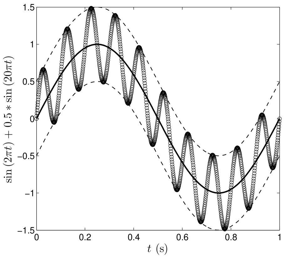
In order to extract the trend $r(t)$ from the signal, Huang et al. (1998) introduced the concept of the local mean value defined as the average between the lower ($e_{min}(t)$) and the upper ($e_{max}(t)$) envelopes of the signal, i.e.

$$r(t)=\frac{e_{min}(t)+e_{max}(t)}{2}.$$ (3)

To define these envelopes, Huang et al (1998) used a cubic interpolation between the local extrema of the signal. This is illustrated in Fig. 1 by the dashed lines, whilst the local mean value is represented by the solid line. Once the trend $r(t)$ has been evaluated, it is then easy to extract the detail $d(t)$ via Eq. (1).

The comparisons of the trend $r(t)$ and the detail $d(t)$, estimated from the signal $s(t)$ by means of the EMD algorithm, with the low- and high-frequency components (see Eq. (2)) are given in Figs. 1 and 1, respectively. The excellent agreement shown in these plots evidences the potentiality of the EMD.

2.2 The generalization

This procedure can be extended to any signal $s(t)$ containing more than two characteristic frequencies. In that case, the original signal $s(t)$ is first decomposed into two contributions according to Eq. (1). Then, the trend $r(t)$ resulting from this decomposition is used as a "new" signal onto which the EMD method is applied in turn. This procedure is reiterated until no more frequency can be identified. The original signal can therefore be expressed as follows

$$s(t)=\sum^{N}_{k=1}\mbox{IMF}_{k}(t)+r_{N}(t),$$ (4)

where $N$ is the total number of iterations, $r_{N}(t)$ is the final residue and $\mbox{IMF}_{k}(t)$ is the $k^{\mbox{th}}$ Intrinsic Mode Function, i.e. the trend of the $(k-1)^{\mbox{th}}$ iteration, extracted via the procedure described above. Given that the EMD is by definition a data-driven technique, therefore locally self-adaptive, two important remarks have to be made to emphasize the main differences between EMD and standard approaches:

1. the shape of the IMFs is not assumed a priori unlike the Fourier transform.

2. the extraction of the IMFs is not conditioned by a statistical convergence unlike the Proper Orthogonal Decomposition for instance.

These two degrees of freedom provide to the EMD method an attractive potential to study forced turbulence in the sense that the IMFs act as non-linear dynamic filters. This property is straightly related to the concept of instantaneous frequency. In order to define properly the instantaneous frequency, the IMFs have to fulfill two conditions (see [13]):

1. the total number of zero crossings and extremes differ by one at most.

2. the local mean value defined as the average between the lower and the upper envelopes is zero.

Huang et al. [13] developed a sifting procedure consisting in repeating, for each iteration, the EMD analysis until the IMF complies with both enumerated conditions. In the present study, we have restricted, for practical reason, the number of sifting repetition to 15 but no significant change has been observed when increasing this value.

3 The methodology

As mentioned earlier, the performances of the EMD algorithm are evaluated on an experimental turbulent signal which is artificially perturbed by a numerical long-period flapping. This section describes the strategy we have adopted to assess the relevance of the EMD to separate the perturbation from the reference signal.

Figure 2: EMD analysis of the reference signal $u_{i}(t)$ (a) and of a perturbed signal (b) with $f_{p}=10$Hz and $a_{p}=2$ m/s. In both cases, the top plot represents the analyzed signal.

3.1 The reference signal

The reference signal, used in this study, is a velocity fluctuation time-series measured in a fully-developed decaying turbulence. The experiment was carried out in an open-loop vertical wind tunnel of the laboratory CORIA (Rouen). The turbulence generator is a perforated plate with an uniform mesh size $M\approx 25mm$ set at the inlet of the working section. A detailed investigation of the turbulent flow produced downstream the perforated plate has been reported elsewhere by Mazellier et al. [16]. The streamwise velocity fluctuation sample $u_{i}(t)$ used here has been measured via Laser Doppler Velocimetry at approximately 15$M$ downstream the perforated plate where the flow is nearly homogeneous and isotropic (see [16] for more details). The main physical properties of the turbulent flow at this location are summarized in Table 1.

Table 1: Main physical characteristics of the reference turbulent flow

$U^{a}$ (m/s)	$\left<u_{i}^{2}\right>^{1/2}$ (m/s)	$L_{i}^{b}$ (mm)	$\lambda_{i}^{c}$ (mm)	$\eta_{i}^{d}$	$Re_{\lambda}^{e}$
4.1	0.57	9.4	1.6	0.1	59

^a Streamwise mean velocity,
^b Integral length-scale computed from Eq. (14),
^c Taylor microscale computed from Eq. (15),
^d Kolmogorov scale computed from Eq. (16),
^e Taylor-based Reynolds number ($\equiv\left<u_{i}^{2}\right>^{1/2}\lambda_{i}/\nu$ with $\nu$ the kinematic viscosity).

Note that the blockage ratio $\sigma$ of the perforated plate (defined as the ratio between the blocked area and the wind-tunnel’s section) used by Mazellier et al. [16] is significantly higher ($\sigma=0.67$) than that usually reported for bi-plane regular grids (see e.g. [17] with $\sigma=0.34$). This difference yields to a much higher turbulence intensity $\left<u_{i}^{2}\right>^{1/2}/U\approx 13$% (where $\left<\mbox{ }\right>$ denotes a time-averaging and $U$ the mean velocity) than that of standard grid-generated turbulence. However, regarding the dimension of the experiment, the turbulent flow is restricted to moderate Taylor-based Reynolds number $Re_{\lambda}$ ($\equiv\left<u_{i}^{2}\right>^{1/2}\lambda_{i}/\nu$ with $\nu$ the kinematic viscosity).

3.2 The perturbation

In this study, the general form of the numerical perturbation $p_{i}(t)$ is the following

$$p_{i}(t)=a_{p}(t)\sin\left(\phi(t)\right),$$ (5)

where $a_{p}$ and $\phi$ are the amplitude and the phase of the perturbation, respectively. The perturbation frequency $f_{p}$ and the phase are related by

$$\frac{d\phi}{dt}=2\pi f_{p}(t).$$ (6)

In the following, we report two cases mimicking either a "mono-component" or a "multi-component" flapping. The "mono-component" flapping is characterized by a constant perturbation frequency (sine wave), whilst $f_{p}$ is time-dependent, i.e. $f_{p}=f_{p}(t)$, for the case of the "multi-component" flapping (linear chirp).

The perturbed signal $u_{p}(t)$ under analysis is therefore

$$u_{p}(t)=u_{i}(t)+p_{i}(t).$$ (7)

The goal of the present work is to assess the ability of the EMD method to extract a long-period flapping from the turbulent signal. For that reason, the frequency range of the perturbation is much lower than the typical frequency $\left<u_{i}^{2}\right>^{1/2}/L_{i}$ of the integral length-scale ($\approx 60$Hz).

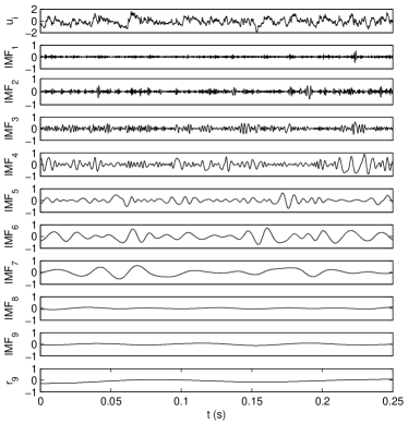
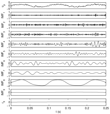
A typical EMD analysis of both the reference signal and a perturbed signal is displayed in Figs. 2 and 2, respectively. For that specific example, the amplitude $a_{p}$ and the frequency $f_{p}$ of the perturbation are equal to 2 m/s and 10 Hz, respectively. The presence of the perturbation is evident on the top plot of Fig. 2 where a long-period variation superimposes to the dynamics of the reference signal (see top plot of Fig. 2).

These plots suggest that the characteristic frequencies of the IMFs decrease with increasing IMF’s number meaning that the low frequency dynamics is mainly concentrated in the higher order IMFs. This statement is well supported by a close comparison of the IMFs time-series computed from both the reference and the perturbed signals. For that particular example, one can see that the IMFs are almost identical until $\mbox{IMF}_{6}$. For higher order IMFs, significant discrepancies can be observed, especially for $\mbox{IMF}_{8}$. A careful examination of that specific IMF with the perturbed signal (top plot in Fig. 2) reveals a strong resemblance in shape at low frequency.

3.3 The "resemblance" criterion

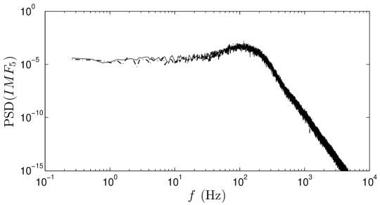
The simple example shown hereinbefore indicates that only a limited number of IMFs are polluted by the numerical perturbation. The issue arising from that observation relies on the relevant discrimination between "good", i.e. unpolluted, and "bad", i.e. polluted, IMFs. Foucher and Ravier [15] pointed out that this discrimination requires to define a criterion being robust and unbiased as well. In the case of the sum of two tones, Rilling and Flandrin [18] introduced a performance measurement based on the relative error of the reconstructed signal compared to the original one. Although this method shown a great efficiency, it requires to know a priori the reference signal which, obviously, is not available when studying real turbulent signals. Foucher and Ravier [15] recovered successfully the main large scale features of a turbulent flow exited by an external forcing by defining a tunable cut-off frequency. Their results revealed a strong dependence on that cut-off frequency enabling to determine an efficient value. Even though their approach gave good results, the assumption that the cut-off frequency is unique for each IMF is questionable. This is evidenced in Figs. 3-3 which show the Power Spectral Densities (PSD) of three IMFs extracted from both the reference signal and the perturbed signal exampled hereinbefore (see Figs. 2 and 2). As expected, the low-order IMF ($5^{\mbox{th}}$ IMF, here) is unaffected by the perturbation (see Fig. 3). One can see that the effect of the perturbation increases when increasing the IMF’s order. While the definition of a cut-off frequency may be appropriate in the case illustrated in Fig. 3 where a strong peak of energy appears at the excitation frequency, this strategy is irrelevant for the highest-order IMF shown in Fig. 3 due to the frequency shift accounted for the non-linear feature of the EMD algorithm.

Figure 3: 1D energy spectra of the (a) 5${}^{\mbox{th}}$ IMF, (b) 7${}^{\mbox{th}}$ IMF and (c) 9${}^{\mbox{th}}$ IMF time-series extracted from the reference signal (solid lines) and the perturbed signal (broken lines with dots) with $f_{p}=10$Hz and $a_{p}=2$m/s.

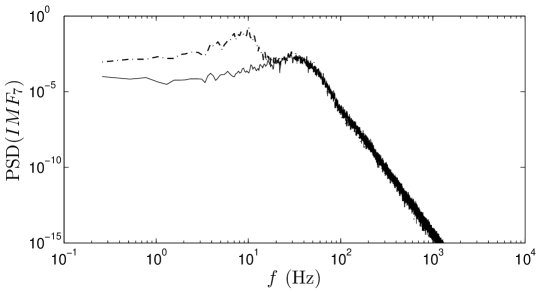
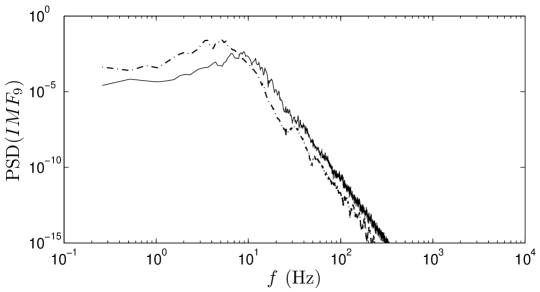
To address the issue of the separation between polluted and unpolluted IMFs, we introduce a new criterion, referred to as the "resemblance" criterion, $R(n)$ such that

$$\left\{\begin{array}[]{ll}R\left(n\right)=0&\mbox{ if }n=1,\\ &\\ R\left(n\right)=\frac{\left\langle u_{n}(t)u_{n-1}(t)\right\rangle}{\sqrt{\left\langle u_{n}(t)^{2}\right\rangle}\sqrt{\left\langle u_{n-1}(t)^{2}\right\rangle}}&\mbox{ if }1<n\leq N,\end{array}\right.$$ (8)

where the reconstructed signals $u_{n}(t)$ are defined as follows

$$\left\{\begin{array}[]{ll}u_{n}(t)=\sum^{n}_{k=1}\mbox{IMF}_{k}(t)&\mbox{ if }n<N,\\ &\\ u_{n}(t)=\sum^{n}_{k=1}\mbox{IMF}_{k}(t)+r_{N}&\mbox{ if }n=N,\end{array}\right.$$ (9)

with $n$ the reconstruction number. Eq. (9) represents the step-by-step reconstruction of the signal $u_{p}(t)$ by adding more and more IMFs. Therefore, the "resemblance" criterion $R(n)$ evaluates the statistical dependence between the reconstructed signals resulting from two successive steps. Fig. 4 shows the evolution of $R\left(n\right)$ in the specific case of the reference signal (i.e. unperturbed). Starting from 0 by definition, $R\left(n\right)$ increases monotonically with respect to $n$ until it saturates to 1 when $n$ tends towards $N$.

Figure 4: Evolution of the "resemblance" criterion $R(n)$ as a function of the reconstruction number $n$ for (a) the reference signal and perturbed signals: (b) $f_{p}=0.02$Hz, (c) $f_{p}=1$Hz and (d) $f_{p}=10$Hz. For each perturbed signal, the perturbation amplitude is constant ($a_{p}=2$m/s).

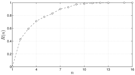
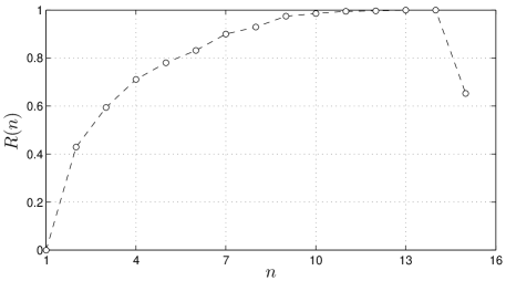
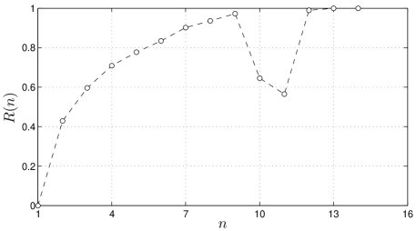
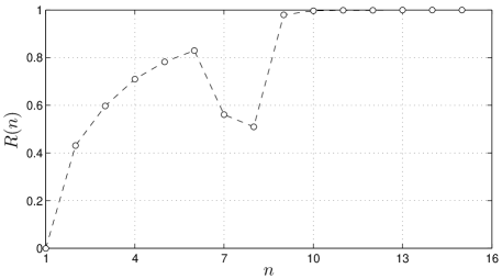
The efficiency of the "resemblance" criterion to discriminate between the perturbation and the reference signal relies on the fact that their dynamics (or more generally their physical properties) differs noticeably, in other words, their statistical dependence has to be small enough. This statement is emphasized in Figs. 4-4 which display the typical evolution of $R\left(n\right)$ for several perturbed signals. For these examples, the perturbation frequency $f_{p}$ is respectively $0.02$Hz, $1$Hz and $10$Hz, whilst the perturbation amplitude is kept constant ($a_{p}=2$ m/s). For each case, even though the global trend of $R(n)$ is similar to that obtained for the reference signal, a significant drop of $R\left(n\right)$ is easily detected. This fall results from the addition of a polluted IMF (i.e. a different dynamics) to the reconstructed signal which leads, therefore, to a decrease of the cross-correlation, i.e. the statistical dependence, between the $n^{\mbox{th}}$ and the $(n-1)^{\mbox{th}}$ reconstruction steps. Then, the "resemblance" criterion increases again reflecting the fact that the reconstructed signal becomes more and more resemblant to the perturbed signal. Note that for the specific case of $f_{p}=10$Hz, the drop of $R(n)$ coincides with the 7${}^{\mbox{th}}$ IMF in agreement with the spectral analysis displayed in Fig. 3.

3.4 The rejection procedure

Figs. 4-4 show that the reconstruction number $n$ where the fall of $R(n)$ occurs depends on $f_{p}$. This easily identifiable position is used to define a cut-off mode $k_{c}$ beyond which the IMFs are systematically discarded. It is important to remark that this procedure significantly differs from that used by Foucher and Ravier [15]. Indeed, the IMFs for which $k\geq k_{c}$ are all affected by the perturbation (see e.g. Fig. 3) and, therefore, are not used in the recovering procedure. This point is further discussed in Sec. 4.

Finally, we define the recovered signal $u_{r}(t)$ such as

$$u_{r}(t)=\sum^{k_{c}}_{k=1}\mbox{IMF}_{k}(t).$$ (10)

This signal can then be used to estimate, a posteriori, the perturbation

$$p_{r}(t)=u_{p}(t)-u_{r}(t),$$ (11)

with $p_{r}(t)$ the estimated perturbation. The recovered signal $u_{r}(t)$ can be assimilated to a "high-pass filtered" version of $u_{p}(t)$. Here, the term "high-pass filtering" has to be understood in a different way than usual. Indeed, as evidenced in Figs. 3-3, each IMF cover a broad range of frequency in the spectral space. In particular, a significant part of low-frequency energy (that of the turbulent large-scales) is contained in unpolluted IMFs. Consequently, unlike usual high-pass filtering, the recovering procedure does not annihilate totally the energy below a given cut-off frequency. This is illustrated in Sec. 4 where the performances of the recovering procedure is evaluated in various conditions.

4 Results

This section presents a qualitative and quantitative investigation assessing the EMD performances in discriminating the velocity signal from the perturbation. First, a parametric study, in the case of a "mono-component" perturbation (sine wave), is reported. Then, the influence of the perturbation frequency is analyzed, in details, by investigating the scale-by-scale turbulent energy by means of energy spectra and structure functions. A particular attention is given to the main turbulence properties at large- and small-scales. Finally, the results of the extension to a time-dependent perturbation (linear chirp) are provided.

4.1 The "mono-component" flapping

An extensive investigation of the influence of both parameters $a_{p}$ and $f_{p}$ has been conducted following the procedure described in Fig. 5 in the case of a "mono-component" perturbation. At each iteration of this parametric study, a couple ($a_{p}$, $f_{p}$) is fixed and the recovering algorithm described in Sec. 3 is applied on the perturbed signal in order to extract, a posteriori, the velocity signal and the perturbation according to Eqs. (10) and (11). In this study, the ratio of the perturbation energy ($a_{p}^{2}/2$) to the turbulent kinetic energy ($\left<u_{i}^{2}\right>$) is lower than 25. Furthermore, in order to simulate a long-period flapping, the maximum perturbation frequency $f_{p}$ is about 6 times smaller than the frequency of the energy-contained eddies ($\equiv\left<u_{i}^{2}\right>^{1/2}/L_{i}$).

Figure 5: Schematic of the procedure followed to recover $u_{r}(t)$ and $p_{r}(t)$ from the perturbed signal $u_{p}(t)$.

The quality of the recovering algorithm can be assessed by means of the coefficient $C$ defined as follows

$$C=\frac{\left\langle u_{i}(t)u_{r}(t)\right\rangle}{\sqrt{\left\langle u_{i}^{2}\right\rangle}\sqrt{\left\langle u_{r}^{2}\right\rangle}}.$$ (12)

The variation of $C$ as a function of the couple ($a_{p},f_{p}$) is plotted in Figs. 6 and 6 for a signal duration $t_{m}$ of about 2s ($2^{15}$ samples) and 15s ($2^{18}$ samples), respectively.

Figure 6: Contour plot of the recovering quality indicator $C$ with respect to the parameters of the "mono-component" perturbation. Length of the reference signal: (a) $t_{m}\approx$ 2s ($2^{15}$ samples), (b) $t_{m}\approx$ 15s ($2^{18}$ samples).

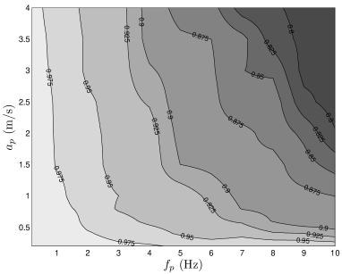
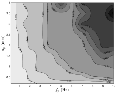
The high values of $C$ (mostly $\geq 0.8$) observed in both plots reflect that the recovering procedure based on the EMD algorithm performs remarkably well over the whole range of perturbation amplitude and frequency tested. Excluding the area where $a_{p}\geq 3$, a close comparison between both plots indicates that the influence of the signal length on the recovering quality is weak. Therefore, in the following, only results obtained for $t_{m}\approx$ 15s ($2^{18}$ samples) are reported.

Overall, the recovering procedure seems less sensitive to $a_{p}$ than to $f_{p}$ and it turns out that the quality of the recovering procedure decreases with increasing $f_{p}$. In order to analyze this feature, we now focus the discussion, on three typical "mono-component" perturbations differing only by their frequency, i.e. $f_{p}=0.02$Hz, 1Hz and 10Hz respectively, while their amplitude is kept constant ($a_{p}=2$m/s). These specific frequencies cover the entire range of flapping frequency simulated in this study.

Figure 7: Recovered signals $u_{r}(t)$ (dashed lines) vs reference signal $u_{i}(t)$ (solid lines) for three perturbation frequencies ($a_{p}=2$ m/s): (a) $f_{p}=0.02$Hz, (d) $f_{p}=1$Hz and (g) $f_{p}=10$Hz. Comparison between the original perturbations $p(t)$ and the a posteriori estimated perturbation $p_{r}(t)$ for three perturbation frequencies ($a_{p}=2$ m/s): (b) $f_{p}=0.02$Hz, (e) $f_{p}=1$Hz and (h) $f_{p}=10$Hz. Joint-PDF between the recovered signal $u_{r}(t)$ and the reference signal $u_{i}(t)$ for three specific "mono-component" perturbations: (a) $f_{p}=0.02$Hz, (b) $f_{p}=1$Hz and (c) $f_{p}=10$Hz. For each case, the perturbation amplitude is kept constant $a_{p}=2$m/s.

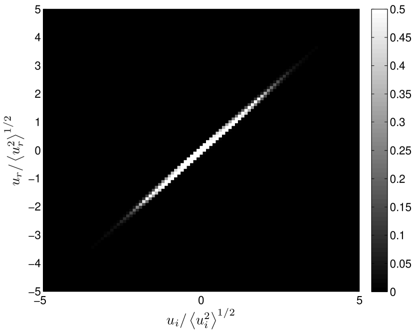
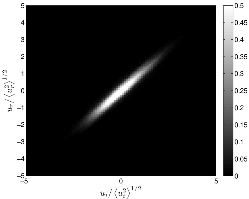
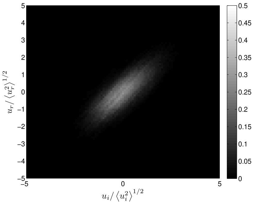
The comparison between the recovered velocity signals $u_{r}(t)$ and the reference velocity signal $u_{i}(t)$ is given in Figs. 7, 7 and 7 for $f_{p}=0.02$Hz, 1Hz and 10Hz, respectively. For the smallest perturbation frequency, i.e. $f_{p}=0.02$Hz, an impressive agreement between $u_{r}(t)$ and $u_{i}(t)$ is found. This is emphasized by the joint-PDF between both signals plotted in Fig. 7 which testifies that $u_{r}(t)$ and $u_{i}(t)$ are almost indistinguishable. Furthermore, we draw the reader’s attention to the excellent collapse of the a posteriori estimated perturbation $p_{r}(t)$ on the original perturbation $p_{i}(t)$, as shown in Fig. 7, even though the signal duration is much smaller than one period of the perturbation. It is worth noticing that standard approaches, such as Fourier transform for instance, would have failed in such accurate deduction because at least one period of the perturbation would have been needed. This is an important feature of the EMD algorithm in order to study unsteady and non-linear dynamics, in the sense it is a data-driven feature, i.e. without prescribing, a priori, the base functions.

For higher perturbation frequencies, $u_{r}(t)$ compares fairly well with $u_{i}(t)$, although slight departures are visible (see Figs. 7 and 7). These discrepancies increase with increasing $f_{p}$, as evidenced by the joint-PDF displayed in Figs. 7 and 7 for $f_{p}$=1Hz and 10Hz, respectively. Nevertheless, a careful examination of the worst case, i.e. $f_{p}=10$Hz, reveals that the fast dynamics (high frequency) of the velocity signal is successfully inferred from the perturbed signal. Therefore, the main observable differences between $u_{r}(t)$ and $u_{i}(t)$ pertain to their low frequency part. This is emphasized by the comparison between the a posteriori estimated perturbation $p_{r}(t)$ and the original perturbation $p_{i}(t)$ shown in Figs. 7 and 7.

4.2 The scale-by-scale turbulent energy

A deeper analysis of the recovering procedure can be performed by comparing the 1D energy spectra $E_{\theta}$ (defined as $\left<u_{\theta}^{2}\right>=\int_{0}^{\infty}E_{\theta}(f)df$, with $f$ the spectral frequency), where the subscript $\theta$ refers to either the reference, the perturbed or the recovered velocity signal. Such a comparison is given in Figs. 8, 8 and 8 for the perturbation frequency $f_{p}=0.02$Hz, 1Hz and 10Hz, respectively. In each case, the perturbation appears as a sharp peak centered on the frequency $f_{p}$, even though, as mentioned earlier, for the lowest perturbation frequency one cannot inferred a posteriori the value of $f_{p}$ from the spectral analysis.

Figure 8: 1D energy spectra of the reference signal $u_{i}(t)$ (solid line), perturbed signals $u_{p}(t)$ (dotted lines) and recovered signals $u_{r}(t)$ (dashed lines) for three perturbation frequencies ($a_{p}=2$ m/s): (c) $f_{p}=0.02$Hz, (f) $f_{p}=1$Hz and (i) $f_{p}=10$Hz.

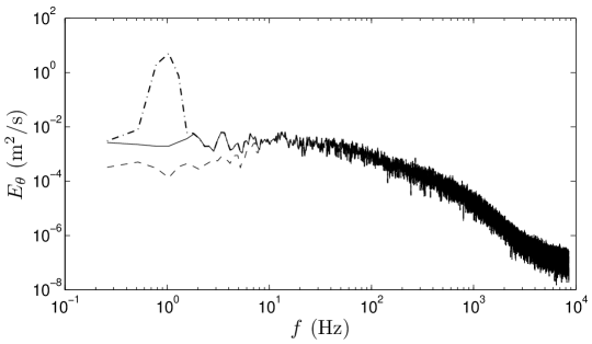
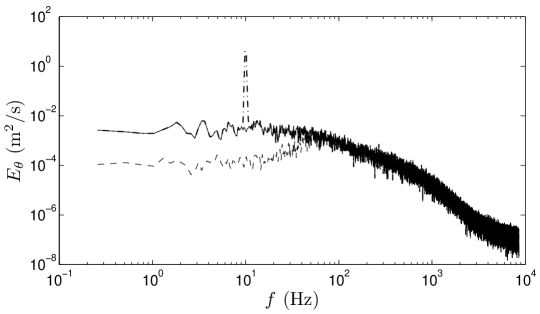
One can easily see that both the intermediate inertial range and the high frequencies of the energy spectra computed from $u_{r}(t)$ are mostly unaffected by the recovering procedure, independently of the perturbation frequency. This result proves that the fast dynamics of the reference signals is extracted with success from the perturbed velocity signals. The major discrepancies between $E_{r}(f)$ and $E_{i}(f)$ occur in the range $f\leq f_{p}$. One can see that the characteristic plateau at low frequency exhibited by $E_{i}(f)$ [19] is underestimated by the recovering procedure. Both the energy loss and the range of affected frequencies $f$ increase with increasing $f_{p}$. This feature relies on the way our filtering procedure is designed to reject the high-order polluted IMFs according to the "resemblance" criterion, as described in Sec. 2. Indeed, the energy of the rejected IMFs is mostly concentrated at low frequency (see e.g. Figs. 3-3).

It is not clear whether the intrinsic features of the EMD algorithm, alone, account for this drawback. Schlotthauer et al. [20] documented an extensive study of the influence of parameters such as signal length and sifting number. They found out that the statistical properties of the IMFs of a gaussian white noise strongly depend on these parameters. Another way which can explain this phenomenon stands in the concept of the local mean value which is defined as the local average of the signal envelopes. A careful examination reveals that these envelopes can locally either overshoot or truncate the analyzed signal, altering, therefore, the quality of the EMD algorithm. Besides these numerical aspects, one may expect that physical reasons can also account for the deterioration of the recovering quality with increasing $f_{p}$. Indeed, when the perturbation frequency overlaps the energy-containing frequency range (i.e. the large-scales), one may expect their respective dynamics to mix, leading to a less efficient separation by means of the EMD algorithm. Rilling and Flandrin [18] reported that both modes of a "two-components" signal can be sometimes unfruitfully separated by the EMD method, depending on the frequency ratio of both modes as well as their relative amplitude.

Nevertheless, it is worth noting that even though a significant part of the energy at low frequency is lost during the rejection procedure, this is much less severe than standard high-pass filtering. Furthermore, one can argue that band-pass filtering could have performed more efficiently but such approach implies the unwanted frequency band to be clearly identifiable. This point is of particular importance, especially for the case of "multi-component" perturbation which is investigated at the end of this section.

As pointed out by Huang et al. [13], the use of the Fourier transform (and related tools) to study non-stationary physics is meaningless. The scale-by-scale investigation of the turbulence by means of the structure functions is an alternative and complementary way to the spectral analysis. Structure functions are defined as the statistical moments of the velocity increments, i.e. the velocity difference between two points separated by a time increment $\tau$ [21], which, in this study, are restricted to the streamwise velocity increment

$$\delta u_{\theta}(\tau)=u_{\theta}(t+\tau)-u_{\theta}(t).$$ (13)

The dimensionless second-order structure function $\left<(\delta u_{\theta})^{2}\right>/\left<u_{i}^{2}\right>$ computed from the reference, perturbed and recovered velocity signals are plotted in Figs. 9, 9 and 9 for $f_{p}=$0.02Hz, 1Hz and 10Hz, respectively.

Figure 9: Second-order structure functions of the reference ($\circ$), perturbed ($\triangledown$) and recovered ($\star$) velocity signals for (a) $f_{p}=0.02$Hz, (b) $f_{p}=1$Hz and (c) $f_{p}=10$Hz. For each perturbed signal, the perturbation amplitude is constant ($a_{p}=2$m/s). The scaling law $\tau^{2/3}$ is represented by the dash lines.

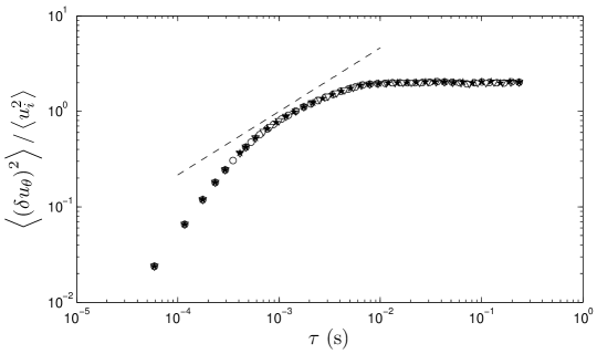
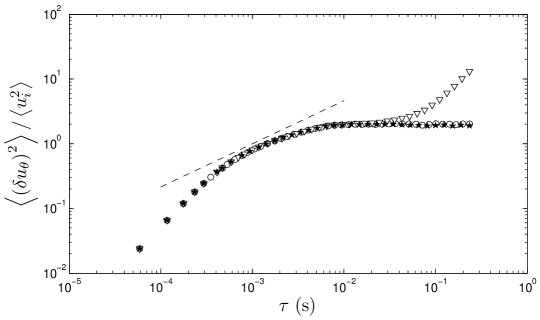
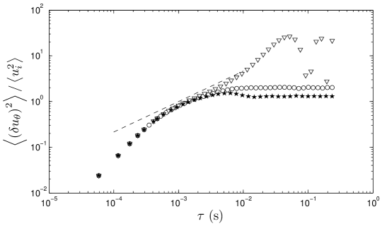
Physically, $\left<(\delta u_{\theta})^{2}\right>$ represents the energy of a scale $\ell$, where the spatial separation is deduced from the time lag $\tau$ by means of the Taylor’s hypothesis, i.e. $\ell=-U\tau$. One can show that $<\left(\delta u_{\theta}\right)^{2}>$ tends towards $2\left<u_{\theta}^{2}\right>$ for large time (or space according to the Taylor’s hypothesis) separation, i.e. when $\tau\rightarrow\infty$. This expectation is well supported by the results computed from the reference velocity signal. Moreover, a narrow inertial range can be identified by the scaling law $\left<(\delta u_{\theta})^{2}\right>\propto\tau^{2/3}$, equivalent to the well-known $-5/3$ scaling law in spectral space [22, 19].

Obviously, the long-period flapping, simulated by the numerical perturbation, has a significant effect at large $\tau$, especially for the two highest perturbation frequencies (see Figs. 9 and 9). Furthermore, in the case of $f_{p}=10$Hz, the perturbation affects also the beginning of the inertial range.

The results obtained for the recovered velocity signals clearly evidence the high quality of the recovering procedure, in particular for $f_{p}=0.02$Hz and 1Hz. In both cases, an impressive collapse onto the reference second-order structure function is found. These results indicate that, for $f_{p}=0.02$Hz and 1Hz, the amount of turbulent energy contained in the rejected IMFs is almost negligible in comparison with the turbulent kinetic energy $\left<u_{i}^{2}\right>$. For the highest frequency perturbation, i.e. $f_{p}=$10Hz, although the plateau value is underestimated after the recovering procedure (notice that less than half of the IMFs are kept according to Fig. 4), the influence of the perturbation is successfully annihilated, particularly regarding the inertial range.

4.3 The turbulence properties

The quantitative assessment of the recovering quality can be done by comparing the statistical properties of both the reference and the recovered velocity signals, at large- and small-scales. The large-scales are featured by both their energy, i.e. $\left<u_{\theta}^{2}\right>$, and the integral length-scale

$$L_{\theta}=\frac{U}{u_{\theta}^{\prime 2}}\int_{0}^{\infty}\left\langle u_{\theta}(t)u_{\theta}(t+\tau)\right\rangle d\tau.$$ (14)

The small-scales can be described through the Taylor micro-scale

$$\lambda_{\theta}=U\sqrt{\frac{\left<u_{\theta}^{2}\right>}{\left<\left(\frac{\partial u_{\theta}}{\partial t}\right)^{2}\right>}},$$ (15)

and the Kolmogorov scale

$$\eta_{\theta}=\left(\frac{\nu^{3}}{\epsilon_{\theta}}\right)^{1/4},$$ (16)

where $\epsilon_{\theta}$ ($\equiv\frac{15\nu}{U^{2}}\left\langle\left(\frac{\partial u_{\theta}}{\partial t}\right)^{2}\right\rangle$ under isotropic assumption) is the turbulent kinetic energy dissipation rate.

The ratios $(\left<u_{r}^{2}\right>/\left<u_{i}^{2}\right>)^{1/2}$, $\lambda_{r}/\lambda_{i}$ and $L_{r}/L_{i}$ are plotted in Fig. 10 with respect to $f_{p}$. One can see that the differences between the recovered and the reference signals increase with increasing $f_{p}$. The staircase-like shape of the curves is related to the rejection method which acts as a discrete filter. Each step corresponds to the rejection of an additional IMF.

Over the whole range of $f_{p}$ tested here, the recovering of $\left<u_{r}^{2}\right>^{1/2}$ is better than 80%. Furthermore, we have shown, hereinbefore, that the high frequency dynamics is unaffected by the recovering algorithm implying, therefore, that the statistics of the derivatives are almost unchanged, i.e. $\epsilon_{r}\approx\epsilon_{i}$ and $\eta_{r}\approx\eta_{i}$. Consequently, according to Eq. (15), the uncertainties in the evaluation of $\lambda_{r}$ relies only on those of $\left<u_{r}^{2}\right>^{1/2}$, explaining why $(\left<u_{r}^{2}\right>/\left<u_{i}^{2}\right>)^{1/2}$ and $\lambda_{r}/\lambda_{i}$ are almost indistinguishable.

Figure 10: Variation of $(\left<u_{r}^{2}\right>/\left<u_{i}^{2}\right>)^{1/2}$ ($\square$), $\lambda_{r}/\lambda_{i}$ ($+$) and $L_{r}/L_{i}$ ($\circ$) against $f_{p}$.

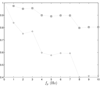
The largest discrepancies are observed for the integral length-scale which is significantly underestimated, by about 60% for the highest $f_{p}$. This result can be explained by reformulating Eq. (14) under the following form [19]

$$L_{\theta}=\frac{UE_{\theta}(f=0)}{4\left<u_{\theta}^{2}\right>}.$$ (17)

As shown previously (see e.g. Fig. 8), the term $E_{r}(f=0)$ is dramatically affected by the rejection procedure, even though it would have been worst with a classical high-pass filter. The strong decrease in $E_{r}(f=0)$ accounts for the underestimation of $L_{r}$. This is an important difference with $\left<u_{r}^{2}\right>$ which is computed from the integration of $E_{r}$ and is, therefore, less affected by the energy loss at low frequency.

An important issue, linked to the interaction between large- and small scales, arises from these results. Investigating the features of the zero-crossing of the velocity fluctuation in various experiments, [23] found out an universal relationship between the dissipation constant and the large-scale flow topology. Consequently, one may assume that the alteration of the large-scale properties (highlighted by the underestimation of the integral length-scale) might also modify directly or not the inertial range and/or the small-scale properties. This issue might actually be addressed through the investigation of the third-order structure function $\left<(\delta u_{\theta})^{3}\right>$ which represents the energy transfer at a given scale. In the following, for sake of simplicity, we consider the spatial separation $\ell$ instead of the time separation $\tau$. For high enough Reynolds number, the dimensionless third-order structure function $S_{3\theta}=-\left<(\delta u_{\theta})^{3}\right>/(\epsilon_{\theta}\ell)$ is expected to reach a constant value in the inertial range [21]

$$S_{3\theta}=\frac{4}{5}.$$ (18)

Using independent approaches, Qian [24] and afterwards Lundgren [25] proposed corrections of Eq. (18) accounting for the effects of the finite Reynolds number in the framework of freely decaying turbulence. These corrections can be expressed under the following form

$$S_{3\theta}=\frac{4}{5}-C_{1}\left(\frac{\ell}{\ell_{o}}\right)^{\alpha}-C_{2}\left(\frac{\ell}{\ell_{i}}\right)^{\beta},$$ (19)

where $\ell_{o}$ and $\ell_{i}$ represent an outer scale (i.e. large scale) and an inner scale (i.e. viscous scale), respectively. For decaying turbulence, the exponents $\alpha$, $\beta$ and the numerical constants $C_{1}$, $C_{2}$ are equal to $2/3$, $-4/3$ and $3.34/\sqrt{15}$, $8$, respectively (see Eq. (4) given by Gagne et al. [26]). This relationship accounts for the influence of the large- and small-scales on the energy transfer at a scale $\ell$. Taking $\ell_{o}=L_{\theta}$ and $\ell_{i}=\eta_{\theta}$, the maximum value reached by $S_{3\theta}$ (defined by $dS_{3\theta}/d\ell=0$), according to Eq. (19), is

$$S_{3\theta}^{max}=\frac{4}{5}-\gamma\left(\frac{\eta_{\theta}}{L_{\theta}}\right)^{4/9},$$ (20)

with $\gamma=3/2C_{1}(2C_{2}/C_{1})^{1/3}\approx 3.42$. Gagne et al. [26] reported a good agreement between this prediction and experimental data obtained in various turbulent flows. These authors proposed a Reynolds-correction to compensate for the deviation at large- and small-scale. Even though the data collapsing was significantly improved, the use of these corrections is beyond the scope of the present study where we essentially focused on the maximum value of $S_{3\theta}$. Indeed, one of the main interests of Eq. (20) is to provide an alternative way to Eq. (14) to estimate $L_{\theta}$.

Figure 11: Evolution of $S_{3i}$ ($\circ$) and $S_{3r}$ ($\star$) with respect to $\ell$ (inferred from the time separation $\tau$ by means of the Taylor’s hypothesis). The solid line symbolizes the "$4/5$" law [21]. The dashed line symbolizes the Lundgren’s prediction [25] for the reference signal according to Eq. (20). These results have been obtained for a "mono-component" perturbation with $f_{p}=10$Hz and $a_{p}=2$m/s.

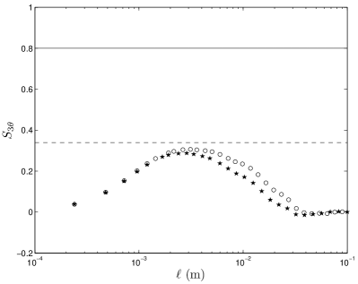
The evolution of $S_{3\theta}$ computed from $u_{i}(t)$ and $u_{r}(t)$ is plotted in Fig. 11 against $\ell$. It is worth noting that no significant difference between $S_{3i}$ and $S_{3r}$ has been observed for $f_{p}=0.02$Hz and 1Hz. Therefore, only the results obtained for the worst case, i.e. $f_{p}=10$Hz are reported in Fig. 11. The maximum value of $S_{3i}$ according to Eq. (20) is displayed in this plot. To emphasize the relevance of the Lundgren’s corrections, the "4/5" law is also plotted. One can clearly see that the Lundgren’s prediction is a good approximation of $S_{3i}^{max}$, even though the theoretical inertial range plateau is slightly overestimated. The discrepancies between the expected and the experimental values of $S_{3i}^{max}$ may be accounted for the non-stationarity feature of decaying turbulence as pointed out by Danaila et al. [27].

The comparison between $S_{3i}$ and $S_{3r}$ shows that the influence of the recovering procedure is noticeable at large-scale and in the inertial range as well. The decrease of the Reynolds number $Re_{\lambda}$, due to the underestimation of both the turbulent kinetic energy and the Taylor micro-scale, may account for these results (see e.g. Fig. 1 of [26]). Thanks to the measurement of $S_{3\theta}^{max}$, the integral length-scale of the recovered signal, $L_{r}$, can be estimated according to Eq. (20). In that case, the ratio $L_{r}/L_{i}$ is found to be better than 90%. This is an impressive improvement compared to the values reported in Fig. 10. It seems, therefore, that even though the rejection method can alter the statistical properties of the turbulent signal, the underlying physics is still conserved during the recovering procedure. This may be accounted for the specific features of the IMFs which span a broad band of frequencies (or wavenumbers) as evidenced in Figs. 3-3. These plots support the idea that each IMF contains a more or less important part of large- and small-scale information.

4.4 The non-stationary flapping

We close this section by assessing the performances of the recovering procedure on a time-dependent perturbation mimicking the non-stationary feature often encountered in engineering applications (e.g. unsteady injection in engines). For that purpose, the perturbation added to the reference signal is a linear chirp, i.e. $f_{p}(t)=f_{0}(t/t_{m})$ with $f_{0}=10$Hz ($a_{p}=2$m/s). The perturbation frequency sweeps the entire range previously reported for the "mono-component" perturbation.

The recovered velocity signal $u_{r}$ and the a posteriori estimated perturbation $p_{r}$ are compared with their reference counterparts in Figs. 12 and 12, respectively.

Figure 12: (a) Recovered velocity signal $u_{r}$ (dash line) compared with the reference velocity signal $u_{i}$ (solid line). (b) A posteriori estimated perturbation $p_{r}$ (dash line) compared with the original perturbation $p_{i}$ (solid line). These results have been obtained in the case of the time-dependent perturbation (linear chirp).

The excellent agreement between the recovered and the original signals testifies to the efficiency of the EMD algorithm in separating both contributions. This claim applies especially regarding the dynamics of both the velocity and the perturbation, albeit in the frequency range investigated in this study. Even though a weak scatter is noticeable at low perturbation frequency (see Fig. 12), the rejection procedure captures successfully the frequency shift and the perturbation amplitude as well.

Figure 13: (a) 1D energy spectra computed from $u_{i}$ (solid line), $u_{p}$ (broken line with dots) and $u_{r}$ (dash line). (b) Dimensionless third-order structure function computed from $u_{i}$ ($\circ$) and $u_{r}$ ($\star$) against the separation scale $\ell$ (inferred via the Taylor’s hypothesis). These results have been obtained in the case of the time-dependent perturbation (linear chirp).

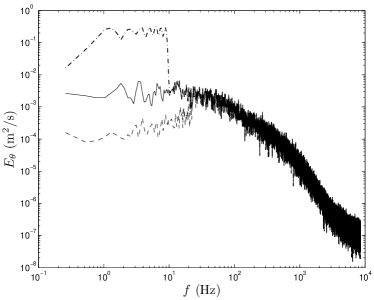
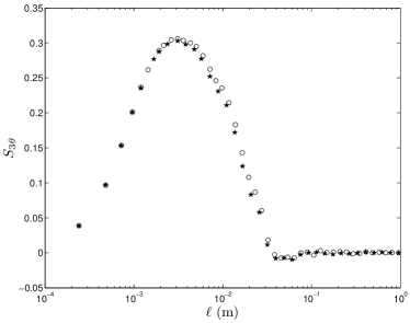
The effect of the rejection procedure is highlighted by the energy spectra plotted in Fig. 13. As expected, the perturbation (linear chirp) adds a large amount of energy over a broad range of frequency. One can clearly see that the recovering algorithm annihilates the energy contained in the numerical perturbation, even though the turbulent energy $E_{r}$ is underestimated in the low frequency range as observed in the case of the "mono-component" perturbation. However, the energy transfer through scales is much less altered by the rejection process as shown by the dimensionless third-order structure function $S_{3\theta}$ displayed in Fig. 13. This can be partly explained by the fact that the highest frequencies of the perturbation are less energetic than in the investigation of the "mono-component" perturbation.

5 Conclusion

The performances of a new data analysis method, namely the Empirical Mode Decomposition, have been assessed on a perturbed turbulent velocity signal. A numerical perturbation, whose parameters (amplitude and frequency) can vary in time, has been added to the reference signal in order to mimic a long-period flapping, i.e. the perturbation frequency remains lower than the typical frequency featuring the energy-contained eddies of the turbulent flow. The EMD algorithm has been used to recover, a posteriori, both the reference signal and the perturbation. For that purpose, a rejection procedure, acting such as a high-pass filter, has been designed. This procedure is based on the "resemblance" criterion, introduced for the first time in this paper, enabling to discriminate between the perturbed and the unperturbed modes deduced from the EMD.

First, an extensive investigation of the EMD efficiency has been performed and discussed in the case of a "mono-component" perturbation (sine wave) varying both its amplitude and its frequency. It has been shown that the EMD performances are mainly affected by the frequency parameter. This result has been emphasized by the analysis of both the energy spectrum and the second-order structure function revealing that the recovering procedure is significantly altered when the perturbation frequency overlaps the frequency range of the energy-containing eddies. Although the turbulent energy loss at large-scale, due to the high-pass filtering scheme, the dynamics of both the inertial and the dissipative ranges are successfully reproduced. Especially, we have pointed out that the energy transfer through scales is satisfactorily recovered by studying the third-order structure functions. Then, the relevance of the EMD algorithm has been addressed in the specific case of a non-stationary perturbation (linear chirp). Our results have shown that the recovering procedure developed in this study performs with great success over the broad range swept by the perturbation frequency.

This study highlights the potential of the EMD algorithm in the study of turbulence and its interplay with coherent structures. These encouraging results rely on the ability to extract a local trend, i.e. the local mean-value, in a fluctuating signal which is of great interest in the framework of closed-loop flow control.

References

- [1] A. K. M. F. Hussain. Coherent structures - reality and myth. Phys Fluids, 26(10):2816–2850, 1983.
- [2] G. L. Brown and A. Roshko. On density effects and large structure in turbulent mixing layer. J Fluid Mech, 54:775–816, 1974.
- [3] W K George. The decay of homogeneous turbulence. Phys Fluids A, 4:1492, 1992.
- [4] C Tong and Z Warhaft. Turbulence suppression in a jet by means of a fine ring. Phys Fluids, 6:328, 1994.
- [5] J C Hu, Y Zhou, and C Dalton. Effects of the corner radius on the near wake of a square prism. Exp Fluids, 40:106–118, 2006.
- [6] P Lavoie, P Burratini, L Djenidi, and R A Antonia. Effect of initial conditions on decaying grid turbulence at low . Exp Fluids, 39:865, 2005.
- [7] P W Bearman. Vortex shedding from oscillating bluff bodies. Annual Review of Fluid Mechanics, 16:195–222, 1984.
- [8] M Gad-el Hak. Flow Control: Passive, Active and Reactive Flow Management. Cambridge University Press, London, 2000.
- [9] Haecheon Choi, Woo-Pyung Jeon, and Jinsung Kim. Control of flow over a bluff body. Annual Review of Fluid Mechanics, 40(1):113–139, 2008.
- [10] A. K. M. F. Hussain and W. C. Reynolds. The mechanics of an organized wave in turbulent shear flow. J Fluid Mech, 41:241–258, 1970.
- [11] G Berkooz, P Holmes, and J L Lumley. The proper orthogonal decomposition in the analysis of turbulent flows. Annual Review of Fluid Mechanics, 25:539–575, 1993.
- [12] Marie Farge, Giulio Pellegrino, and Kai Schneider. Coherent vortex extraction in 3D turbulent flows using orthogonal wavelets. Phys. Rev. Lett., 87(5), 2001.
- [13] N. E. Huang, Z. Shen, S. R. Long, W. C. Wu, H. H. Shih, Q. Zheng, N. C. Yen, C. C. Tung, and H. H. Liu. The empirical mode decomposition and the hilbert spectrum for nonlinear and non-stationary time series analysis. Proc. R. Soc. Lond. A, 454:903–995, 1998.
- [14] Y. X. Huang, F. G. Schmitt, Z. M. Lu, and Liu Y. L. An amplitude-frequency study of turbulent scaling intermittency using empirical mode decomposition and hilbert spectral analysis. Europhys Lett, 84:40010, 2008.
- [15] F Foucher and P Ravier. Determination of turbulence properties by using empirical mode decomposition on periodic and random perturbed flows. Exp Fluids, 49:379–390, 2010.
- [16] N. Mazellier, L. Danaila, and B. Renou. Multi-scale turbulence injector: a new tool to generate intense homogeneous and isotropic turbulence for premixed combustion. J Turb, 11(43):1–30, 2010.
- [17] G. Comte-Bellot and S. Corrsin. The use of a contraction to improve isotropy of grid-generated turbulence. J Fluid Mech, 25:657–682, 1966.
- [18] G. Rilling and P. Flandrin. One or two frequencies? the empirical mode decomposition answers. IEEE Trans on Signal Proc, 56:85–95, 2008.
- [19] S. B. Pope. Turbulent flows. Cambridge University Press, New-York, 2000.
- [20] G. Schlotthauer, M. E. Torres, H. L. Rufiner, and P. Flandrin. EMD of gaussian white noise: effects of signal length and sifting number on the statistical properties of intrinsic mode functions. Adv Adapt Data Analys, 1(4):517–527, 2009.
- [21] U Frisch. Turbulence: the legacy of A.N. Kolmogorov. Cambridge University Press, New-York, 1995.
- [22] H. Tennekes and J. L. Lumley. A first course in turbulence. MIT Press, Cambridge, 1972.
- [23] N. Mazellier and J. C. Vassilicos. The dissipation constant is not universal because of its universal dependence on large-scale flow topology. Phys Fluids, 20, 2008.
- [24] J. Qian. Slow decay of the finite reynolds number effect of turbulence. Phys Rev E, 60(3):3409–3412, 1999.
- [25] T. S. Lundgren. Kolmogorov two-thirds law by matched asymptotic expansion. Phys Fluids, 14(2):638–642, 2002.
- [26] Y Gagne, B Castaing, C Baudet, and Y Malécot. Reynolds dependence of third-order velocity structure functions. Phys Fluids, 16(2):482–485, 2004.
- [27] L. Danaila, F. Anselmet, T. Zhou, and R. A. Antonia. A generalization of Yaglom’s equation which accounts for the large-scale forcing in heated decaying turbulence. J Fluid Mech, 391:359–372, 1999.