Measurement of Neutrino-Induced Charged-Current Charged Pion Production Cross Sections on Mineral Oil at E${}_{\nu}\sim 1~{}\textrm{GeV}$

Abstract

Using a high-statistics, high-purity sample of $\nu_{\mu}$-induced charged current, charged pion events in mineral oil (CH₂), MiniBooNE reports a collection of interaction cross sections for this process. This includes measurements of the $\textrm{CC}\pi^{+}$ cross section as a function of neutrino energy, as well as flux-averaged single- and double-differential cross sections of the energy and direction of both the final-state muon and pion. In addition, each of the single-differential cross sections are extracted as a function of neutrino energy to decouple the shape of the MiniBooNE energy spectrum from the results. In many cases, these cross sections are the first time such quantities have been measured on a nuclear target and in the 1 GeV energy range.

I Introduction

Charged-current charged pion production ($\textrm{CC}\pi^{+}$) is a process in which a neutrino interacts with an atomic nucleus and produces a muon, a charged pion, and recoiling nuclear fragments. An understanding of $\textrm{CC}\pi^{+}$ interactions is important for the next generation of accelerator-based neutrino oscillation experiments. The signal mode for these experiments is the charged-current quasielastic process (CCQE), and in the few GeV neutrino energy range where such searches are typically conducted, the dominant charged-current background is from $\textrm{CC}\pi^{+}$ events. If the pion produced in a $\textrm{CC}\pi^{+}$ interaction is lost, the final state will be identical to that of a CCQE event.

Further complicating these measurements is the use of nuclear targets. The spectrum of nuclear resonance states that most often produce the pions in $\textrm{CC}\pi^{+}$ events is modified inside the nucleus, and interactions that produce nucleons below the nuclear Fermi momentum are inhibited by Pauli exclusion. After the initial interaction takes place, the final-state particles can interact within the nuclear medium to absorb or produce pions, thus modifying the observed particle composition. When taken in concert, these effects make difficult the extrapolation of previous measurements on hydrogen and deuterium to heavier nuclei.

Many theoretical calculations exist that predict cross sections and kinematics for $\textrm{CC}\pi^{+}$ interactions on nuclear targets Athar et al. (2008); Hernández et al. (2008); Leitner et al. (2009); Praet et al. (2009); Paschos and Rakshit (2008); Graczyk et al. (2009); Martini et al. (2009); Gershtein et al. (1980), but currently there are not many neutrino-based measurements with which these models can be evaluated. Measurements of the CCQE to $\textrm{CC}\pi^{+}$ cross section ratio are available from MiniBooNE Aguilar-Arevalo et al. (2009a), K2K Rodriguez et al. (2008), and ANL Radecky et al. (1982). The only absolute cross section measurements in the 1 GeV range were conducted decades ago on hydrogen and deuterium bubble chambers at ANL Campbell et al. (1973); Barish et al. (1979); Radecky et al. (1982) and BNL Kitagaki et al. (1986). The results were based on less than 4000 events combined and differed from one another in normalization by $\sim$20%.

MiniBooNE has collected what is currently the world’s largest sample of $\textrm{CC}\pi^{+}$ interactions: a total of 48 322 candidate $\nu_{\mu}$-$\textrm{CC}\pi^{+}$  events with 90% purity. A reconstruction algorithm has been developed to distinguish muons and pions based on the presence of hadronic interactions with an 88% success rate. Using this kinematic information, we report a measurement of the $\textrm{CC}\pi^{+}$ cross section as a function of neutrino energy, as well as the first single- and double-differential cross sections for the final-state muon and pion. These results provide the most complete information available on this process as measured on a nuclear target in the 1 GeV energy range.

I.1 Signal Definition: Observable $\textrm{CC}\pi^{+}$

After the initial neutrino interaction takes place, the resulting final-state particles must traverse the remainder of the nucleus before they can be detected. This results in additional interactions with the nuclear medium that can produce or absorb pions. Since these intranuclear processes are not experimentally accessible, an “observable $\textrm{CC}\pi^{+}$” interaction has been defined in this analysis as any event with a $\mu^{-}$ and a $\pi^{+}$ leaving the nucleus, regardless of which particles were produced in the initial neutrino interaction. In principle, it is possible to use the Monte Carlo simulation to correct the observed event distributions back to the initial neutrino-nucleon interaction, however such a correction introduces a significant amount of dependence on the chosen final-state interaction model. To reduce this model dependence, the measurements are reported for observable $\textrm{CC}\pi^{+}$ interactions. Apart from a muon and a single pion in the final state (no other mesons), no requirement is made on the number of photons, nucleons, and multinucleon states.

In MiniBooNE, $\textrm{CC}\pi^{+}$ interactions are dominantly produced either through an intermediate resonance state or by scattering off of the entire nucleus coherently. In the former case, the neutrino interacts with a single nucleon, producing a resonance state (usually a $\Delta$ at MiniBooNE energies), which then decays to a nucleon and a pion. The results to follow are all combined measurements of both incoherent and coherent processes.

I.2 MiniBooNE

The Mini-Booster Neutrino Experiment (MiniBooNE) was designed to search for the appearance of oscillated $\nu_{e}$ events from a high-purity $\nu_{\mu}$ beam. The Booster Accelerator at the Fermi National Accelerator Laboratory (Fermilab) provides a beam of 8 GeV kinetic energy protons, which is directed onto a 71 cm beryllium target. Positively charged particles produced in the target are forward-focused by a cylindrically symmetric horn surrounding the target. Downstream of the horn is a 50 m drift pipe in which the particles produced in the target are allowed to decay to neutrinos. These decays are dominated by $\pi^{+}$ $\to$$\mu^{+}$ $\nu_{\mu}$ with a small contribution from muon and kaon decay channels. The result is a neutrino beam composed of 93.6% $\nu_{\mu}$, 5.9% $\bar{\nu}_{\mu}$, and a small contribution of $\nu_{e}$ and $\bar{\nu}_{e}$. At 1 GeV where the observed $\textrm{CC}\pi^{+}$ event distribution is peaked, the $\nu_{\mu}$ component of the beam is 97% of the total flux. A detailed description of the beamline and the neutrino flux prediction is given in Ref. Aguilar-Arevalo et al. (2009b).

The MiniBooNE detector, located 541 m downstream of the target, consists of a spherical tank 610.6 cm in radius with a 575 cm radius main volume surrounded by a outer veto region, which is used to detect particles entering and exiting the main volume. The inside surface of the main volume is lined with 1280 photomultiplier tubes (PMTs), and an additional 240 PMTs are mounted inside the veto region. Charged particles are detected via the light they emit as they traverse the 818 tons of mineral oil residing in the tank. More information on the performance of the MiniBooNE detector, including a description of the optical properties of the oil, is given in Ref. Aguilar-Arevalo et al. (2009c).

I.3 Neutrino Interaction Simulation

The MiniBooNE Monte Carlo simulation uses the NUANCE event generator to simulate neutrino interactions Casper (2001). A detailed description of MiniBooNE-specific modifications to NUANCE can be found in Ref. Aguilar-Arevalo et al. (2010a), so only the most important details are reproduced here. NUANCE uses a relativistic Fermi gas model to simulate the carbon nucleus. The model is parametrized by a Fermi momentum of $220\pm 30$ MeV/c and a binding energy of $34\pm 9$ MeV, which are determined via electron scattering data Moniz (1971).

Although the details of the $\textrm{CC}\pi^{+}$ simulation are not essential to the extraction of the measured cross sections, comparisons of the measurements with the default MiniBooNE prediction will be shown in the results section. In NUANCE, resonantly produced $\textrm{CC}\pi^{+}$ events are simulated using the Rein-Sehgal model Rein and Sehgal (1981) with $M_{A}=1.10\pm 0.28~{}\textrm{GeV}/\textrm{c}^{2}$ determined from external experimental data Campbell et al. (1973); Barish et al. (1979); Radecky et al. (1982); Kitagaki et al. (1986). The model in NUANCE is further modified to include non-isotropic $\Delta$-resonance decays according to Ref. Rein and Sehgal (1981). Pauli blocking is additionally accounted for in the decay of the resonance by requiring the momentum of the decay nucleon to be larger than the Fermi momentum. Coherently produced $\textrm{CC}\pi^{+}$ events are described using Rein-Sehgal Rein and Sehgal (1983) with $M_{A}=1.03\pm 0.28~{}\textrm{GeV}/\textrm{c}^{2}$, and with the overall cross section rescaled by 0.65 to reproduce a prior MiniBooNE measurement of coherent pion production in the NC channel Aguilar-Arevalo et al. (2010b).

The largest backgrounds to the $\textrm{CC}\pi^{+}$ sample result from CCQE and CC multi-$\pi$ events. CCQE interactions are simulated using non-dipole vector form factors Budd et al. (2003), a nonzero pseudoscalar form factor Liu et al. (1995), and a dipole axial-vector form factor with $M_{A}=1.23\pm 0.08~{}\textrm{GeV}/\textrm{c}^{2}$ Aguilar-Arevalo et al. (2008) along with an additional Pauli blocking rescaling, $\kappa=1.02\pm 0.02$, as measured from MiniBooNE CCQE data Aguilar-Arevalo et al. (2008). These values for $M_{A}$ and $\kappa$ are different from those recently reported in Aguilar-Arevalo et al. (2010a) but were chosen as they were extracted using the same, default model for resonance production in NUANCE as assumed here. An additional 10% normalization uncertainty is assumed to account for the differences between the relativistic Fermi gas and more modern nuclear models. Multipion production processes are modeled in NUANCE assuming $M_{A}=1.30\pm 0.52~{}\textrm{GeV}/\textrm{c}^{2}$ such that the sum of the exclusive CC channels reproduces CC inclusive data.

For non-coherent scattering, NUANCE assumes neutrino interactions take place on a single nucleon within the nucleus. The resulting particles (including resonances, nucleons, pions, etc.) can experience final-state interactions as they traverse the nuclear medium. For example, baryonic resonances can re-interact in the nucleus producing a pion-less final state with a probability of 20% for $\Delta^{+}+N$ and $\Delta^{0}+N$ interactions, and 10% for $\Delta^{++}+N$ and $\Delta^{-}+N$. An uncertainty of 100% is assumed for all four interaction probabilities Aguilar-Arevalo et al. (2010a). Pions can also rescatter before exiting the target nucleus. Intranuclear pion absorption and charge-exchange processes are assigned uncertainties of 25% and 30%, respectively, based on existing pion-carbon data Ashery et al. (1981); Jones et al. (1993); Ransome et al. (1992). Since the signal for this analysis is defined in terms of the particle content of the post-nuclear final state, the measurement uncertainty is not significantly affected by the uncertainties in intranuclear pion rescattering.

II Event Reconstruction

Neutrino events are reconstructed based on the charge and time recorded in each of the hit PMTs in the main tank volume. For a given set of seven initial track parameters – energy, direction ($\theta$ and $\phi$), position ($x$, $y$, and $z$), and time – both a charge and a time probability distribution function (PDF) are produced for each hit PMT. The product of these PDFs evaluated at the measured charge and time values give a likelihood function,

$$\mathcal{L}({\bf x})=\prod_{i=1}^{N_{unhit}}\mathcal{P}_{i}(\textrm{unhit};{\bf x})\prod_{j=1}^{N_{hit}}\mathcal{P}_{j}(\textrm{hit};{\bf x})f(q_{j};{\bf x})f(t_{j};{\bf x}),$$ (1)

where $N_{hit}$($N_{unhit}$) is the number of hit(unhit) PMTs in the event and $\mathcal{P}_{i}(\textrm{hit};{\bf x})$($\mathcal{P}_{i}(\textrm{unhit};{\bf x})$) is the probability that PMT $i$ will be hit(unhit) for a track specified by ${\bf x}$. The charge and time PDFs for ${\bf x}$ ($f(q_{j};{\bf x})$ and $f(t_{j};{\bf x})$, respectively) are evaluated at the measured charge, $q_{j}$, and time, $t_{j}$, in PMT $j$. The best set of parameters, ${\bf x}$, are those that maximize the likelihood function. A complete description of the MiniBooNE extended-track reconstruction method is given in Ref. Patterson et al. (2009).

II.1 Pion Reconstruction

To properly reconstruct $\textrm{CC}\pi^{+}$ events, a mechanism for separating muons from charged pions is required. Unlike the case of separating muons and electrons, muons and pions propagate and emit Cherenkov radiation in a very similar manner due to their similar masses. The main differences are due to the hadronic interactions experienced by pions. When such a hadronic interaction takes place, the pion experiences an abrupt change in direction. Since the nuclear debris created in these interactions is generally well below Cherenkov threshold, the only detectable prompt light is produced by the “kinked” pion trajectory.

To exploit these kinked pion trajectories, the straight-track fit hypothesis has been generalized to include four new parameters that characterize a kinked track. The length of the upstream portion of the track is determined by the energy lost prior to the kink point, $\Delta E_{up}$. The additional pion energy lost to the hadronic system during the interaction, $\Delta E_{kink}$, is also allowed to vary during the fit. Finally, the independent direction of the downstream track segment is characterized by two angles, $\theta_{down}$ and $\phi_{down}$.

II.1.1 Particle Identification Performance

The ability of the kinked pion fitter to separate muons from pions is displayed in Fig. 1. The peak in the pion likelihood ratio distribution is shifted relative to that of muons. More significantly, the pion distribution has a much larger tail of events that extend away from the muon portion of the likelihood ratio. These are events where kinked trajectories occurred and were successfully found by the fitter.

Figure 1: The straight muon and kinked pion likelihood ratios are shown for Monte Carlo muons (red) and pions (black) generated with full hadronic interactions and decays. The particles were generated from a flat kinetic energy distribution ranging from 50 to 450 MeV to approximate the true pion energy spectrum of $\textrm{CC}\pi^{+}$ events. There is separation in the muon and pion peaks, and a large excess of pion events is seen along the high side tail.

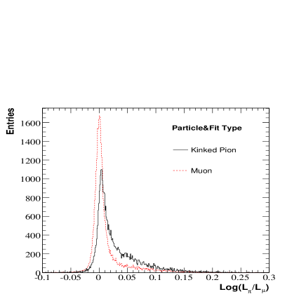
The $\mu/\pi$ separation provided by the kinked pion fitter is not as clean as the $\mu$/e separation. There is no single value of the likelihood ratio at which a cut could be placed that would reject a large population of muons while retaining a significant fraction of pions. The goal of this analysis, however, is to reconstruct events with both a muon and a pion present, and to determine the identity of each track. In that case, the separation power indicated by Fig. 1 is doubled due to the presence of the second track.

II.1.2 Kinematics Reconstruction Performance

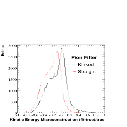
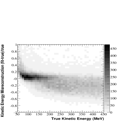
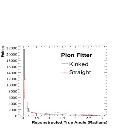
Although the main motivation for developing a kinked-track fitter was to provide a means for separating muons from charged pions, the improved modeling of pion trajectories results in superior event reconstruction as well. The fractional energy reconstruction bias (i.e. the ratio of the fit/true difference to the true value) from both the straight and kinked pion fitters is shown in Fig. 2. The straight pion fitter reconstructs pion energies 10% low, whereas the kinked fitter reconstruction bias peaks at zero. In addition, the “shoulder” just below the peak, where the reconstructed energy underestimates the true pion energy, is reduced by the kinked pion fitter. The two-dimensional plot of the fractional energy reconstruction bias versus the true energy in Fig. 3 shows that the shoulder comes from higher energy pions that can produce multi-kink events and cause larger pion energy losses at each kink. The pion direction reconstruction is also significantly improved with the kinked fitter, as shown in Fig. 4. The event population in the first few bins of the angle between the reconstructed and true directions are nearly doubled in the kinked fitter relative to the straight fitter.

Figure 2: The fractional pion kinetic energy reconstruction bias from the straight and kinked pion fits to Monte-Carlo-generated single pion events is shown. The low-energy shoulder is significantly reduced in the kinked fitter, and rather than being 10% low, as is the case with the straight fitter, the peak from the kinked fitter is centered at zero.

Figure 3: The fractional pion kinetic energy reconstruction bias is plotted versus the true energy for Monte-Carlo-generated single pion events. The low-fit-energy shoulder is caused by higher energy pions.

Figure 4: The angle between the reconstructed and true pion directions is shown for both straight and kinked pion fits to Monte-Carlo-generated single pion events. The population in the lowest few bins where the properly reconstructed events lie is nearly twice as large for the kinked fitter.

II.2 $\textrm{CC}\pi^{+}$ Fit

With the ability to reconstruct charged pions, a full $\textrm{CC}\pi^{+}$ fitter is formed by simultaneously fitting for a straight muon and a kinked pion track. A $\textrm{CC}\pi^{+}$ fit has 14 parameters: a common vertex (4 parameters), the initial energy and direction of both the muon and pion (6 parameters), and the additional kinked-track parameters for the pion (4 parameters). Just as in the kinked pion fitter, the predicted charges from all track segments (upstream pion, downstream pion, and muon) are summed to get the total predicted charge for each PMT.

II.2.1 $\textrm{CC}\pi^{+}$ Fit Seeding

Each $\textrm{CC}\pi^{+}$ event is assumed to have three Cherenkov rings from the three-track segments in the event: the upstream pion segment, the downstream pion segment, and the muon track. Each ring is found in succession using intermediate two- and three-track likelihood functions. The three tracks are then pieced together in several different pairings to create the kinked pion track and the straight muon track. The pairing that produces the best likelihood is used to seed the $\textrm{CC}\pi^{+}$ fitter.

The first of the three rings is found by performing a one-track fit. The results of the fit are frozen in place, and a scan for a second track is performed over 100 equally spaced directions. At each scan point, a two-track likelihood function is evaluated, and the configuration that gives the best likelihood value is used to seed a full two-track fit. This process is then repeated by freezing the result of the two-track fit and scanning for a third track using a three-track likelihood function. The result of the scan seeds a full three-track fit.

Once three tracks are found that characterize the Cherenkov rings in the event, they are combined to form a straight muon and a kinked pion. Only pairings where the downstream pion track has a lower energy than the upstream pion track are allowed. This reduces the number of possible groupings to three. Each of these three seeds is passed to the full $\textrm{CC}\pi^{+}$ fitter, and the fit that produces the best likelihood is chosen.

II.2.2 Fit Results

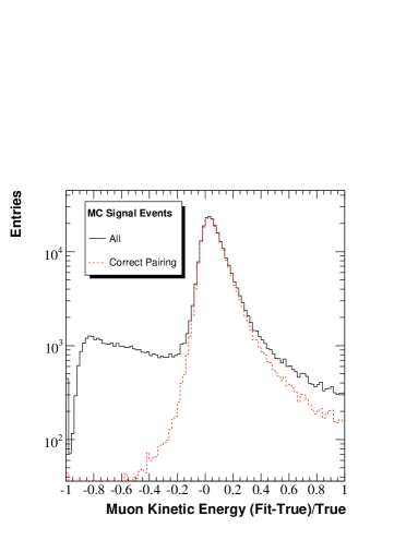
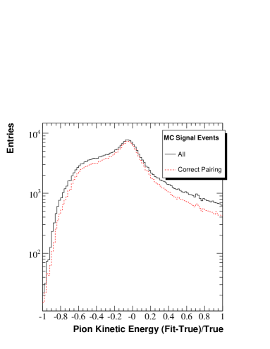
The fractional kinetic energy reconstruction bias distributions for the muon and pion tracks are given in Fig.s 5 and 6, respectively. The muon kinetic energy has a small tail at low reconstructed energy due to $\mu/\pi$ mispairing. The reconstructed pion kinetic energy has the same low-energy shoulder from high energy particles seen in the pion-only fit in Fig. 2. In addition, the fitter tends to place about 5% too much energy in the muon track at the expense of the pion track.

Figure 5: The fractional muon kinetic energy reconstruction bias is shown for all Monte Carlo signal events, and for correctly paired signal events after all cuts other than the $m_{\pi+N}$ cut. Most of the low-fit-energy tail is due to events where the pion was misidentified as the muon.

Figure 6: The fractional pion kinetic energy reconstruction bias is shown for all Monte Carlo signal events, and for correctly paired signal events after all cuts other than the $m_{\pi+N}$ cut. The low-reconstructed-energy shoulder from the pion-only fit in Fig. 2 is seen here as well.

While the pion energy fit is more accurate at low track energies, the opposite is true for the reconstructed pion direction. The track direction reconstruction relies on the existence of a well-defined Cherenkov ring from the upstream pion track segment. At MiniBooNE neutrino energies, 16% of the generated pion kinetic energy spectrum lies below 70 MeV. This corresponds to an above-Cherenkov propagation distance of less than 10 cm, which is often insufficient to determine the direction. For comparison, fewer than 1% of muons are generated below 70 MeV. In addition, the pion inelastic interaction length in mineral oil in the energy range of interest is approximately 1 m Ashery et al. (1981), which means 10% of all pions will have upstream segments shorter than 10 cm.

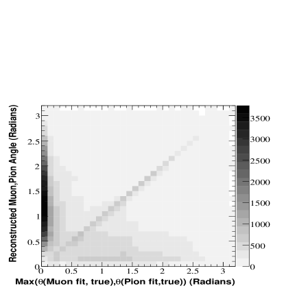
The ability of the fitter to correctly reconstruct both the muon and the pion directions is shown in Fig. 7. The reconstructed angle between the muon and pion is plotted against the larger of the two reconstructed/true angles. A perfect fitter would place all events in the lowest column where both reconstructed/true angles are zero. Fig. 7 shows that those bins contain the largest event population. The other significant event population is along the diagonal of the plot. These are events where the fitter has misidentified the muon as a pion and vice versa. In such cases, the angle between the true and reconstructed directions of both the muon and pion will be near the reconstructed $\mu/\pi$ angle. This is the first time charged pions have been tracked and their kinematics measured in a Cherenkov detector.

Figure 7: The reconstructed angle between the muon and pion directions for Monte Carlo $\textrm{CC}\pi^{+}$ events is shown versus the larger (i.e. worse reconstructed) of the two reconstructed/true angles: $\theta(\mu_{rec},\mu_{true})$ and $\theta(\pi_{rec},\pi_{true})$. The bins in the left-most columns represent events where both tracks have been properly reconstructed. Events in which the tracks have been misidentified appear along the diagonal.

II.2.3 Neutrino Energy

With reconstructed energies and directions for both the muon and pion, the energy of the incident neutrino can be determined. Assuming the target nucleon is at rest and the remaining, unmeasured final-state particle is a nucleon, the neutrino energy is specified by 4-momentum conservation,

$$E_{\nu}=\frac{m_{\mu}^{2}+m_{\pi}^{2}-2m_{N}(E_{\mu}+E_{\pi})+2p_{\mu}\cdot p_{\pi}}{2\left(E_{\mu}+E_{\pi}-\left|{\bf p}_{\mu}\right|\cos\theta_{\nu,\mu}-\left|{\bf p}_{\pi}\right|\cos\theta_{\nu,\pi}-m_{N}\right)},$$ (2)

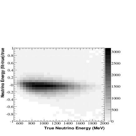
where $m_{x}$, $E_{x}$, $p_{x}$, and $\left|{\bf p}_{x}\right|$ are the mass, energy, 4-momentum, and 3-momentum magnitude of particle $x$ in the detector frame, and $\theta_{\nu,\mu}$($\theta_{\nu,\pi}$) is the angle between the directions of the muon(pion) and the neutrino. The neutrino direction is determined by the event vertex location and the mean neutrino emission point from the beam Monte Carlo prediction, although the large distance between the beam and the detector means this angle is never larger than one degree. The comparison between reconstructed and true neutrino energy is given in Fig. 8. The resolution is 13.5% over most of the sensitive range, with a slight increase at the highest energies.

Figure 8: The neutrino energy reconstruction bias is plotted against the true neutrino energy for Monte Carlo generated $\textrm{CC}\pi^{+}$ events. The reconstructed and true values are well correlated over the entire energy spectrum.

The decreased pion angular resolution at lower pion energies has little impact on the neutrino energy reconstruction since the neutrino energy calculation becomes less sensitive to the reconstructed pion direction as the pion energy is reduced. In addition, events with misidentified tracks that are otherwise well-reconstructed will produce nearly the same neutrino energy, since muons and pions have similar masses.

II.2.4 Invariant mass of the hadronic system

By making the aforementioned assumptions required to calculate the neutrino energy, the kinematics of the interaction are fully specified. Previous attempts to measure $\textrm{CC}\pi^{+}$ interactions by reconstructing only the muon required the additional assumption that the recoiling particle was an on-shell $\Delta$ baryon Wascko (2006). Since the width of the $\Delta$ resonance is about 10% of its mass, this assumption results in an irreducible contribution to the neutrino energy resolution. By measuring the pion kinematics, the $\Delta$ mass constraint can be removed.

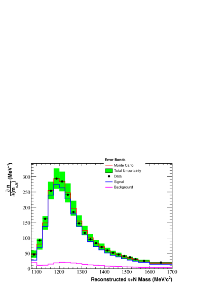
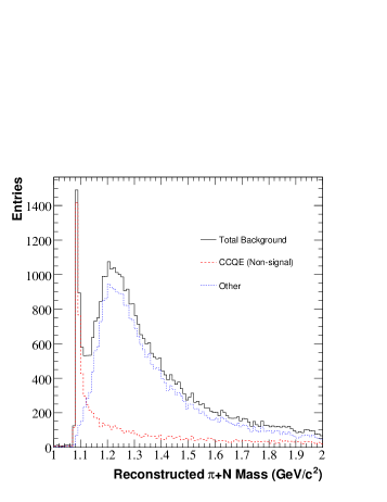
The absence of a $\Delta$ mass constraint also means that the $\pi^{+}+N$ invariant mass, which is dominated by the $\Delta$ resonance, can be measured. Fig. 9 shows the reconstructed $\pi^{+}+N$ mass, and a breakdown of the background composition is given in Fig. 10. The CCQE background features a sharp peak near threshold. CCQE interactions typically do not produce a pion, and the fitter correctly assigns very little kinetic energy to the hadronic system in these events.

Figure 9: The reconstructed $\pi+N$ mass distribution is shown for both the data and the Monte Carlo simulation with full systematic uncertainties. The MC distribution has been normalized to the data. The signal and background components of the Monte Carlo distribution are also shown. At MiniBooNE energies, the majority of $\textrm{CC}\pi^{+}$ events come from decays of the $\Delta(1232)$ resonance.

Figure 10: The reconstructed Monte Carlo $\pi^{+}$ +$N$ background distribution is divided into CCQE background events, and all other backgrounds. Since the CCQE events do not contain a pion, they are peaked near threshold ($m_{\pi}+m_{N}$).

II.2.5 Momentum Transfer

The final variable measured in this analysis is the 4-momentum transfer, $q$, from the leptonic current to the hadronic portion of the decay, which is characterized by its relativistic invariant,

$$Q^{2}\equiv-(p_{\mu}-p_{\nu})^{2}.$$ (3)

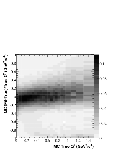
Since $Q^{2}$ is a property of the exchanged $W$ boson, it is completely specified by the change in the leptonic current. However, this also means that, unlike the neutrino energy calculation, the reconstructed $Q^{2}$ distribution is quite sensitive to $\mu/\pi$ misidentification. Fig. 11 shows the fractional error in the reconstructed $Q^{2}$ distribution, normalized in columns of true $Q^{2}$. Most of the columns peak near zero, but at high $Q^{2}$, a second population of events appears in which the fit underestimates the true $Q^{2}$. These events are dominated by a high energy muon that has been misidentified as a pion, giving the impression that most of the neutrino momentum was transferred to the hadronic system. After all analysis cuts, the $Q^{2}$ resolution is 18% below 0.3 GeV${}^{2}/c^{4}$ and 20% below 1 GeV ${}^{2}/c^{4}$.

Figure 11: The $Q^{2}$ (fit-true)/true distribution for Monte Carlo events is plotted versus the true $Q^{2}$. Each column of true $Q^{2}$ has been normalized to unity. The reconstruction is able to determine the true $Q^{2}$ over the full range of the measurement.

III Event Selection

MiniBooNE events are recorded in a 19.2 $\mu s$ time window beginning 4.6 $\mu s$ prior to the arrival of the 1.6 $\mu s$ beam pulse. The event time window is further subdivided into groups of PMT hits called subevents. The hit times in each subevent must have no more than two gaps longer than 10 ns and no gaps longer than 20 ns.

The first subevent in each event consists of the final-state particles produced in the neutrino interaction. Muons and pions can stop in the detector and decay to produce Michel electrons. These Michel electrons result in additional subevents that provide a simple and powerful tool for separating neutrino event types. CCQE events, which contain a muon in the final state, most often produce two subevents. Since $\textrm{CC}\pi^{+}$ events are more likely to produce two Michel electrons from the decays of the final-state muon and pion, events are required to have three subevents.

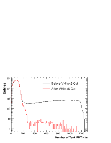
To remove backgrounds from cosmic rays, fewer than six hits are allowed in the veto region in all three subevents. The effect of this cut on the second subevent is shown in Fig. 12. If a cosmic muon enters the tank before the beginning of the event time window, it can stop and decay within the event time window to simulate a neutrino interaction. These events are removed by requiring a minimum number of PMT hits in the main tank in the first subevent. If this cut is placed at 200 hits, more than 99.9% of beam unrelated backgrounds are removed Aguilar-Arevalo et al. (2009c). For the present analysis, the tank hits requirement has been relaxed to 175 hits since it is unusual for a Michel electron event to produce three subevents. The second and third subevents are required to have between 20 and 200 hits in the main tank to accept subevents from Michel electrons.

Figure 12: The tank hits distribution in data is shown for the second subevent before and after requiring fewer than 6 hits in the veto. The Michel electron peak is mostly unaffected, while the large tail from entering comic rays is mostly removed.

To remove events that occur close to the edge of the detector, the muon and pion tracks are required to travel at least 150 cm before reaching the wall. Particle trajectories that begin near the edge of the tank and are directed toward the tank wall are poorly reconstructed since they are detected by a small number of PMTs. Conversely, events that occur just inside the tank wall but consist of tracks that all point toward the interior of the tank are well reconstructed. An illustration of this cut is given in Fig.s 13 and 14.

Figure 13: The distance between the tank wall and event vertex along the muon trajectory is shown for both data and Monte Carlo events. All other cuts have been applied and the error bars include only data statistics. The cut on this distribution removes all events below 150 cm.

Figure 14: The distance between the tank wall and event vertex along the pion trajectory is shown for both data and Monte Carlo events. All other cuts have been applied and the error bars include only data statistics. The cut on this distribution removes all events below 150 cm.

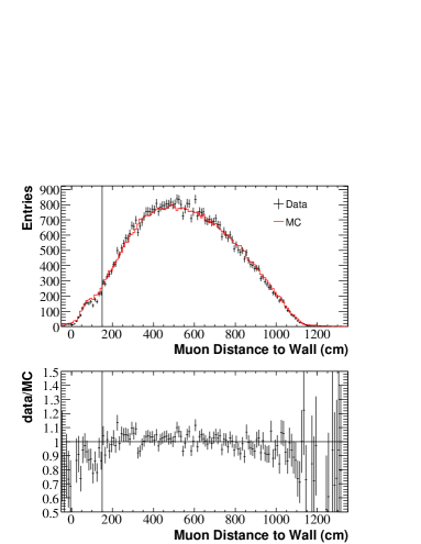
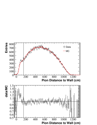
A final cut on the $\pi+N$ mass ($m_{\pi+N}$) is used to eliminated events where the final-state particles are misidentified. The fitter misreconstructs the muon as a pion, and vice versa, 21.4% of the time. In cases where a high energy muon is misreconstructed as a pion, the reconstructed kinematics give a spuriously high $m_{\pi+N}$. The relationship between the generated and reconstructed $m_{\pi+N}$ is shown in Fig. 15. Beyond reconstructed masses of 1350 MeV/c², the population of misreconstructed events begins to dominate, so a cut is implemented to remove these events. Fig. 16 shows the improvement in the reconstructed muon kinetic energy resulting from the $m_{\pi+N}$ cut. The properly reconstructed events are mostly retained while the tail at low reconstructed energy is greatly reduced.

A well-matched event is defined in terms of the angles between true and reconstructed tracks. There are four such angles: $\theta$(true $\mu$, fit $\mu$), $\theta$(true $\pi$, fit $\pi$), $\theta$(true $\mu$, fit $\pi$), $\theta$(true $\pi$, fit $\mu$). If the minimum of these four angles is between a true track and its corresponding reconstructed track, the event is said to be well-matched. This means that an event containing two properly reconstructed tracks is well-matched if the fitter correctly identifies the muon and pion tracks. Events where the direction of one of the tracks is misreconstructed (e.g. one track is below Cherenkov threshold) are still considered to be well-matched if the angle between the measured track and its corresponding true track is small. The fraction of well-matched events increases from 78.6% to 88.0% with the introduction of the $m_{\pi+N}<1350~{}\textrm{MeV}/\textrm{c}^{2}$ cut.

Figure 15: The Monte Carlo $m_{pi+N}$ distribution shows a correlation between the reconstructed and true distributions at low mass. At high reconstructed mass, the distribution is dominated by events with a high energy muon misidentified as a pion. A cut is placed at 1350 MeV/c² to remove these events.

Figure 16: The fractional muon kinetic energy reconstruction bias is shown for Monte Carlo $\textrm{CC}\pi^{+}$ events before and after the $m_{\pi+N}$ cut with all other cuts applied. The lower plot shows the fraction of events that pass the cut in each bin. The tail at low-fit-energy is significantly reduced.

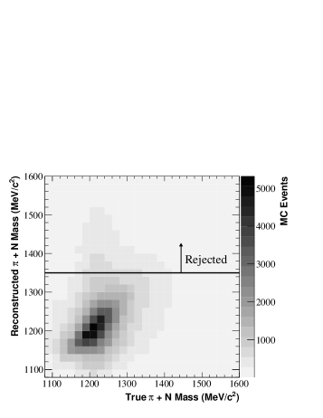
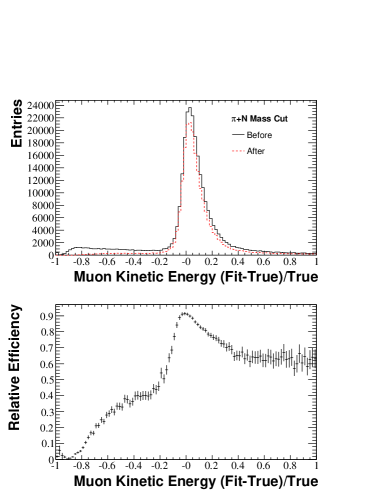
After all cuts, 48,322 events are seen in the data with an overall signal efficiency of 12.7%, and a purity of 90.0%. The background contributions are labeled according to the particles produced in the initial neutrino interaction (i.e. prior to any final-state effects), rather than the final state emerging from the nucleus. The largest backgrounds (listed by percentage of the total sample) are from CC multi-$\pi$ events (3.1%), CCQE events (2.7%), and $\textrm{CC}\pi^{+}$ events (1.3%) in which the pion content of the final state is altered via nuclear effects and are therefore not considered signal events. The complete lists of both signal and background compositions are given in Tables 1 and 2, respectively.

Table 1: The signal efficiency and purity are shown after each successive analysis cut. The efficiency is given relative to all interactions that occur within the detector, including the outer veto region; if restricted to events produced within 100 cm of the tank center, the effiency rises to 27%. A full list of efficiency and purity by NUANCE event type is given in Ref. Wilking (2009).

Cut #	Description	Effic.(%)	Purity (%)
1	no cuts	100	18.7
2	1st subevent, tank hits $>175$ and veto hits $<6$	47.5	23.6
3	number of subevents = 3	23.2	60.5
4	2nd and 3rd subevents: tank hits $<200$ and veto hits $<6$	19.6	86.3
5	muon and pion distance to wall $>150$ cm	16.9	87.2
6	$\pi+N$ mass $<1350~{}\textrm{MeV}/\textrm{c}^{2}$	12.7	90.0

Table 2: The composition of the background after all analysis cuts is given in terms of the NUANCE interaction mode (i.e. before final-state interactions). The total background is 10% of the final event sample. The background acceptance and contamination after each cut is given in Ref. Wilking (2009).

NUANCE Interaction	Initial State Description	Background Fraction (%)
CC multi-$\pi$	1 muon, $>$1 pion, and 1 nucleon	31.4
CCQE	1 muon and 1 proton	26.8
$\textrm{CC}\pi^{+}$	1 muon, 1 $\pi^{+}$, and $\leq$1 nucleon	13.4
$\textrm{CC}\textrm{meson}B$	1 muon, 1 non-$\pi$ meson, and 1 baryon	8.5
CCDIS	1 muon and multiple hadrons	6.6
$\textrm{CC}\pi^{0}$	1 muon, 1 $\pi^{0}$, and 1 proton	5.7
$\bar{\nu}$	all $\bar{\nu}$ interactions	1.1
other		6.5

IV Cross Section Measurements

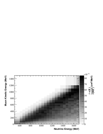
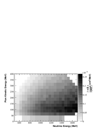
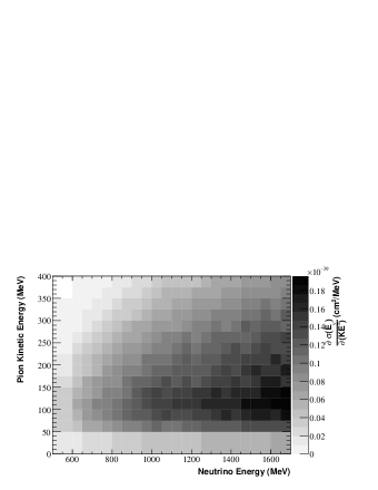
The observable $\textrm{CC}\pi^{+}$ analysis includes measurements of the cross section in terms of several kinematic variables. The integrated cross section has been measured as a function of neutrino energy. The other one-dimensional measurements are differential cross sections as a function of the muon and pion energies and $Q^{2}$. Since these one-dimensional measurements are necessarily averaged over the full neutrino energy spectrum, a corresponding two-dimensional measurement of each variable is made in bins of neutrino energy. In addition, the energy and direction are measured together for both the muon and pion in two double-differential cross section measurements.

IV.1 Data Unfolding

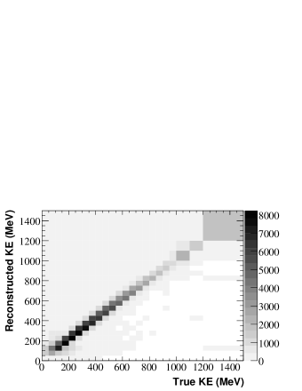
Because of biases and imperfect resolution in the event reconstruction, the event distributions measured in the data do not perfectly reflect the underlying true distributions. For example, as shown in Fig. 3, the pion energy reconstructed by the $\textrm{CC}\pi^{+}$ fitter is systematically high at low true energy, and falls below the true energy as the energy increases. Since such biases are modeled in the Monte Carlo simulation, it is possible to “unfold” these bin-migration effects.

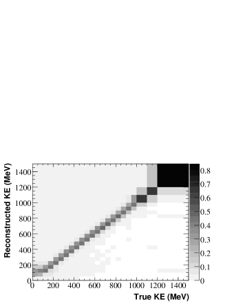
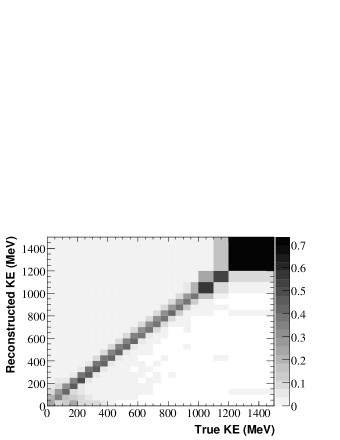
The Monte Carlo bin-migration matrix for a given variable, $v$, is constructed by forming a two-dimensional histogram of the reconstructed value of $v$ versus the true value, and normalizing each true column to unity as illustrated in Fig. 17. Each element, $F_{ji}$, in the bin-migration matrix represents the probability that an event generated with a value of $v$ in bin $i$ will be reconstructed in bin $j$. By definition,

$$N^{int}_{j}=\sum_{i}F_{ji}T_{i},$$ (4)

where $N^{int}_{j}$ is the reconstructed distribution and $T_{i}$ is the true distribution.

To produce an unfolding matrix, the reconstructed-versus-true histogram is, instead, normalized in reconstructed rows. This produces a matrix, $M_{ij}$, that performs the inverse operation of Eq. 4. This method, proposed by D’Agostini, avoids the problem of incorporating large statistical variance in the unfolding matrix, which is often an issue with inverting the bin-migration matrix D’Agostini (1995). The unfolding matrix can be extended to two-dimensional distributions in a straight forward way by arbitrarily ordering each of the two-dimensional bins and repeating the same process used in the one-dimensional case.

With the introduction of the unfolding matrix, $M_{ij}$, the full expression for the differential cross section can be written as

$$\frac{\partial\sigma}{\partial v}(v_{i})=\frac{\sum_{j}M_{ij}(D_{j}-B_{j})}{\epsilon_{i}\Delta v_{i}N_{targ}\Phi}.$$ (5)

where $v_{i}$ is the variable to be measured in true bin $i$, $D_{j}$ is the measured data distribution in reconstructed bin $j$, $B_{j}$ is the predicted background distribution, $\epsilon_{i}$ is the efficiency, $\Delta v_{i}$ is the width of bin $i$, $N_{targ}$ is the number of target molecules in the fiducial volume, and $\Phi$ is the integrated flux in units of neutrinos per unit area, as described in Sec. IV.4.

Figure 17: The reconstructed-versus-true (top), bin-migration (middle), and unfolding (bottom) matrices are shown for muon kinetic energy. The bin-migration matrix is formed by normalizing the true columns of the Monte Carlo reconstructed-versus-true matrix to unity, while the unfolding matrix is formed by normalizing the reconstructed rows.

IV.2 Unfolding Bias

Although the use of $M_{ij}$ rather than $F_{ij}^{-1}$ avoids the statistical variance issues involved with matrix inversion, it does introduce some bias. In general, unfolding procedures often require the introduction of some amount of bias in order to reduce the statistical variances associated with matrix inversion such that the overall uncertainty is reduced D’Agostini (1995). Since the bin-migration matrix, $F_{ij}$, is normalized in columns of the true distribution, $F_{ij}$ and $F_{ij}^{-1}$ are fully independent of the true Monte Carlo distribution, and are therefore unbiased transformations. The $M_{ij}$ matrix is normalized in reconstructed rows, which means any change to the shape of the true distribution slice within a reconstructed bin (i.e. changes to the Bayesian prior probabilities as described in Ref. D’Agostini (1995)) will result in the reconstructed events in that bin being assigned to the true bins in different proportions.

To quantify the size of the unfolding bias, an iterative technique is used. The background-subtracted, unfolded data provide an inferred true distribution as described in Section IV.1. Each Monte Carlo event is then assigned a weight given by the binned ratio of inferred true data to the true Monte Carlo simulation. Using these weights, a new reconstructed-versus-true histogram is created from which a new $M_{ij}$ unfolding matrix is formed. The data distribution is unfolded again using the new unfolding matrix and the processes is repeated.

Successive iterations of the inferred data distribution have two distinct features in both the one- and two-dimensional cases. The first is that the largest excursion relative to the uniterated inferred distribution is in the first iteration. The other is that each successive iteration oscillates about an intermediate preferred value, which is a convolution of the true underlying distribution and any systematic biases in the unfolding matrix. The amplitude of these oscillations decreases as the number of iterations increases. The size of the largest systematic variation, the first iteration, is taken as the systematic uncertainty.

IV.3 Efficiency Correction

After the data are unfolded, the inferred true data distribution is corrected for events lost due to data selection cuts and detector inefficiency. The numerator of the efficiency correction is the true distribution of all Monte Carlo events that pass the cuts. The denominator is the generated Monte Carlo distribution, formed before any cuts are imposed. The ratio of these two distributions gives the fraction of events in a particular bin that survive the analysis cuts,

$$\epsilon_{i}=\frac{N_{i}^{true~{}after~{}cuts}}{N_{i}^{generated}}.$$ (6)

The efficiency is insensitive to changes in the underlying physical parameters used to produce the generated distribution. If any portion of the generated distribution is incorrectly enhanced, a proportional effect should be seen in the true distribution and thus cancel in the efficiency.

Monte Carlo events are generated out to a radius of 610.6 cm to include all neutrino interactions in the main tank, the veto region, and the tank wall. Since the measurement being performed is a neutrino cross section in mineral oil, all other materials must be excluded in forming the generated Monte Carlo distribution. To avoid the PMTs and, in particular, the material voids inside the PMTs, the efficiency denominator is formed from a subset of these events generated within a radius of 550 cm.

Nearly all of the events generated outside of 575 cm are removed by the veto hits cut; however, there will be a population of events generated between 550 cm and 575 cm that pass all cuts, particularly in the upstream portion of the tank. The extra contribution from events in the 550-575 cm shell are in good agreement in the reconstructed data and Monte Carlo vertex distributions.

The number of interaction targets in the cross section formula, $N_{targ}$, corresponds to the definition of the generated volume used in the efficiency calculation. To extract the number of targets from the volume, the only experiment-dependent quantity needed is the oil density, which has been measured to be $0.845\pm 0.001~{}\textrm{g}/\textrm{cm}^{3}$ Aguilar-Arevalo et al. (2009c). Since the cross section only depends on the relative amount of each atomic species, the interaction target is chosen to be an average single unit on the hydrocarbon chain, CH_2.08.

IV.4 Flux Factor

The flux factor, $\Phi$, in Eq. 5 takes the form of either a distribution in neutrino energy or a single value, depending on the type of cross section measurement being performed. For measurements binned in $E_{\nu}$, the flux factor is the number of incident neutrinos per unit area in each measured bin. These measurements are flux-averaged over the width of each bin. In the differential and double-differential cross section measurements, the flux factor is the fully integrated neutrino flux, and the cross section is flux-averaged over the entire neutrino energy spectrum. The total integrated $\nu_{\mu}$ flux factor for the MiniBooNE experiment, normalized to protons on target (POT), is $5.19\times 10^{-19}$ ($\nu_{\mu}$/cm²/POT).

Flux-averaged differential cross section measurements implicitly contain the shape of the neutrino energy spectrum, which must also be reported to fully specify the results. To mitigate the dependence on the experiment-dependent shape of the energy spectrum, each of the differential cross section measurements has also been performed in bins of neutrino energy.

IV.5 Systematic Uncertainties

The systematic uncertainties are grouped by error sources. Each source is a set of correlated uncertainties from a particular stage of the simulation. The parameters of each error source are related by an error matrix from which a set of correlated parameter variations, called a “multisim,” can be drawn. Each new set of parameters produces a systematically varied version of any reconstructed distribution. The spread in the reconstructed multisim distributions is used to calculate the total systematic uncertainty.

There are two distinct types of systematic variations. Some systematics, such as the flux and cross section uncertainties, only affect the probability with which an event will occur. For this type of uncertainty, a systematically varied distribution can be produced by reweighting the central value Monte Carlo distribution. Each event is multiplied by the ratio of the event probability calculated with the systematically varied set of parameters to the central value event probability.

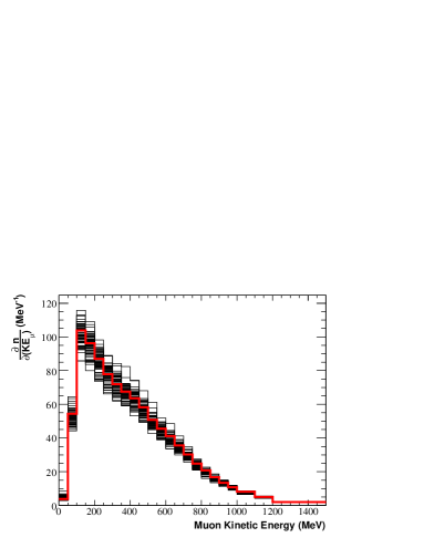
The other type of systematic variation affects the measured properties of the event after it is produced, such as the amount of light generated as a function of wavelength and the propagation of the light through the oil. In general, these variations cannot be accomplished via reweighting. Instead, these errors are determined using 67 data-sized Monte Carlo simulations that are generated using parameter draws from the optical model error matrix. A plot of these optical model multisims in muon kinetic energy is shown in Fig. 18.

Figure 18: The reconstructed muon kinetic energy is plotted in each of the 67 optical model multisims. The central value Monte Carlo distribution (red) is overlayed for comparison.

.

IV.5.1 Error Matrices

The uncertainties in the measured cross sections are described by an error matrix that characterizes the correlated uncertainties in the measured values in each bin. For each error source, an error matrix, $E_{ij}^{source}$, is calculated from the bin population differences in the multisims compared to the central value,

$$E_{ij}^{source}=\frac{1}{N}\sum_{m=1}^{N}\left(n_{m,i}-n_{CV,i}\right)\left(n_{m,j}-n_{CV,j}\right),$$ (7)

where $N$ is the number of multisims, $n_{m,i}$ is the number of events in bin $i$ of multisim $m$, and $n_{CV,i}$ is the number of events in bin $i$ in the central value Monte Carlo simulation. Once an error matrix has been calculated for each source, the total error matrix is given by summing each component matrix.

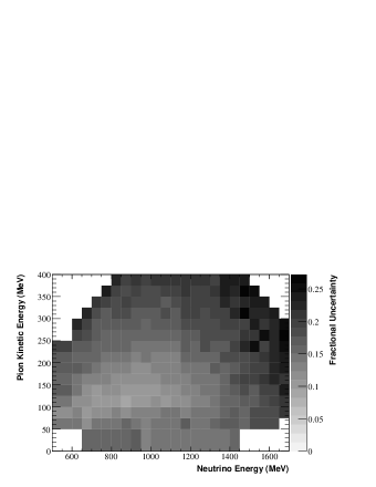
Since the statistical fluctuations in a particular bin are unrelated to the fluctuations in any other bin, statistical error matrices are always diagonal. By design, these uncertainties are built into the optical model error matrix since each optical model multisim was constructed to have the same number of events as the data. Unfortunately, this also has the effect of adding statistical fluctuations to the off-diagonal terms. As more optical model multisims are incorporated into the calculation of the error matrix, the size of these spurious fluctuations is decreased. The fluctuations are also smaller for bins with significant event populations. For this reason, cross section results will only be reported for bins with at least 25 unfolded data events. In the one-dimensional cross section measurements, the event populations are large enough that this effect is negligible. The reweighting multisims do not suffer from this effect.

To evaluate the systematic uncertainties in the cross section, the full cross section calculation procedure outlined in Eq. 5 is performed in each multisim. The multisim distributions replace the corresponding central value distributions in the calculation. The reconstructed data distribution remains the same, but multisim distributions are used for the unfolding matrix, the background prediction, and the signal efficiency. The formula for the differential cross section with multisim dependent quantities explicitly identified is

$$\frac{\partial\sigma^{m}}{\partial v}(v_{i})=\frac{\sum_{j}M^{m}_{ij}(D_{j}-B^{m}_{j})}{\epsilon^{m}_{i}\Delta v_{i}N_{targ}\Phi^{m}},$$ (8)

where $m$ is the multisim index.

The results presented in the remainder of this report will list only the diagonal errors on each bin. The full error matrices for each distribution are quite large, and in the case of the two-dimensional measurements, they can contain over one million elements.

IV.5.2 Flux Uncertainties

The predicted neutrino spectrum is modified to correspond to the systematically varied flux parameters in each multisim. The diagonal uncertainties of the flux variations are shown in Fig. 19.

Figure 19: The $\nu_{\mu}$ energy spectrum is shown (top) along with the fractional flux errors (bottom). The fractional errors are cumulative such that each successive error band includes a quadrature sum of the previous errors such that the outer band gives the total error. A numerical description of the energy spectrum is given in Table 19

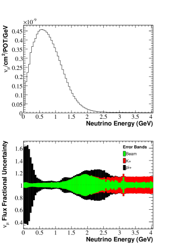
The largest of the flux errors is the uncertainty in the beam $\pi^{+}$ production in proton-beryllium interactions. The differential cross section for these interactions is parametrized using an empirical model from Sanford and Wang Sanford and Wang (1967). The parameters are determined in a simultaneous fit to data from the HARP and E910 experiments Catanesi et al. (2007); Chemakin et al. (2008). The flux prediction is not tuned in any way to data from MiniBooNE. As described in Ref. Aguilar-Arevalo et al. (2009b), the shape of the Sanford-Wang parametrization is not fully compatible with the data, but it is still used in the Monte Carlo simulation to provide physical constraints such as driving the cross section to zero at vanishing pion momentum. To determine the uncertainties in the pion production, the HARP data are fit with a spline function, and the resulting fit parameters are systematically varied according to the error matrix returned by the fit. The covariance of these spline function variations with respect to the Sanford-Wang central value are used to form the beam $\pi^{+}$ production error matrix as described in Ref. Aguilar-Arevalo et al. (2010a). This produces an uncertainty given by the HARP data errors in regions where the Sanford-Wang parametrization agrees with the spline function, and increases the errors in regions where they differ.

The portion of the flux relevant to observable $\textrm{CC}\pi^{+}$ interactions occurs at neutrino energies larger than about 400 MeV. For the peak neutrino energies (0.5-1 GeV), the beam $\pi^{+}$ flux uncertainties are around 8%. At higher neutrino energies, the beam $\pi^{+}$ uncertainty grows to as large as 25%. The beam $\pi^{+}$  fluctuations also exhibit very distinct features in shape. The residual effect of the wiggling behavior of the spline fit to the HARP data is apparent. In particular, the low-energy flux exhibits very large systematic excursions since there are no HARP data to constrain the fits in that region.

The other two flux related error sources have a smaller effect on the total uncertainty. The “Beam” uncertainties, which contain all systematic effects involving the proton beam and horn, are generally around the 5% level below 1 GeV and then expand at higher neutrino energies. The main contributor at high energies is the horn current skin depth uncertainty, which causes a $\sim$15% effect between 1.5 and 2.5 GeV. The $K^{+}$ production uncertainties are mostly irrelevant for this analysis. $K^{+}$ mesons become the dominant source of $\nu_{\mu}$ production at 2.3 GeV, and the uncertainties become dominant at neutrino energies greater than 2.5 GeV, where the flux is very small.

For the measurements not involving neutrino energy, the cross section calculation is only affected by the uncertainty in the integrated flux. The size of these variations for each of the flux error sources is given in Table 3.

Table 3: The uncertainties in the integrated flux are given for each of the flux error sources.

Error Source	Integrated Flux Uncertainty
$\pi^{+}$	10.4%
Beam	4.1%
$K^{+}$	0.4%

IV.6 Results

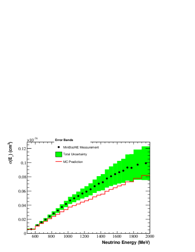
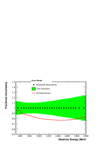
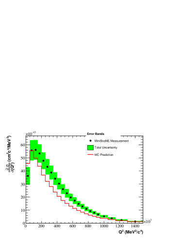
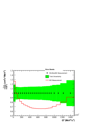
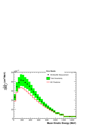
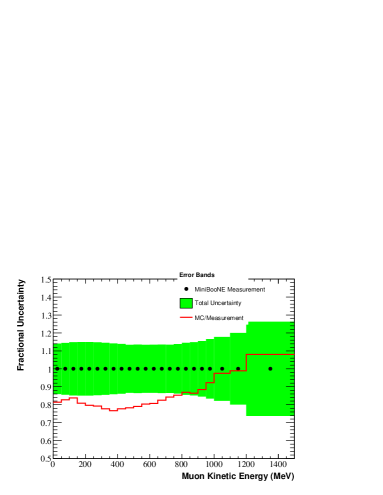
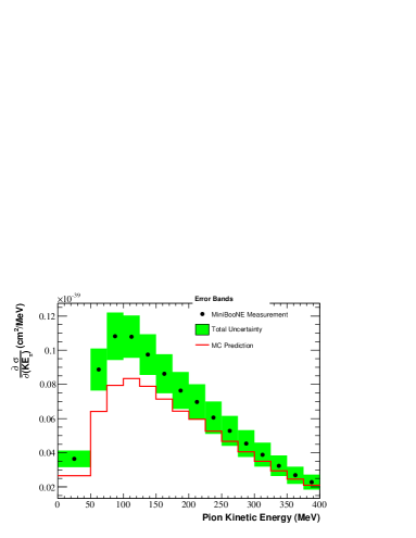
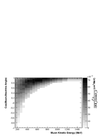
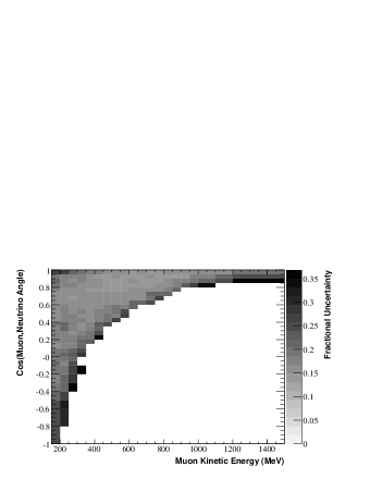
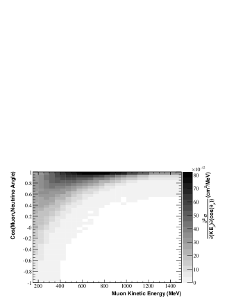
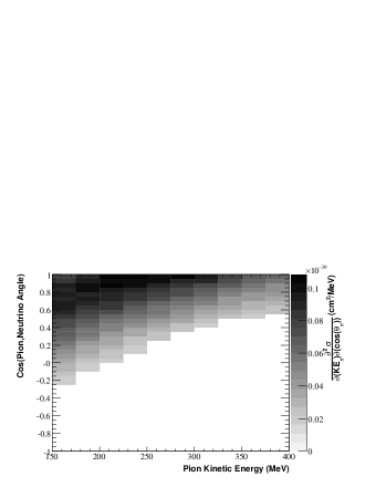
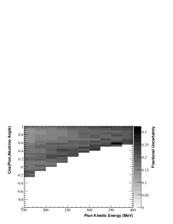
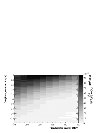
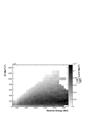
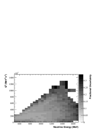
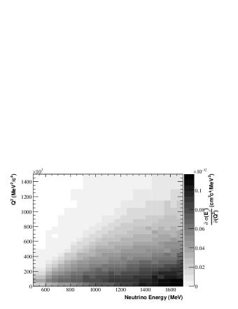
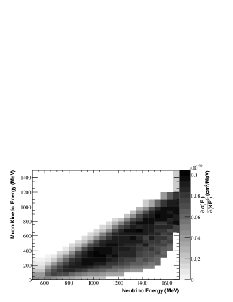
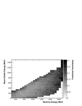
The observable $\nu_{\mu}\textrm{CC}\pi^{+}$ cross section on a CH_2.08 target has been measured in a variety of forms: a total cross section as a function of neutrino energy (Fig. 20), a differential cross section in $Q^{2}$ (Fig. 21), differential cross sections in the kinetic energy of the muon (Fig. 22) and the pion (Fig. 23), double-differential cross sections in the muon kinetic energy and angle (Fig. 24) and the pion kinetic energy and angle (Fig. 25), and two-dimensional measurements of each of the differential cross sections in bins of neutrino energy to provide results independent of the MiniBooNE energy spectrum (Fig.s 26, 27, and 28). This is the first time model-independent differential cross sections have been provided for the muon and pion kinematics in these interactions.

The binning for each of the one-dimensional distributions has been chosen such that the true Monte Carlo prediction in each bin exceeds 250 events after all cuts. The one-dimensional bin sizes are used for the two-dimensional measurements as well to retain sufficient precision in the most interesting regions of phase space. This results in several bins with very small numbers of predicted events. The data-sized optical model multisims produce unreliable uncertainties in bins with small event populations, and therefore results will only be reported for bins that contain at least 25 inferred true data events.

Table 4: The uncertainties in the total, flux-averaged cross section are given for the dominant error sources.

Error Source	Cross Section Uncertainty
Beam $\pi^{+}$ Production	9.2%
$\nu$ Cross Sections	8.2%
Proton Beam and Horn	4.3%
Optical Model	1.5%
Other	$<$3%

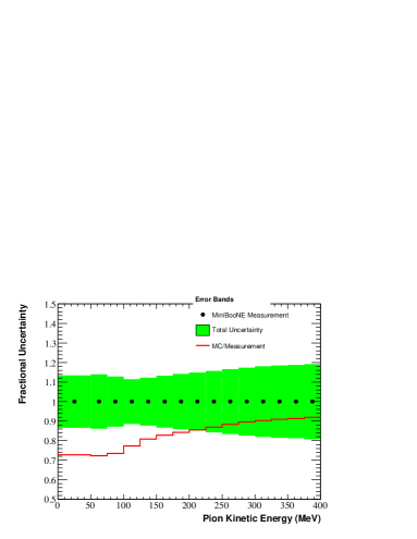
The uncertainties from the most significant error sources in the total cross section, averaged over the neutrino energy spectrum, are shown in Table 4. In each of the one-dimensional differential cross section measurements, the two largest sources of uncertainty are the beam $\pi^{+}$ production and the neutrino interaction cross sections. The $\pi^{+}$ production uncertainties in the flux-averaged results are dominated by the large uncertainties at low neutrino energy. Since the low-energy region has relatively little impact on the measurements binned in neutrino energy, the beam $\pi^{+}$  production uncertainties are is significantly lower and generally remain below 10% except at the highest neutrino energies.

The largest effects in the cross section uncertainties are pion absorption and charge-exchange interactions that take place after the pion has left the target nucleus. If the pion is absorbed, it will not produce a Michel electron and the event will fail the three-subevent requirement; therefore, pion absorption and charge-exchange interactions will directly affect the cut efficiencies. A 50% uncertainty is assigned to the pion charge-exchange cross section and a 35% uncertainty is assigned to pion absorption based on the agreement between the GCALOR Monte Carlo simulation Zeitnitz and Gabriel (1994) and external data Ashery et al. (1981); Jones et al. (1993); Ransome et al. (1992). The remainder of the cross section uncertainty is due to variations in the interaction cross sections of each background process.

Since the cross section measurements in Q² and neutrino energy include contributions from the incident neutrino, they must be unfolded back to the initial neutrino interaction, and are therefore dependent on the modeling of nuclear effects. In particular, additional uncertainties in the kinematics of the target nucleons are absorbed in these results. Conversely, the measurements in the muon and pion kinematic variables are properties of only the final, post-nuclear state, and are therefore largely insensitive to nuclear model uncertainties.

Finally, for most of the measured phase space, the uncertainty due to unfolding bias is negligible; however, it becomes significant at low $Q^{2}$ in both the one- and two-dimensional measurements. This particular region has two features that generally make unfolding difficult. The first is that the shape is rapidly changing, which strongly affects bin migration. Also, this is a region where the shapes in the data and Monte Carlo simulation significantly disagree, which increases the probability that the shape of the true $Q^{2}$ distributions within each reconstructed bin are incorrect. Despite these features, the unfolding uncertainty is still not the dominant systematic effect, and is of comparable size only in the few bins at low $Q^{2}$ which are susceptible to these effects.

Figure 20: The $\sigma(E_{\nu})$ measurement is shown with cumulative systematic errors. The absolutely normalized Monte Carlo prediction is shown for comparison. The bottom plot shows the fractional uncertainties and the ratio of the Monte Carlo prediction to the measurement.

Figure 21: The $\partial\sigma/\partial(Q^{2})$ measurement is shown with cumulative systematic errors. The absolutely normalized Monte Carlo prediction is shown for comparison. The bottom plot shows the fractional uncertainties and the ratio of the Monte Carlo prediction to the measurement.

Figure 22: The $\partial\sigma/\partial(KE_{\mu})$ measurement is shown with cumulative systematic errors. The absolutely normalized Monte Carlo prediction is shown for comparison. The bottom plot shows the fractional uncertainties and the ratio of the Monte Carlo prediction to the measurement.

Figure 23: The $\partial\sigma/\partial(KE_{\pi})$ measurement is shown with cumulative systematic errors. The absolutely normalized Monte Carlo prediction is shown for comparison. The bottom plot shows the fractional uncertainties and the ratio of the Monte Carlo prediction to the measurement.

Figure 24: The measured $\partial^{2}\sigma/\partial(cos(\theta_{\mu,\nu}))\partial(KE_{\mu})$ values are shown (top) along with the total fractional uncertainties (middle). Empty bins indicate regions where no measurement has been made. The Monte Carlo predicted cross section is shown for comparison (bottom).

Figure 25: The measured $\partial^{2}\sigma/\partial(cos(\theta_{\pi,\nu}))\partial(KE_{\pi})$ values are shown (top) along with the total fractional uncertainties (middle). Empty bins indicate regions where no measurement has been made. The Monte Carlo predicted cross section is shown for comparison (bottom).

Figure 26: The measured $\partial\sigma(E_{\nu})/\partial(Q^{2})$ values are shown (top) along with the total fractional uncertainties (middle). Empty bins indicate regions where no measurement has been made. The Monte Carlo predicted cross section is shown for comparison (bottom).

Figure 27: The measured $\partial\sigma(E_{\nu})/\partial(KE_{\mu})$ values are shown (top) along with the total fractional uncertainties (middle). Empty bins indicate regions where no measurement has been made. The Monte Carlo predicted cross section is shown for comparison (bottom).

Figure 28: The measured $\partial\sigma(E_{\nu})/\partial(KE_{\pi})$ values are shown (top) along with the total fractional uncertainties (middle). Empty bins indicate regions where no measurement has been made. The Monte Carlo predicted cross section is shown for comparison (bottom).

V Conclusion

Results have been presented for the observable $\textrm{CC}\pi^{+}$ cross section as a function of several fundamental kinematic variables. Of these results, the cross sections measured as a function of the neutrino energy are the least experiment dependent, since the predicted neutrino flux has been accounted for separately in each bin. Previous measurements of the neutrino energy cross section below 2 GeV have uncertainties larger than 20%, upon which the present results provide a significant improvement.

The present measurement is on average 23% higher than the NUANCE prediction for the observable cross section, which is compatible with some previous results, most notably Ref. Kitagaki et al. (1986). However, a direct comparison to past data is difficult since previous cross section measurements in this energy range were conducted on hydrogen or deuterium. Since MiniBooNE employs a nuclear target, it is unclear if the source of discrepancy seen in the current results lies in the single nucleon cross section, or whether it is due to nuclear effects.

The remaining kinematic $\textrm{CC}\pi^{+}$ cross sections have not been reported previously. Since the single- and double-differential cross section measurements are necessarily averaged over the shape of the neutrino flux prediction given in Fig. 19, each measurement of a final-state kinematic quantity has also been measured in bins of neutrino energy to remove the dependence on the MiniBooNE energy spectrum. The integrated one-dimensional measurements have also been included due to the familiarity of many in the community with flux-averaged results. This is the most complete set of information that has ever been available for $\textrm{CC}\pi^{+}$ on nuclear targets.

Appendix A Cross Section Tables

Tables 5-18 give the numerical values of each measured cross section and Table 19 gives the MiniBooNE $\nu_{\mu}$ flux prediction.

Table 5: The $\sigma(E_{\nu})$ results from Fig. 20 are given with the total uncertainty. Each row is a bin of neutrino energy (MeV) labeled according to its low edge.

Bin (MeV)	Result $(10^{-39}\textrm{cm}^{2})$
500	6.1 $\pm$ 0.8
600	11.5 $\pm$ 1.3
650	15.8 $\pm$ 1.7
700	19.6 $\pm$ 2.1
750	24.1 $\pm$ 2.5
800	28.3 $\pm$ 2.9
850	32.5 $\pm$ 3.3
900	37.3 $\pm$ 3.9
950	41.6 $\pm$ 4.4
1000	46.6 $\pm$ 5.0
1050	49.7 $\pm$ 5.6
1100	52.9 $\pm$ 6.1
1150	56.3 $\pm$ 7.0
1200	59.1 $\pm$ 7.6
1250	62.3 $\pm$ 8.4
1300	66.7 $\pm$ 9.4
1350	70.3 $\pm$ 10.5
1400	72.3 $\pm$ 11.4
1450	77.6 $\pm$ 12.8
1500	80.8 $\pm$ 13.9
1550	83.7 $\pm$ 14.9
1600	86.4 $\pm$ 15.9
1650	88.5 $\pm$ 16.9
1700	93.0 $\pm$ 18.5
1750	92.6 $\pm$ 19.3
1800	97.1 $\pm$ 21.4
1900	99.2 $\pm$ 23.7

Table 6: The $\partial\sigma/\partial(KE_{\pi})$ results from Fig. 23 are given with the total uncertainty. Each row is a bin of pion kinetic energy (MeV) labeled according to its low edge.

Bin (MeV)	Result $(10^{-41}\textrm{cm}^{2}/\textrm{MeV})$
0	3.6 $\pm$ 0.5
50	8.9 $\pm$ 1.2
75	10.8 $\pm$ 1.4
100	10.8 $\pm$ 1.2
125	9.7 $\pm$ 1.2
150	8.6 $\pm$ 1.1
175	7.6 $\pm$ 1.1
200	7.0 $\pm$ 1.0
225	6.1 $\pm$ 1.0
250	5.3 $\pm$ 0.9
275	4.5 $\pm$ 0.8
300	3.9 $\pm$ 0.7
325	3.2 $\pm$ 0.6
350	2.7 $\pm$ 0.5
375	2.3 $\pm$ 0.4

Table 7: The $\partial\sigma/\partial(Q^{2})$ results from Fig. 21 are given with the total uncertainty. Each row is a bin of $Q^{2}$ (GeV²/c⁴) labeled according to its low edge.

Bin (GeV2/c4)	Result $(10^{-45}\textrm{cm}^{2}c^{4}/\textrm{MeV}^{2})$
0.00	36.2 $\pm$ 6.7
0.05	55.8 $\pm$ 7.8
0.10	56.1 $\pm$ 7.5
0.15	53.4 $\pm$ 7.0
0.20	47.8 $\pm$ 6.4
0.25	43.2 $\pm$ 5.9
0.30	38.8 $\pm$ 5.3
0.35	34.1 $\pm$ 4.8
0.40	30.3 $\pm$ 4.3
0.45	26.1 $\pm$ 3.7
0.50	22.9 $\pm$ 3.3
0.55	19.8 $\pm$ 2.9
0.60	17.3 $\pm$ 2.5
0.65	14.8 $\pm$ 2.1
0.70	12.9 $\pm$ 1.9
0.75	11.0 $\pm$ 1.7
0.80	9.3 $\pm$ 1.4
0.85	8.0 $\pm$ 1.3
0.90	6.8 $\pm$ 1.1
0.95	5.3 $\pm$ 1.0
1.05	3.9 $\pm$ 0.7
1.15	2.5 $\pm$ 0.5
1.30	1.4 $\pm$ 0.4

Table 8: The $\partial\sigma/\partial(KE_{\mu})$ results from Fig. 22 are given with the total uncertainty. Each row is a bin of muon kinetic energy (MeV) labeled according to its low edge.

Bin (MeV)	Result $(10^{-42}\textrm{cm}^{2}/\textrm{MeV})$
0	23.1 $\pm$ 3.2
50	34.4 $\pm$ 5.0
100	39.0 $\pm$ 5.8
150	41.6 $\pm$ 6.2
200	41.2 $\pm$ 6.1
250	39.0 $\pm$ 5.7
300	37.3 $\pm$ 5.4
350	35.0 $\pm$ 4.9
400	32.0 $\pm$ 4.4
450	28.8 $\pm$ 3.8
500	26.1 $\pm$ 3.5
550	23.2 $\pm$ 3.1
600	20.8 $\pm$ 2.8
650	18.6 $\pm$ 2.5
700	15.9 $\pm$ 2.1
750	14.2 $\pm$ 2.0
800	12.3 $\pm$ 1.8
850	10.7 $\pm$ 1.6
900	9.3 $\pm$ 1.4
950	7.7 $\pm$ 1.3
1000	5.9 $\pm$ 1.0
1100	4.3 $\pm$ 0.8
1200	2.2 $\pm$ 0.6

Table 9: The $\partial\sigma(E_{\nu})/\partial(Q^{2})$ results from Fig. 26 are shown ($10^{-44}\textrm{cm}^{2}c^{4}/\textrm{MeV}^{2}$). Each bin is labeled according to its low edge. The columns are bins of neutrino energy (MeV) and the rows are bins of $Q^{2}$ (GeV²/c⁴). Empty bins indicate regions where no measurement has been made.

Bin	500	600	650	700	750	800	850	900	950	1000	1050	1100	1150	1200	1250	1300	1350	1400	1450	1500	1550	1600	1650
1.15																	1.1	1.0	1.2
1.05														0.9	1.1	1.2	1.5	1.8	1.8
0.95													1.1	1.4	1.7	2.0	2.2	2.3	2.3	2.6	3.1	3.1
0.90													1.6	2.0	2.0	2.3	2.4	2.8	3.4
0.85											1.2	1.5	1.8	2.2	2.6	2.8	2.8	3.1	3.5
0.80										1.1	1.6	2.0	2.6	2.7	2.9	3.4	3.4	3.4	3.8
0.75										1.8	2.2	2.5	2.7	3.2	3.4	3.5	3.8	4.6	4.3	4.8
0.70									1.6	2.2	2.6	2.9	3.2	3.4	3.8	4.0	4.3	4.5	5.5	5.0	5.1
0.65								1.7	2.2	2.7	2.9	3.1	4.0	3.6	4.1	4.7	4.8	5.2	5.2	5.6	5.3
0.60							1.4	2.4	2.4	3.3	3.7	4.1	4.2	4.5	5.2	5.4	5.2	5.0	5.9	6.0	5.6	6.3
0.55						1.3	1.9	2.4	3.0	3.8	4.1	4.6	4.7	5.2	5.1	5.7	5.6	6.1	5.8	7.0	7.4	7.6	7.4
0.50						1.8	2.4	3.2	3.6	4.4	4.8	5.4	5.6	5.8	5.8	6.7	6.6	6.6	7.0	6.2	7.5	7.3	7.1
0.45					1.5	2.3	3.1	4.0	4.7	5.2	5.7	5.5	6.1	6.5	6.4	6.6	6.9	7.7	7.1	7.4	6.6	7.9	8.1
0.40				1.3	2.5	3.2	4.2	4.8	5.1	6.1	6.5	6.7	6.7	7.1	7.1	7.3	7.5	7.1	8.1	7.9	8.6	8.4	9.3
0.35			1.1	2.0	3.1	4.0	4.8	5.7	6.4	6.8	6.8	7.0	7.4	7.8	7.6	8.2	8.1	8.1	8.7	9.1	8.7	8.9	8.8
0.30			1.9	3.1	4.1	5.1	6.0	6.1	7.4	7.4	7.4	8.0	8.0	8.1	8.6	9.1	9.2	9.0	8.7	8.7	8.9	8.7	9.8
0.25		1.8	3.0	4.1	5.3	5.9	6.7	6.8	7.5	7.7	8.2	8.2	8.1	8.5	9.0	9.0	9.8	9.4	9.4	8.8	9.5	9.7	10.1
0.20	1.0	2.9	4.2	5.2	6.0	6.7	6.9	7.6	8.0	8.8	8.5	8.8	8.7	9.3	9.2	9.5	9.6	9.5	9.9	10.3	10.2	11.5	11.2
0.15	1.9	4.1	5.4	6.3	7.1	7.4	7.5	8.3	8.7	9.1	9.0	9.3	9.2	9.6	9.4	9.6	9.6	9.9	10.6	11.6	10.8	11.2	10.3
0.10	3.1	5.2	6.6	7.0	7.4	7.6	7.9	8.7	8.2	9.2	9.3	9.4	9.5	9.1	9.0	9.5	9.2	9.5	10.4	9.4	10.5	10.2	9.8
0.05	4.3	6.0	6.5	7.0	7.3	7.4	7.6	8.0	7.9	8.0	8.0	8.3	8.6	8.2	8.6	8.2	8.4	7.8	8.6	9.3	9.3	9.6	10.0
0.00	1.9	2.7	3.3	3.6	3.9	4.3	4.6	4.8	5.2	5.4	5.4	5.2	5.8	5.9	6.0	6.4	6.6	6.1	6.3	6.7	7.2

Table 10: The percent uncertainty of the $\partial\sigma(E_{\nu})/\partial(Q^{2})$ results from Fig. 26 is shown. Each bin is labeled according to its low edge. The columns are bins of neutrino energy (MeV) and the rows are bins of $Q^{2}$ (GeV²/c⁴). Empty bins indicate regions where no measurement has been made.

Bin	500	600	650	700	750	800	850	900	950	1000	1050	1100	1150	1200	1250	1300	1350	1400	1450	1500	1550	1600	1650
1.15																	25.7	26.5	34.4
1.05														27.9	33.9	26.0	21.6	22.1	33.5
0.95													22.7	23.5	20.8	21.9	21.5	21.5	20.6	25.1	22.0	21.9
0.90													21.8	25.5	22.6	19.8	21.7	21.1	22.8
0.85											24.1	20.0	22.1	18.8	20.0	22.1	19.6	21.3	20.6
0.80										26.4	22.7	20.2	18.9	17.7	18.5	19.5	17.9	21.8	21.8
0.75										22.2	22.5	17.3	16.1	16.8	16.4	18.9	18.9	20.5	20.0	23.0
0.70									21.0	15.9	19.4	17.2	15.7	15.1	15.6	18.3	18.7	22.6	20.9	25.0	23.7
0.65								23.6	17.9	21.8	15.0	14.8	14.9	15.7	17.6	19.1	19.0	20.7	19.8	18.9	23.5
0.60							25.6	24.0	15.3	16.3	14.7	13.6	16.4	15.5	17.0	18.2	17.7	18.0	19.9	22.2	25.7	23.2
0.55						17.3	18.4	18.0	14.2	13.8	12.9	14.3	15.7	16.2	16.3	16.3	17.4	18.6	18.0	22.6	22.2	22.6	25.5
0.50						22.0	14.5	14.3	13.3	12.8	14.2	14.8	15.3	14.3	15.5	16.7	17.7	19.7	19.1	21.4	22.7	25.2	29.9
0.45					19.7	13.9	13.4	13.1	13.3	13.5	13.9	13.9	14.4	16.7	15.3	16.4	16.9	18.2	19.0	20.8	22.8	27.1	29.2
0.40				19.7	16.3	12.1	12.4	13.4	13.4	13.4	14.1	14.5	15.9	13.9	15.4	14.6	16.8	18.6	18.8	19.5	21.2	22.4	23.5
0.35			19.8	14.8	12.0	12.8	11.7	13.1	12.3	13.5	13.9	13.8	14.0	14.8	15.7	15.3	17.5	16.5	18.9	20.7	21.9	21.1	25.2
0.30			13.0	11.0	12.7	12.1	12.5	12.6	12.6	12.8	12.3	12.8	13.1	14.5	15.3	15.2	16.6	17.9	18.0	19.8	19.8	21.5	23.2
0.25		14.1	12.3	12.8	11.9	12.0	11.9	11.7	11.6	11.9	11.9	12.7	13.7	13.9	14.4	15.4	16.8	17.0	18.7	18.6	19.3	23.2	22.4
0.20	14.8	13.3	11.2	11.5	11.6	11.2	11.1	11.1	11.5	12.3	12.8	12.7	13.4	14.3	14.8	15.2	15.0	17.0	18.2	18.2	21.7	22.8	27.1
0.15	10.9	10.6	11.2	11.0	10.9	11.1	10.9	12.0	11.8	11.9	12.4	12.3	13.7	14.0	15.0	14.4	16.4	16.2	19.4	19.0	20.6	21.7	22.6
0.10	10.3	11.2	10.8	10.9	11.2	12.1	11.9	11.5	12.1	11.9	12.0	12.1	13.6	14.5	14.8	15.7	16.1	16.7	17.6	18.4	19.0	21.5	23.1
0.05	12.2	12.8	12.2	13.9	13.8	13.3	12.8	11.8	11.9	11.7	12.8	13.0	13.7	14.8	15.8	17.5	18.4	21.1	20.4	19.1	21.4	20.9	23.9
0.00	20.0	18.6	19.1	18.9	17.7	17.2	16.2	14.9	14.8	13.6	15.8	15.3	14.9	14.7	15.3	17.3	20.9	20.7	21.9	24.0	21.2

Table 11: The $\partial\sigma(E_{\nu})/\partial(KE_{\mu})$ results from Fig. 27 are shown ($10^{-41}\textrm{cm}^{2}/\textrm{MeV}$). Each bin is labeled according to its low edge. The columns are bins of neutrino energy (MeV) and the rows are bins of muon kinetic energy (MeV). Empty bins indicate regions where no measurement has been made.

Bin	500	600	650	700	750	800	850	900	950	1000	1050	1100	1150	1200	1250	1300	1350	1400	1450	1500	1550	1600	1650
1200																							1.9
1100																					4.1	6.3	8.0
1000																		1.8	3.6	5.9	8.0	8.9	9.0
950																	2.8	4.6	6.9	8.6	9.4	9.5	9.6
900																2.5	4.9	6.9	8.8	9.4	9.8	9.1	9.5
850															2.5	4.2	6.8	8.4	9.1	10.3	9.7	9.5	9.1
800													1.2	2.4	4.7	7.1	7.9	9.5	9.4	9.6	9.5	8.5	9.2
750												1.3	2.7	4.8	7.0	8.5	9.5	9.4	9.5	8.3	8.3	9.1	9.5
700											1.1	2.4	4.8	7.0	8.1	8.9	8.8	9.1	9.1	8.5	8.8	8.6	7.5
650										1.2	2.5	4.6	6.9	8.4	9.7	9.7	9.9	9.2	8.9	8.0	8.1	7.3	7.4
600									1.2	2.5	4.8	7.0	8.7	9.1	9.0	9.1	9.2	9.3	8.4	8.4	7.8	7.9
550								1.2	2.4	4.7	6.7	8.3	9.1	9.4	8.9	9.8	8.8	7.6	8.9	7.9	8.1	7.1
500							1.2	2.6	4.5	7.1	8.4	9.4	9.2	9.3	9.1	8.9	8.9	8.0	8.2	8.0	7.1	7.4
450						1.1	2.4	4.5	7.1	8.3	9.1	9.8	9.7	9.0	8.7	8.6	8.2	8.9	7.4	7.7	7.6	6.3
400					1.0	2.2	4.3	7.0	8.7	9.6	9.9	9.4	8.9	9.1	9.1	8.4	7.9	7.5	7.9	7.0	6.5	6.2
350				1.0	2.1	4.3	6.8	8.3	9.8	10.4	9.9	9.5	9.1	8.4	8.9	8.4	7.6	7.1	7.0	7.5	6.1
300		0.3	1.0	2.1	4.3	6.2	7.9	9.3	9.5	10.2	10.2	9.1	9.4	8.4	8.4	8.3	7.3	7.2	7.3	6.7	6.7
250	0.2	0.9	2.0	3.9	6.2	7.8	8.5	9.5	9.8	9.4	9.4	9.0	8.5	8.3	7.6	7.7	6.7	6.8	6.6	6.0
200	0.5	1.8	4.0	6.0	7.7	8.5	9.3	9.5	9.6	9.3	8.9	8.3	8.0	7.5	6.8	6.4	6.8	6.0	5.7	5.8
150	1.3	3.7	5.7	7.6	8.5	9.3	9.3	8.9	8.5	8.2	7.5	7.4	6.7	6.7	6.2	5.7	5.4	4.7	4.9
100	2.2	5.4	7.1	8.0	8.5	8.5	7.9	7.5	6.5	6.6	6.1	5.6	5.4	4.8	4.5	4.0	4.1
50	4.0	6.7	7.5	7.2	7.0	6.2	5.6	5.1	4.5	4.2	3.9	3.6	3.4	3.2
0	4.5	4.8	4.6	3.8	3.5	3.1	2.7	2.6	2.4	2.4	2.2

Table 12: The percent uncertainty of the $\partial\sigma(E_{\nu})/\partial(KE_{\mu})$ results from Fig. 27 is shown. Each bin is labeled according to its low edge. The columns are bins of neutrino energy (MeV) and the rows are bins of muon kinetic energy (MeV). Empty bins indicate regions where no measurement has been made.

Bin	500	600	650	700	750	800	850	900	950	1000	1050	1100	1150	1200	1250	1300	1350	1400	1450	1500	1550	1600	1650
1200																							28.6
1100																					22.9	22.9	24.8
1000																		21.9	22.0	19.8	21.2	23.3	23.8
950																	22.2	19.6	19.7	20.3	20.9	22.1	26.8
900																19.2	19.5	20.1	19.5	20.1	22.4	23.3	25.2
850															20.7	19.0	17.9	17.9	18.8	19.8	23.3	23.7	25.9
800													21.2	20.6	19.9	16.8	17.4	17.7	19.2	21.5	22.0	24.5	25.8
750												18.3	16.4	15.1	15.6	15.9	16.1	18.1	19.1	21.1	20.5	26.1	30.5
700											20.4	18.0	15.6	15.3	15.8	16.0	16.5	17.9	18.5	20.4	21.3	22.3	28.9
650										20.0	18.4	15.6	15.1	14.3	15.3	16.1	18.0	17.9	19.6	21.0	21.9	22.0	25.8
600									15.8	14.9	13.6	12.9	13.9	15.6	14.9	15.5	17.2	19.2	20.1	20.8	22.6	25.6
550								15.5	14.4	14.1	13.5	13.7	13.7	15.1	15.2	16.4	17.0	19.1	20.9	21.3	24.7	22.9
500							15.0	12.3	12.5	12.7	11.9	13.4	13.8	14.4	15.6	17.0	17.8	18.2	20.8	25.2	24.9	26.4
450						17.0	13.7	12.3	11.8	10.8	11.7	12.3	13.5	14.2	14.8	15.5	16.4	19.2	19.2	21.7	23.0	22.8
400					18.8	16.3	13.7	11.8	11.5	11.5	11.8	12.3	13.8	13.7	16.5	16.8	17.0	18.7	20.9	20.5	23.5	23.9
350				20.3	17.4	14.5	12.0	10.9	11.0	12.0	12.5	13.2	13.8	14.8	15.8	16.8	18.8	19.6	18.9	20.4	21.6
300		21.5	16.9	15.4	14.0	12.3	11.4	10.9	11.1	12.3	13.9	15.3	15.4	15.5	16.1	20.0	19.1	21.2	21.3	21.3	24.1
250	22.5	16.5	13.6	12.6	12.0	11.9	10.4	11.0	11.7	12.4	13.3	14.7	15.6	16.3	18.4	17.4	19.4	22.9	22.8	23.0
200	18.2	14.1	11.7	10.4	10.7	10.8	10.9	12.3	12.2	12.7	14.4	15.0	16.2	17.7	17.9	20.0	19.3	19.4	21.4	24.2
150	14.6	12.6	10.8	10.7	11.0	11.5	11.3	12.0	13.4	13.7	15.4	14.8	15.7	17.0	18.9	18.7	20.3	21.7	20.6
100	14.2	11.6	10.8	10.7	10.6	11.4	11.9	12.1	13.0	13.7	14.3	15.2	16.4	18.1	17.7	19.9	20.5
50	13.3	12.9	11.2	12.0	11.9	11.7	13.8	14.9	13.9	15.4	16.7	17.5	17.9	18.5
0	12.8	11.9	13.5	12.7	14.3	14.6	15.6	16.2	16.9	18.2	18.4

Table 13: The $\partial\sigma(E_{\nu})/\partial(KE_{\pi})$ results from Fig. 28 are shown ($10^{-41}\textrm{cm}^{2}/\textrm{MeV}$). Each bin is labeled according to its low edge. The columns are bins of neutrino energy (MeV) and the rows are bins of pion kinetic energy (MeV). Empty bins indicate regions where no measurement has been made.

Bin	500	600	650	700	750	800	850	900	950	1000	1050	1100	1150	1200	1250	1300	1350	1400	1450	1500	1550	1600	1650
375						1.6	1.8	2.3	2.7	3.5	4.3	4.8	5.1	5.2	6.0	6.8	7.0	7.5	8.0
350					1.3	1.8	2.2	3.0	3.5	4.4	5.2	5.4	6.0	6.9	6.7	7.2	8.2	8.0	8.9	9.5
325				1.1	1.9	2.6	3.2	4.0	5.0	5.2	6.0	7.0	6.8	7.5	7.9	8.6	9.2	10.1	10.9	10.9	11.5
300			1.1	1.6	2.6	3.7	4.1	4.8	5.7	6.6	7.2	8.0	8.2	8.7	9.9	10.9	10.8	11.0	11.5	12.3	13.7	12.8
275		0.9	1.6	2.7	3.6	4.4	5.2	6.4	7.3	7.8	8.4	8.7	9.4	10.4	10.6	11.7	10.9	12.0	14.4	13.5	14.2	15.8	13.6
250		1.4	2.4	3.4	4.6	5.4	6.3	7.1	8.2	9.5	10.0	11.1	11.6	11.3	11.8	12.8	12.8	13.5	14.3	14.8	16.5	16.0	16.7
225	0.7	2.4	3.3	4.4	5.5	6.4	7.5	8.3	9.5	11.0	11.2	12.1	12.8	12.8	13.4	14.3	15.4	15.7	15.3	16.2	17.9	17.5	17.2
200	1.4	3.1	4.2	5.6	6.9	8.3	9.2	10.0	11.3	12.3	12.0	13.1	14.9	14.2	15.0	15.8	16.5	16.8	17.8	18.0	17.7	20.3	18.8
175	1.9	3.8	5.2	6.3	8.1	9.5	10.0	11.3	12.3	13.2	13.1	14.9	15.5	15.6	16.0	16.9	18.2	17.2	19.9	20.6	19.1	19.7	22.0
150	2.6	5.2	6.9	7.9	8.8	9.9	11.4	12.8	13.6	15.2	16.3	15.8	16.5	16.1	17.7	18.2	18.8	20.2	18.9	20.4	22.1	22.4	19.8
125	3.4	5.7	7.2	8.6	10.5	11.2	12.4	14.7	15.9	17.5	17.6	18.0	18.4	19.5	19.7	21.2	20.6	22.0	21.2	22.2	24.0	24.1	24.4
100	3.8	6.5	8.9	10.6	11.7	12.7	14.5	15.8	17.1	18.5	19.0	20.3	20.2	21.1	21.9	22.1	22.6	22.7	25.0	25.3	25.3	26.5	26.7
75	4.2	7.0	9.0	10.5	12.3	13.7	14.9	16.2	16.8	18.3	19.7	19.3	18.9	20.7	20.8	22.0	22.9	21.7	23.3	25.0	24.1	21.6	24.8
50	3.7	5.9	7.4	8.6	9.9	11.2	12.4	13.7	14.1	15.4	14.7	15.5	16.3	16.8	18.0	17.0	17.8	17.8	18.8	19.0	18.9	19.2
0			2.9	3.4	3.8	4.5	5.1	5.4	5.8	6.1	6.6	6.6	7.0	6.8	7.0	7.7	8.1	7.7

Table 14: The percent uncertainty of the $\partial\sigma(E_{\nu})/\partial(KE_{\pi})$ results from Fig. 28 is shown. Each bin is labeled according to its low edge. The columns are bins of neutrino energy (MeV) and the rows are bins of pion kinetic energy (MeV). Empty bins indicate regions where no measurement has been made.

Bin	500	600	650	700	750	800	850	900	950	1000	1050	1100	1150	1200	1250	1300	1350	1400	1450	1500	1550	1600	1650
375						22.5	20.1	20.9	19.5	20.8	20.5	20.8	20.8	20.6	21.2	20.3	23.3	23.2	24.2
350					23.2	20.2	18.9	19.3	18.2	19.0	20.3	19.3	20.7	19.9	19.2	21.1	23.3	23.0	26.8	25.8
325				20.6	19.4	18.8	19.3	18.8	18.2	18.4	17.2	18.6	19.3	19.9	20.1	20.2	22.3	21.3	22.5	24.3	23.5
300			22.6	19.0	17.0	18.2	17.9	17.6	16.6	16.8	17.7	17.6	19.7	20.0	19.0	19.9	20.3	21.9	27.2	21.9	22.8	23.2
275		23.0	19.9	17.6	17.3	17.3	16.4	17.2	16.0	17.0	17.1	17.5	18.4	18.4	17.9	18.9	19.9	19.7	19.6	24.3	21.6	23.0	25.5
250		19.8	18.1	17.1	15.6	15.5	15.1	16.2	16.0	16.0	16.2	15.8	17.5	16.7	17.9	18.2	18.7	18.7	21.7	21.3	24.6	22.7	26.3
225	19.4	17.3	16.7	16.0	15.3	15.1	15.0	14.7	14.9	14.6	14.3	14.4	16.7	15.9	18.4	16.7	17.2	19.4	22.8	24.8	19.4	22.5	24.9
200	17.0	16.3	15.6	15.3	13.7	14.1	14.1	13.5	13.7	13.0	13.5	13.4	15.7	15.2	15.9	16.2	18.5	18.4	18.8	20.0	21.2	21.9	23.4
175	16.6	17.3	15.9	14.1	12.9	12.8	12.5	12.2	12.2	12.7	13.3	13.5	13.9	13.8	14.8	16.8	16.2	17.4	18.6	19.4	19.9	22.5	24.4
150	15.6	14.9	13.5	12.8	12.5	12.1	11.5	11.6	11.9	11.3	12.5	12.4	13.3	14.9	14.7	14.8	16.2	18.1	19.5	20.2	20.6	22.6	21.3
125	16.5	14.6	11.6	10.8	11.5	11.1	10.5	10.5	10.2	10.5	11.4	12.1	13.1	13.0	14.2	14.7	16.1	17.3	17.7	17.4	19.9	20.0	24.4
100	14.4	11.9	10.9	9.8	10.0	10.1	9.2	9.8	9.7	11.5	10.8	11.1	11.9	12.9	13.2	14.3	15.4	15.7	17.2	17.4	18.3	20.1	21.2
75	12.0	12.8	10.4	11.3	11.6	13.0	12.0	12.8	12.7	12.7	14.0	13.7	13.2	13.8	14.4	14.2	15.3	16.6	15.9	18.7	18.6	18.8	21.5
50	14.5	13.9	11.9	13.9	14.3	13.9	15.4	14.3	13.3	14.1	14.4	14.7	16.7	14.5	13.9	15.0	17.1	16.6	15.9	18.0	18.5	18.3
0			15.3	16.0	15.9	15.9	16.1	16.5	12.9	14.0	14.3	14.0	14.9	13.6	13.8	14.7	14.2	15.5

Table 15: The $\partial^{2}\sigma/\partial(KE_{\mu})\partial(\cos(\theta_{\mu,\nu}))$ results from Fig. 24 are shown ($10^{-42}\textrm{cm}^{2}/\textrm{MeV}$). Each bin is labeled according to its low edge. The columns are bins of muon kinetic energy (MeV) and the rows are bins of cos(muon, neutrino angle). Empty bins indicate regions where no measurement has been made.

Bin	150	200	250	300	350	400	450	500	550	600	650	700	750	800	850	900	950	1000	1100	1200
0.95	23.0	26.1	32.1	38.5	42.8	47.9	55.8	58.2	59.8	63.7	65.8	69.3	71.5	65.9	58.5	59.3	56.0	48.4	43.3	27.7
0.90	30.5	35.8	41.3	46.7	55.0	59.5	64.3	70.8	70.3	72.6	73.3	65.0	65.7	59.4	58.0	50.8	46.4	38.3	28.1	12.6
0.85	31.7	37.0	44.8	50.9	58.7	70.2	67.6	67.5	70.4	71.4	69.5	56.0	52.7	49.3	42.3	36.1	27.3	19.8	12.9	5.7
0.80	31.7	39.1	43.4	53.8	63.6	62.5	64.7	67.3	61.7	57.2	55.3	45.4	37.1	33.6	25.1	19.9	15.5	9.0
0.75	33.7	40.0	45.5	53.3	57.3	58.6	58.5	60.4	53.0	44.9	37.0	33.1	25.8	18.7	13.7
0.70	37.8	40.5	48.6	58.5	57.3	58.2	53.8	52.4	42.4	35.5	28.8	22.0	15.4	12.3
0.65	35.9	41.7	46.8	50.6	56.1	49.2	44.8	38.4	29.6	23.5	16.9	14.1	10.0
0.60	33.5	43.3	47.0	47.1	51.6	51.1	40.6	31.0	25.0	16.7	11.5	8.5
0.55	35.0	41.7	46.1	49.4	42.3	37.3	33.2	24.1	17.1	11.1
0.50	32.8	38.3	44.2	44.2	39.5	33.6	26.1	15.9	11.8
0.45	32.8	37.8	39.0	39.1	32.8	25.8	17.9	13.3	8.8
0.40	32.5	38.1	42.3	37.7	28.9	22.4	14.9	9.2
0.35	36.9	40.5	36.9	31.6	27.1	17.0	12.1
0.30	31.1	34.7	29.9	28.8	20.9	12.3
0.25	30.2	31.8	30.2	22.9	17.9	11.2
0.20	27.2	31.6	27.1	22.3	14.2	10.6
0.15	26.2	26.8	23.1	18.4	9.4
0.10	25.3	25.3	21.3	15.6
0.05	24.7	25.4	20.6	13.3
0.00	24.5	23.1	17.6	10.3
-0.05	24.6	18.6	13.1
-0.10	21.3	17.9	12.4
-0.20	21.0	16.7	10.2	5.4
-0.30	17.5	12.3	5.7
-0.40	14.7	10.2	6.0
-0.50	13.1	8.3
-0.60	11.6	5.7
-0.80	8.5	3.0
-1.00	3.9

Table 16: The percent uncertainty of the $\partial^{2}\sigma/\partial(KE_{\mu})\partial(\cos(\theta_{\mu,\nu}))$ results from Fig. 24 is shown. Each bin is labeled according to its low edge. The columns are bins of muon kinetic energy (MeV) and the rows are bins of cos(muon, neutrino angle). Empty bins indicate regions where no measurement has been made.

Bin	150	200	250	300	350	400	450	500	550	600	650	700	750	800	850	900	950	1000	1100	1200
0.95	27.0	25.9	20.7	19.0	17.5	17.1	14.7	16.2	16.3	14.5	15.0	13.9	13.9	15.2	16.3	15.9	15.8	15.8	15.6	19.7
0.90	18.9	18.1	17.6	16.7	16.0	14.6	13.9	15.0	14.3	14.5	14.3	15.4	14.6	13.8	14.4	14.0	16.8	16.8	20.6	25.0
0.85	20.3	16.9	16.0	17.0	16.4	16.0	13.8	14.7	13.6	14.8	14.5	13.8	14.3	15.4	17.6	18.1	19.4	20.3	24.6	36.6
0.80	18.5	16.6	16.7	15.1	15.8	15.9	14.2	14.5	13.2	14.0	14.3	14.7	15.1	15.7	18.2	22.4	27.1	33.1
0.75	17.0	16.3	15.9	14.9	14.0	14.5	14.5	14.1	14.2	15.6	16.4	15.9	16.5	17.3	21.8
0.70	15.9	15.6	15.6	15.8	16.5	15.9	14.7	15.0	14.8	15.0	15.7	20.2	20.5	21.0
0.65	16.4	15.4	14.5	15.7	15.4	14.8	15.4	15.0	16.2	16.5	16.1	20.1	26.5
0.60	15.9	15.1	15.3	16.1	16.0	16.2	15.1	15.4	16.1	20.7	21.0	23.9
0.55	16.4	16.8	16.4	15.1	14.7	15.1	17.2	18.9	17.8	21.8
0.50	16.4	17.4	15.1	17.1	16.4	17.1	16.8	19.1	25.5
0.45	15.5	17.8	17.0	16.3	15.6	17.8	19.0	17.6	26.0
0.40	16.4	16.8	17.1	17.0	16.0	17.2	18.7	26.3
0.35	19.1	20.3	17.7	16.2	17.3	22.5	25.2
0.30	18.1	20.6	17.2	15.5	18.1	20.8
0.25	17.1	16.9	16.2	16.8	18.5	24.5
0.20	17.1	17.8	18.0	20.2	19.2	35.3
0.15	17.9	16.6	16.9	21.1	22.2
0.10	16.4	17.1	17.7	21.1
0.05	18.7	18.5	21.0	24.0
0.00	18.4	21.1	22.5	27.8
-0.05	20.1	20.0	20.8
-0.10	21.8	17.7	25.6
-0.20	19.1	18.9	26.1	36.8
-0.30	17.7	21.6	28.3
-0.40	18.7	20.4	35.2
-0.50	21.7	27.5
-0.60	24.0	32.9
-0.80	24.2	29.5
-1.00	25.4

Table 17: The $\partial^{2}\sigma/\partial(KE_{\pi})\partial(\cos(\theta_{\pi,\nu}))$ results from Fig. 25 are shown ($10^{-41}\textrm{cm}^{2}/\textrm{MeV}$). Each bin is labeled according to its low edge. The columns are bins of pion kinetic energy (MeV) and the rows are bins of cos(pion, neutrino angle). Empty bins indicate regions where no measurement has been made.

Bin	150	175	200	225	250	275	300	325	350	375
0.95	7.9	8.9	10.3	10.7	10.0	10.3	9.4	8.0	6.8	6.0
0.90	8.5	9.6	10.1	9.9	9.9	9.1	8.8	7.5	6.3	5.4
0.85	9.7	10.0	10.8	10.0	9.2	8.5	7.5	6.7	5.5	4.7
0.80	9.2	9.8	9.6	9.2	8.4	7.5	6.9	5.9	5.3	4.4
0.75	9.6	9.0	9.1	8.6	7.8	7.2	6.3	5.3	4.2	4.1
0.70	9.2	9.7	8.9	8.2	7.4	6.3	5.4	4.3	3.9	3.4
0.65	9.4	8.7	8.2	7.6	6.5	5.8	4.9	4.1	3.2	2.9
0.60	9.3	8.4	8.4	7.0	5.9	5.0	3.9	3.4	3.0	2.5
0.55	9.0	7.7	7.2	6.1	5.5	4.6	3.5	3.1	2.4	2.2
0.50	8.4	7.5	6.4	5.6	5.0	3.8	3.2	2.6	2.1
0.45	7.5	6.7	5.8	4.9	4.2	3.3	2.7
0.40	7.5	6.2	5.4	4.4	3.5	2.6	2.2
0.35	7.0	5.8	4.9	3.6	3.1	2.5
0.30	6.8	5.5	4.3	3.3	2.5
0.25	6.1	5.1	3.6	2.6	2.3
0.20	5.7	4.2	3.4	2.7
0.15	5.1	3.7	2.8	1.9
0.10	4.5	3.5	2.3	1.7
0.05	4.3	2.9	2.4
0.00	3.7	2.4	2.0
-0.05	3.1	2.1
-0.10	2.8	1.8
-0.15	2.3
-0.20	2.1
-0.25	2.0

Table 18: The percent uncertainty of the $\partial^{2}\sigma/\partial(KE_{\pi})\partial(\cos(\theta_{\pi,\nu}))$ results from Fig. 25 is shown. Each bin is labeled according to its low edge. The columns are bins of pion kinetic energy (MeV) and the rows are bins of cos(pion, neutrino angle). Empty bins indicate regions where no measurement has been made.

Bin	150	175	200	225	250	275	300	325	350	375
0.95	16.5	16.7	17.3	17.8	19.7	20.8	21.3	22.6	22.1	22.8
0.90	14.4	16.1	15.9	17.4	18.1	19.2	19.8	20.1	22.0	21.4
0.85	12.8	13.5	14.8	16.0	17.4	18.1	19.0	18.3	19.1	20.0
0.80	13.8	14.3	14.8	15.6	17.5	19.8	19.2	19.5	20.1	19.8
0.75	13.5	15.3	15.9	15.8	17.3	17.7	19.6	18.7	21.5	20.3
0.70	14.3	16.0	15.3	17.1	17.6	17.8	19.9	18.0	19.0	19.8
0.65	14.0	16.0	15.5	16.8	16.8	17.7	17.1	22.4	19.2	21.8
0.60	14.0	16.9	16.4	17.6	19.6	19.7	22.2	20.3	21.7	23.3
0.55	15.7	17.4	20.4	19.4	18.6	19.7	19.8	21.2	32.3	21.1
0.50	16.2	17.9	18.8	18.1	19.2	19.0	22.6	23.5	20.0
0.45	17.0	18.2	19.3	19.4	19.4	23.1	23.0
0.40	17.1	16.7	19.5	23.2	22.5	20.8	25.2
0.35	16.8	16.3	18.4	21.7	21.9	23.8
0.30	17.8	19.0	19.7	20.8	22.2
0.25	16.9	18.7	21.3	22.9	22.0
0.20	18.3	18.8	21.9	20.8
0.15	18.5	19.7	18.5	20.9
0.10	17.3	16.6	17.8	20.5
0.05	17.1	16.4	17.5
0.00	17.4	20.4	18.4
-0.05	16.8	17.6
-0.10	18.4	20.1
-0.15	21.5
-0.20	18.9
-0.25	20.4

	$E_{\nu}$ bin		$\nu_{\mu}$ flux		$E_{\nu}$ bin		$\nu_{\mu}$ flux		$E_{\nu}$ bin		$\nu_{\mu}$ flux
	(GeV)		($\nu_{\mu}$/POT/GeV/cm2)		(GeV)		($\nu_{\mu}$/POT/GeV/cm2)		(GeV)		($\nu_{\mu}$/POT/GeV/cm2)
	0.00-0.05		$4.54\times 10^{-11}$		1.00-1.05		$3.35\times 10^{-10}$		2.00-2.05		$1.92\times 10^{-11}$
	0.05-0.10		$1.71\times 10^{-10}$		1.05-1.10		$3.12\times 10^{-10}$		2.05-2.10		$1.63\times 10^{-11}$
	0.10-0.15		$2.22\times 10^{-10}$		1.10-1.15		$2.88\times 10^{-10}$		2.10-2.15		$1.39\times 10^{-11}$
	0.15-0.20		$2.67\times 10^{-10}$		1.15-1.20		$2.64\times 10^{-10}$		2.15-2.20		$1.19\times 10^{-11}$
	0.20-0.25		$3.32\times 10^{-10}$		1.20-1.25		$2.39\times 10^{-10}$		2.20-2.25		$1.03\times 10^{-11}$
	0.25-0.30		$3.64\times 10^{-10}$		1.25-1.30		$2.14\times 10^{-10}$		2.25-2.30		$8.96\times 10^{-12}$
	0.30-0.35		$3.89\times 10^{-10}$		1.30-1.35		$1.90\times 10^{-10}$		2.30-2.35		$7.87\times 10^{-12}$
	0.35-0.40		$4.09\times 10^{-10}$		1.35-1.40		$1.67\times 10^{-10}$		2.35-2.40		$7.00\times 10^{-12}$
	0.40-0.45		$4.32\times 10^{-10}$		1.40-1.45		$1.46\times 10^{-10}$		2.40-2.45		$6.30\times 10^{-12}$
	0.45-0.50		$4.48\times 10^{-10}$		1.45-1.50		$1.26\times 10^{-10}$		2.45-2.50		$5.73\times 10^{-12}$
	0.50-0.55		$4.56\times 10^{-10}$		1.50-1.55		$1.08\times 10^{-10}$		2.50-2.55		$5.23\times 10^{-12}$
	0.55-0.60		$4.58\times 10^{-10}$		1.55-1.60		$9.20\times 10^{-11}$		2.55-2.60		$4.82\times 10^{-12}$
	0.60-0.65		$4.55\times 10^{-10}$		1.60-1.65		$7.80\times 10^{-11}$		2.60-2.65		$4.55\times 10^{-12}$
	0.65-0.70		$4.51\times 10^{-10}$		1.65-1.70		$6.57\times 10^{-11}$		2.65-2.70		$4.22\times 10^{-12}$
	0.70-0.75		$4.43\times 10^{-10}$		1.70-1.75		$5.52\times 10^{-11}$		2.70-2.75		$3.99\times 10^{-12}$
	0.75-0.80		$4.31\times 10^{-10}$		1.75-1.80		$4.62\times 10^{-11}$		2.75-2.80		$3.84\times 10^{-12}$
	0.80-0.85		$4.16\times 10^{-10}$		1.80-1.85		$3.86\times 10^{-11}$		2.80-2.85		$3.63\times 10^{-12}$
	0.85-0.90		$3.98\times 10^{-10}$		1.85-1.90		$3.23\times 10^{-11}$		2.85-2.90		$3.45\times 10^{-12}$
	0.90-0.95		$3.79\times 10^{-10}$		1.90-1.95		$2.71\times 10^{-11}$		2.90-2.95		$3.33\times 10^{-12}$
	0.95-1.00		$3.58\times 10^{-10}$		1.95-2.00		$2.28\times 10^{-11}$		2.95-3.00		$3.20\times 10^{-12}$

Table 19: Predicted $\nu_{\mu}$ flux at the MiniBooNE detector.

References

- Athar et al. (2008) M. S. Athar, S. Chauhan, and S. K. Singh, arXiv:0808.2103v1 (2008).
- Hernández et al. (2008) E. Hernández, J. Nieves, and M. Valverde, Mod. Phys. Lett. A23, 2317 (2008).
- Leitner et al. (2009) T. Leitner, O. Buss, L. Alvarez-Ruso, and U. Mosel, Phys. Rev. C79, 034601 (2009).
- Praet et al. (2009) C. Praet, O. Lalakulich, N. Jackowicz, and J. Ryckebusch, Phys. Rev. C79, 044603 (2009).
- Paschos and Rakshit (2008) E. A. Paschos and S. Rakshit, arXiv:0812.4234v1 (2008).
- Graczyk et al. (2009) K. M. Graczyk, D. Kielczewska, and J. T. Sobczyk, arXiv:0907.1886v1 (2009).
- Martini et al. (2009) M. Martini, M. Ericson, G. Chanfray, and J. Marteau, Phys. Rev. C80, 065501 (2009).
- Gershtein et al. (1980) S. S. Gershtein, Y. Y. Komachenko, and M. Y. Khlopov, Sov. J. Nucl. Phys. 32, 861 (1980).
- Aguilar-Arevalo et al. (2009a) A. A. Aguilar-Arevalo et al., Phys. Rev. Lett. 103, 081801 (2009a).
- Rodriguez et al. (2008) A. Rodriguez et al., Phys. Rev. D78, 032003 (2008).
- Radecky et al. (1982) G. M. Radecky et al., Phys. Rev. D25, 1161 (1982).
- Campbell et al. (1973) J. Campbell et al., Phys. Rev. Lett. 30, 335 (1973).
- Barish et al. (1979) S. J. Barish et al., Phys. Rev D19, 2521 (1979).
- Kitagaki et al. (1986) T. Kitagaki et al., Phys. Rev. D34, 2554 (1986).
- Aguilar-Arevalo et al. (2009b) A. A. Aguilar-Arevalo et al., Phys. Rev. D79, 072002 (2009b).
- Aguilar-Arevalo et al. (2009c) A. A. Aguilar-Arevalo et al., Nucl. Instr. Meth. A599, 28 (2009c).
- Casper (2001) D. Casper, arXiv:hep-ph/0208030v1 (2001).
- Aguilar-Arevalo et al. (2010a) A. A. Aguilar-Arevalo et al., Phys. Rev. D81, 092005 (2010a).
- Moniz (1971) E. J. Moniz, Phys. Rev. Lett. 26, 445 (1971).
- Rein and Sehgal (1981) D. Rein and L. H. Sehgal, Annals Physics 133, 79 (1981).
- Rein and Sehgal (1983) D. Rein and L. M. Sehgal, Nucl. Phys. B223, 29 (1983).
- Aguilar-Arevalo et al. (2010b) A. A. Aguilar-Arevalo et al., Phys. Rev. D81, 013005 (2010b).
- Budd et al. (2003) A. Budd, A. Bodek, and J. Arrington, arXiv:hep-ex/0308005 (2003).
- Liu et al. (1995) K. F. Liu et al., Phys. Rev. Lett. 74, 2172 (1995).
- Aguilar-Arevalo et al. (2008) A. A. Aguilar-Arevalo et al., Phys. Rev. Lett. 100, 032301 (2008).
- Ashery et al. (1981) D. Ashery et al., Phys. Rev. C23, 2173 (1981).
- Jones et al. (1993) M. K. Jones et al., Phys. Rev. C48, 2800 (1993).
- Ransome et al. (1992) R. D. Ransome et al., Phys. Rev. C45, R509 (1992).
- Patterson et al. (2009) R. B. Patterson et al., Nucl. Instr. Meth. A608, 206 (2009).
- Wascko (2006) M. O. Wascko, Nucl. Phys. B, Proc. Suppl. 159, 50 (2006).
- Wilking (2009) M. J. Wilking, Ph.D. thesis, University of Colorado (2009).
- D’Agostini (1995) G. D’Agostini, Nucl. Instrum. Meth. A362, 487 (1995).
- Sanford and Wang (1967) J. R. Sanford and C. L. Wang, BNL 11299 (1967).
- Catanesi et al. (2007) M. G. Catanesi et al., Eur. Phys. J. C52, 29 (2007).
- Chemakin et al. (2008) I. Chemakin et al., (in preparation) (2008).
- Zeitnitz and Gabriel (1994) C. Zeitnitz and T. A. Gabriel, Nucl. Instrum. Meth. A349, 106 (1994).