Effects of the Generation Size and Overlap
on Throughput and Complexity
in Randomized Linear Network Coding

Abstract

To reduce computational complexity and delay in randomized network coded content distribution, and for some other practical reasons, coding is not performed simultaneously over all content blocks, but over much smaller, possibly overlapping subsets of these blocks, known as generations. A penalty of this strategy is throughput reduction. To analyze the throughput loss, we model coding over generations with random generation scheduling as a coupon collector’s brotherhood problem. This model enables us to derive the expected number of coded packets needed for successful decoding of the entire content as well as the probability of decoding failure (the latter only when generations do not overlap) and further, to quantify the tradeoff between computational complexity and throughput. Interestingly, with a moderate increase in the generation size, throughput quickly approaches link capacity. Overlaps between generations can further improve throughput substantially for relatively small generation sizes.

I Introduction

I-A Motivation: Coding over Disjoint and Overlapping Generations

Random linear network coding was proposed in [1] for “robust, distributed transmission and compression of information in networks”. Subsequently, the idea found a place in a peer-to-peer(P2P) file distribution system Avalanche [2] from Microsoft. In P2P systems such as BitTorrent, content distribution involves fragmenting the content at its source, and using swarming techniques to disseminate the fragments among peers. Systems such as Avalanche, instead, circulate linear combinations of content fragments, which can be generated by any peer. The motivation behind such a scheme is that, it is hard for peers to make optimal decisions on the scheduling of fragments based on their limited local vision, whereas when fragments are linearly combined at each node, topology diversity is implanted inherently in the data flows and can be exploited without further co-ordination.

The introduction of network coding in P2P content distribution systems brings about the issue of computational complexity. Consider distributing a file consisting of $N$ fragments, each made up of $d$ symbols from a Galois field $GF(q)$ of size $q$. It takes $\mathcal{O}(Nd)$ operations in $GF(q)$ to form a linear combination per coded packet, and $\mathcal{O}(N^{3}+N^{2}d)$ operations, or, equivalently, $\mathcal{O}(N^{2}+Nd)$ operations per information packet, to decode the information packets by solving linear equations. According to the implementers of UUSee [3], a peer-to-peer video streaming application using randomized linear coding, even with the most optimized implementation, going beyond $512$ fragments in each generation risks taxing a low-end CPU, typically used in power-efficient notebook computers.

In an effort to reduce computational complexity, information packets are partitioned into disjoint subsets referred to as generations, and coding is done only within generations. This approach scales down the encoding and decoding problem from the whole file size $N$ to the generation size times the number of generations. The concept of generation in network coding was first proposed by Chou et al. in [4] to handle the issue of network synchronization. Coding over randomly scheduled generations was first theoretically analyzed by Maymounkov et al. in [5]. Random scheduling of generations provides the “rateless” property which reduces the need for receiver feedback and offers resilience to various erasure patterns over the communication link. In addition, in the peer-to-peer content distribution setting, random scheduling is to some degree a good approximation when global co-ordination among peers is impractical.

With random scheduling of generations, coded packets accumulate faster in some generations than in others, even if all generations are scheduled equally probably. While waiting for the last generation to become decodable, redundant packets are accumulated in other generations. The situation is aggravated as the generation size decreases. One way to recover some of the throughput loss due to random scheduling without losing the benefits of reduced generation sizes is to allow generations to help each other in decoding. If the generations are allowed to overlap, after some of the “faster” generations are decoded, the number of unknown variables can be reduced in those generations sharing information packets with the decoded ones, which in turn reduces the number of coded packets needed to decode those generations, and enhances the throughput as a result. Our goal is to characterize the effects of generation size and overlaps on the throughput and complexity in randomized linear network coding.

I-B Related Work

The performance of codes with random scheduling of disjoint generations was first theoretically analyzed in [5] by Maymounkov et al., who referred to them as chunked codes. Chunked codes allow convenient encoding at intermediate nodes, and are readily suitable for peer-to-peer file dissemination. In [5], the authors used an adversarial schedule as the network model and characterized the code performance under certain restrictions on the chunk(generation) size when the length of the information to be encoded tends to infinity.

Coding with overlapping generations was first studied in [6] and [7] with the goal to improve throughput. Reference [7] studied a “head-to-toe” overlapping scheme in which only contiguous generations overlap for a given number of information packets, and analyzed its asymptotic performance over a line network when the length of information goes to infinity. Another overlapping scheme with a grid structure was proposed in [6], analyzed for short lengths (e.g., $4$ generations) and simulated for practical lengths. When properly designed, these codes show improved performance over codes with disjoint generations. In our work, we offer an analysis of coding over disjoint and overlapping generations for finite but practically long information lengths.

I-C Organization and Main Contribution

In this work, coding with both disjoint and overlapping generations together with random generation scheduling is studied from a coupon collection [8] perspective. Previously existing results from the classical coupon collector’s problem, along with our extensions, enable us to characterize the code performance with finite information lengths, from which the asymptotic code performance can further be deduced.

Section II introduces the general model for coding over generations, disjoint or overlapping, over a unicast (binary erasure) link, and characterizes the computational cost for encoding and decoding.

Section III derives several results concerning linear independence among coded packets from the same generation. Such results serve to link coupon collection to the decoding of content that has been encoded into multiple generations. Included (Claim 1) is a very good upper bound on the distribution of the number of coded packets needed for a specific generation for successful decoding.

Section IV introduces the coupon collector’s brotherhood problem and its variations that can be used to model coding over generations. Probability generating functions (Theorems 2 and 4) and moments (Corollaries 3 and 5) of the number of samplings needed to collect multiple copies of distinct coupons are derived for the random sampling of a finite set of coupons in Section IV-A. Relevant asymptotic results on expected values and probability distributions in existing literature are recapitulated in Section IV-B for performance characterization of coding over generations in the later part of the work. The section is presented in the coupon collection language and is in itself of independent interest for general readers interested in coupon collecting problems.

In Sections V and VI, results from the previous two sections are combined to enable the analysis of the effects of generation size and overlaps on the decoding latency/throughput of coding over disjoint or overlapping generations.

Section V studies the effects of generation size on the code throughput over a BEC channel for coding over disjoint generations. Section V-A characterizes the mean and variance of the decoding latency (the number of coded packets transmitted until successful decoding) for finite information lengths, and Section V-B provides a lower bound for the probability of decoding failure. A large gain in throughput is observed when the generation size increases from $1$ to a few tens.

In Section VI, the random annex code is proposed as an effort to improve code throughput by allowing random overlaps among generations. Section VI-C lists an algorithm providing precise estimation of the expected decoding latency of the random annex code. The algorithm is based on the analysis of the overlapping structure in Section VI-B and the results from the extended collector’s brotherhood in Section IV. Section VI-D demonstrates the effects of overlap sizes on code throughput is shown through both numerical computation and simulations. One of our interesting observations is that overlaps between generations can provide a tradeoff between computational complexity and decoding latency. In addition, without increasing the generation size (and hence computational complexity), it is still possible to improve code throughput significantly by allowing overlaps between generations.

II Coding Over Generations: The General Model

In this section, we describe a general random coding scheme over generations. Generations do not have to be disjoint or of equal size, and random scheduling of generations does not have to be uniform. We describe the coding scheme over a unicast link.

II-A Forming Generations

The file being distributed $\mathcal{F}$ is represented as a set of $N$ information packets, $p_{1},p_{2},\dots,p_{N}$. Each information packet is a $d$-dimensional column vector of information symbols in Galois Field $GF(q)$. Generations are non-empty subsets of $\mathcal{F}$.

Suppose that $n$ generations, $G_{1},G_{2},\dots,G_{n}$, are formed s.t. $\mathcal{F}=\cup_{j=1}^{n}G_{j}$. A coding scheme is said to be non-overlapping if the generations are disjoint, i.e., $\forall i\neq j$, $G_{i}\cap G_{j}=\emptyset$; otherwise, the scheme is said to be overlapping. The size of each generation $G_{j}$ is denoted by $g_{j}$, and its elements $p^{(j)}_{1},p^{(j)}_{2},\dots,p^{(j)}_{g_{j}}$. For convenience, we will occasionally also use $G_{j}$ to denote the matrix with columns $p^{(j)}_{1},p^{(j)}_{2},\dots,p^{(j)}_{g_{j}}$.

II-B Encoding

In each transmission, the source first selects one of the $n$ generations at random. The probability of choosing generation $G_{i}$ is $\rho_{i}$, $\sum_{i=1}^{n}\rho_{i}=1$. Let $\boldsymbol{\rho}=(\rho_{1},\rho_{2},\dots,\rho_{n})$. Once generation $G_{j}$ is chosen, the source chooses a coding vector $\mathbf{e}=[e_{1},e_{2},\dots,e_{g_{j}}]^{T}$, with each of the $g_{j}$ components chosen independently and equally probably from $GF(q)$. A new packet $\bar{p}$ is then formed by linearly combining packets from $G_{j}$ by $\mathbf{e}$: $\bar{p}=\sum_{i=1}^{g_{j}}e_{i}p^{(j)}_{i}=\mathbf{e}\cdot G_{j}$ ($G_{j}$ here denotes a matrix).

The coded packet $\bar{p}$ is then sent over the communication link to the receiver along with the coding vector $\mathbf{e}$ and the generation index $j$. Figure 1 shows a diagram of the communication between the source and the receiver. The generations shown in this example are chosen to be disjoint, but this is not necessary.

Figure 1: A file divided into $N=12$ fragments and $n=4$ (disjoint) generations containing $h=3$ fragments each is available for distribution at the server. A receiver collects random linear combinations of randomly scheduled generations.

II-C Decoding

Decoding starts with any generation $G_{j}$ for which the receiver has collected $g_{j}$ coded packets with linearly independent coding vectors. The information packets making up this generation are decoded by solving a system of $g_{j}$ linear equations in $GF(q)$ formed by the coded packets on one side and the linear combinations of the information packets by the coding vectors on the other. Since generations are allowed to overlap, a decoded information packet may also participate in other generations, from the equations of which the information packet is then removed as an unknown variable. Consequently, in all the generations overlapping with the decoded generations, the number of unknown packets is reduced. As a result, some generations may become decodable even if no new coded packets are received from the source. Again, the newly decoded generations resolve some unknowns of the generations they overlap with, which in turn may become decodable and so on. We declare successful decoding when all $N$ information packets have been decoded.

The coding scheme described here is inherently rateless and easily extendable to more general network topologies that allow coding at intermediate network nodes.

II-D Packet Overhead

Contained in each coded packet are the index of a generation $G_{j}$ and a linear combining vector for $G_{j}$ which together take up $\lceil\log_{2}n\rceil+g_{j}\lceil\log_{2}q\rceil$ bits. Meanwhile, the data in each coded packet comprise $d\lceil\log_{2}q\rceil$ bits. The generation size makes a more significant contribution to packet overhead and such contribution is non-negligible due to the limited size ($\sim$ a few KB) of transmission packets in practical networks. This gives another reason to keep generations small, besides reducing computational complexity.

II-E Computational Complexity

The computational complexity for encoding is $\mathcal{O}(d\max\{g_{j}\})$ per coded packet for linearly combining the $g_{j}$ information packets in each generation (recall that $d$ is the number of $GF(q)$ symbols in each information packet, as defined in Section II-A). For decoding, the largest number of unknowns in the systems of linear equations to be solved is not more than $\max\{g_{j}\}$, and therefore the computational complexity is upper bounded by $\mathcal{O}((\max\{g_{j}\})^{2}+d\max\{g_{j}\})$ per information packet.

II-F Decoding Latency

In this paper, we focus on the tradeoff between the computational complexity and the decoding latency of these codes over unicast links with erasures. Decoding latency here is defined as the number of coded packets transmitted until successful decoding of all the information packets, and overhead is the difference between the number of information packets and the decoding latency. We assume a memoryless BEC with a constant erasure rate $\epsilon$. Since our coding scheme is rateless, each coded packet is statistically of the same importance, and so the average decoding latency is inversely proportional to the achievable capacity $(1-\epsilon)$ of the link. The throughput of the code is inversely proportional to the decoding latency for given information length.

III Collecting Coded Packets and Decoding

A generation $G_{i}$ is not decodable until the number of linearly independent equations collected for $G_{i}$ reaches the number of its information packets not yet resolved by decoding other generations. The connection between the number of coded packets collected and the linear independence among these coded packets has to be established before we can predict the decoding latency of codes over generations using the collector’s brotherhood model that will be discussed in the next section.

Let $M(g,x)$ be the number of coded packets from a generation of size $g$ adequate for collecting $x$ linearly independent equations. Then $M(g,x)$ has expected value [9]

$$E[M(g,x)]=\sum_{j=0}^{x-1}\frac{1}{1-q^{j-g}}.$$ (1)

Approximating summation by integration, from (1) we get

$$E[M(g,x)]\lessapprox \int_{0}^{x-1}\frac{1}{1-q^{y-g}}dy+\frac{1}{1-q^{x-1-g}}$$

$$= x+\frac{q^{x-1-g}}{1-q^{x-1-g}}+\log_{q}\frac{1-q^{-g}}{1-q^{x-1-g}}.$$ (2)

Let

$$\eta_{g}(x)=x+\frac{q^{x-1-g}}{1-q^{x-1-g}}+\log_{q}\frac{1-q^{-g}}{1-q^{x-1-g}}.$$ (3)

We can use $\eta_{g}(x)$ to estimate the number of coded packets needed from a certain generation to gather $x$ linearly independent equations.

In addition, we have the following Claim 1 which upper bounds the tail probability of $M(g,g)$, the number of coded packets needed for a certain generation to gather enough linearly independent equations for decoding.

Claim 1

There exist positive constants $\alpha_{q,g}$ and $\alpha_{2,\infty}$ such that, for $s\geq g$,

$$\textnormal{Prob}[M(g,g)>s]=1-\prod_{k=0}^{g-1}(1-q^{k-s})$$

$$<1-\exp(-\alpha_{q,g}q^{-(s-g)})<1-\exp(-\alpha_{2,\infty}q^{-(s-g)}).$$

Also, since $1-\exp(-x)<x$ for $x>0$,

$$\textnormal{Prob}[M(g,g)>s]<\alpha_{q,g}q^{-(s-g)}.$$ (4)

Proof:

Please refer to Appendix A. ∎

We will use Claim 1 in Theorem 8 in Section V to derive an upper bound to the expected overhead of coding over disjoint generations.

IV Coupon Collector’s Brotherhood and Collecting Coded Packets from Generations

The coupon collector’s brotherhood problem [10, 11] studies quantities related to the completion of $m$ sets of $n$ distinct coupons by sampling a set of $n$ distinct coupons uniformly at random with replacement. In analogy, coded packets belonging to generation $j$ can be viewed as copies of coupon $j$, and hence the process of collecting coded packets when generations are scheduled uniformly at random can be modeled as collecting multiple copies of distinct coupons.

Because of possible linear dependence among coded packets and the overlaps between generations, the numbers of coded packets needed for each of the $n$ generations to ensure successful decoding, however, are $n$ random variables. Therefore, we must generalize the coupon collector’s brotherhood model from collecting a uniform number of copies for all coupons to collecting different numbers of copies for different coupons, before it can be applied to the analysis of the throughput performance of coding over generations. In this section, the original collector’s brotherhood model is generalized in two ways. And later in this paper, the analysis of the throughput performance of coding over disjoint generations in Section V rests on the first generalization, whereas that of coding over overlapping generations in Section VI rests on the second generalization. As our results are of more general interest than the coding-over-generations problem, we will express them in the coupon collection language. For example, the probability $\rho_{i}$ of scheduling generation $G_{i}$ (defined in Section II) here refers to the probability of sampling a copy of coupon $G_{i}$, for $i=1,2,\dots,n$.

IV-A Generating Functions, Expected Values and Variances

For any $m\in\mathbb{N}$, we define $S_{m}(x)$ as follows:

$$S_{m}(x)= 1+\frac{x}{1!}+\frac{x^{2}}{2!}+\dots+\frac{x^{m-1}}{(m-1)!}\quad(m\geq 1)$$ (5)

$$S_{m}(x)= 0\quad(m\leq 0)~{}\text{and}~{}S_{\infty}(x)=e^{x}.$$ (6)

Let the total number of samplings needed to ensure that at least $m_{i}(\geq 0)$ copies of coupon $G_{i}$ are collected for all $i=1,2,\dots,n$ be $T(\boldsymbol{\rho},\mathbf{\mathbf{m}})$, where $\mathbf{m}=(m_{1},m_{2},\dots,m_{n})$. The following Theorem 2 gives $\varphi_{T(\boldsymbol{\rho},\mathbf{m})}(z)$, the generating function of the tail probabilities of $T(\boldsymbol{\rho},\mathbf{\mathbf{m}})$. This result is generalized from [10] and [11], and its proof uses the Newman-Shepp symbolic method in [10]. Boneh et al. [12] gave the same generalization, but we restate it here for use in our analysis of coding over disjoint generations. If for each $j=1,2,\dots,n$, the number of coded packets needed from generation $G_{j}$ for its decoding is known to be $m_{j}$ (which can be strictly larger than the generation size $g_{j}$), $T(\boldsymbol{\rho},\mathbf{\mathbf{m}})$ then gives the total number of coded packets needed to ensure successful decoding of the entire content when the generations are scheduled according to the probability vector $\boldsymbol{\rho}$.

Theorem 2

(Non-Uniform Sampling) Let

$$\varphi_{T(\boldsymbol{\rho},\mathbf{m})}(z)=\sum_{i\geq 0}\mathrm{Prob}[T(\boldsymbol{\rho},\mathbf{m})>i]z^{i}.$$ (7)

Then,

$$\varphi_{T(\boldsymbol{\rho},\mathbf{m})}(z)=$$ (8)

$$\int_{0}^{\infty}\Big{\{}e^{-x(1-z)}-\prod_{i=1}^{n}\big{[}e^{-\rho_{i}x(1-z)}-S_{m_{i}}(\rho_{i}xz)e^{-\rho_{i}x}\big{]}\Big{\}}dx.$$

Proof:

Please refer to Appendix B, where we give a full proof of the theorem to demonstrate the Newman-Shepp symbolic method [10], which is also used in the proof of our other generalization in Theorem 4. ∎

The expected value and the variance of $T(\boldsymbol{\rho},\mathbf{\mathbf{m}})$ follow from the tail probability generating function derived in Theorem 2.

Corollary 3

$$E[T(\boldsymbol{\rho},\mathbf{\mathbf{m}})] =\varphi_{T(\boldsymbol{\rho},\mathbf{m})}(1)$$

$$=\int_{0}^{\infty}\left\{1-\prod_{i=1}^{n}\left[1-S_{m_{i}}(\rho_{i}x)e^{-\rho_{i}x}\right]\right\}dx,$$

$$Var[T(\boldsymbol{\rho},\mathbf{\mathbf{m}})] =2\varphi_{T(\boldsymbol{\rho},\mathbf{m})}^{\prime}(1)+\varphi_{T(\boldsymbol{\rho},\mathbf{m})}(1)-\varphi_{T(\boldsymbol{\rho},\mathbf{m})}^{2}(1).$$

Proof:

Please refer to Appendix B. ∎

Note that in Theorem 2 and Corollary 3, $m_{i}$-s are allowed to be $0$, thus including the case where only a specific subset of the coupons is of interest. Theorem 2 and Corollary 3 are also useful for the analysis of coding over generations when there is a difference in priority among the generations. For instance, in layered coded multimedia content, the generations containing the packets of the basic layer could be given a higher priority than those containing enhancement layers because of a hierarchical reconstruction at the receiver.

In the following, we present another generalization of the collector’s brotherhood model. Sometimes we are simply interested in collecting a coupon subset of a certain size, regardless of the specific content of the subset. This can be further extended to the following more complicated case: for each $i=1,2,\dots,A(A\geq 1)$, ensure that there exists a subset of $\{G_{1},G_{2},\dots,G_{n}\}$ such that each of its $k_{i}$ elements has at least $m_{i}$ copies in the collected samples. Such a generalization is intended for treatment of coding over equally important generations, for example, when each generation is a substream of multiple-description coded data. In this generalization, the generation scheduling (coupon sampling) probabilities are assumed to be uniform, i.e., $\rho_{1}=\rho_{2}=\dots=\rho_{n}=1/n$.

Suppose that for some positive integer $A\leq n$, integers $k_{1},\dots,k_{A}$ and $m_{1},\dots,m_{A}$ satisfy $1\leq k_{1}<\dots<k_{A}\leq n$ and $\infty=m_{0}>m_{1}>\dots>m_{A}>m_{A+1}=0$. We are interested in the total number $U(\mathbf{m},\mathbf{k})$ of coupons that needs to be collected, to ensure that the number of distinct coupons for which at least $m_{i}$ copies have been collected is at least $k_{i}$, for all $i=1,2,\dots,A$, where $\mathbf{m}=(m_{1},m_{2},\dots,m_{A})$ and $\mathbf{k}=(k_{1},k_{2},\dots,k_{A})$. The following Theorem 4 gives the generating function $\varphi_{U(\mathbf{m},\mathbf{k})}(z)$ of $U(\mathbf{m},\mathbf{k})$.

Theorem 4

(Uniform Sampling)

$$\varphi_{U(\mathbf{m},\mathbf{k})}(z)=n\int_{0}^{\infty}\!\!e^{-nx}\Bigl{\{}e^{nxz}-$$ (9)

$$\!\!\!\!\sum_{{{(i_{0},i_{1},\dots,i_{A+1}):\atop i_{0}=0,i_{A+1}=n}\atop i_{j}\in[k_{j},i_{j+1}]}\atop j=1,2,\dots,A}\!\!\prod_{j=0}^{A}{{i_{j+1}}\!\!\choose{i_{j}}}\Bigl{[}S_{m_{j}}(xz)-S_{m_{j+1}}(xz)\Bigr{]}^{i_{j+1}-i_{j}}\Bigr{\}}dx.$$

Proof:

Please refer to Appendix B. ∎

Same as for Corollary 3, we can find $E[U(\mathbf{m},\mathbf{k})]=\varphi_{U(\mathbf{m},\mathbf{k})}(1)$. A computationally wieldy representation of $E[U(\mathbf{m},\mathbf{k})]$ is offered in the following Corollary 5 in a recursive form.

Corollary 5

For $k=k_{1},k_{1}+1,\dots,n$, let

$$\phi_{0,k}(x)=[(S_{m_{0}}(x)-S_{m_{1}}(x))e^{-x}]^{k};$$

For $j=1,2,\dots,A$, let

$$\phi_{j,k}(x)$$

$$=\sum_{w=k_{j}}^{k}{k\choose w}\left[(S_{m_{j}}(x)-S_{m_{j+1}}(x))e^{-x}\right]^{k-w}\phi_{j-1,w}(x),$$

$$\textnormal{for }k=k_{j+1},k_{j+1}+1,\dots,n.$$

Then,

$$E[U(\mathbf{m},\mathbf{k})]=n\int_{0}^{\infty}\left(1-\phi_{A,n}(x)\right)dx.$$ (10)

It is not hard to find an algorithm that calculates $1-\phi_{A,n}(x)$ in $(c_{1}m_{1}+c_{2}(n-1)+c_{3}\sum_{j=1}^{A}\sum_{k=k_{j+1}}^{n}(k-k_{j}))$ basic arithmetic operations, where $c_{1}$, $c_{2}$ and $c_{3}$ are positive constants. As long as $m_{1}=\mathcal{O}(An^{2})$, we can estimate the amount of work for a single evaluation of $1-\phi_{A,n}(x)$ to be $\mathcal{O}(An^{2})$. The integral (10) can be computed through the use of an efficient quadrature method, for example, Gauss-Laguerre quadrature. For reference, some numerical integration issues for the special case where $A=1$ have been addressed in Part 7 of [13] and in [12].

In Section VI, we will apply Corollary 5 to find out the expected throughput of the random annex code, an overlapping coding scheme in which generations share randomly chosen information packets. The effect of the overlap size on the throughput can be investigated henceforth.

IV-B Limiting Mean Value and Distribution

In the previous subsection, we considered collecting a finite number of copies of a coupon set of a finite size. In this part, we present some results from existing literature on the limiting behavior of $T(\boldsymbol{\rho},\mathbf{m})$ as $n\rightarrow\infty$ or $m_{1}=m_{2}=\dots=m_{n}=m\rightarrow\infty$, assuming $\rho_{1}=\rho_{2}=\dots=\rho_{n}=\frac{1}{n}$. By slight abuse in notation, we denote $T(\boldsymbol{\rho},\mathbf{m})$ here as $T_{n}(m)$.

By Corollary 3,

$$E[T_{n}(m)]=n\int_{0}^{\infty}\left[1-(1-S_{m}(x)e^{-x})^{n}\right]dx.$$ (11)

The asymptotics of $E[T_{n}(m)]$ for large $n$ has been discussed in literature [10], [14] and [15], and is summarized in the following Theorem 6, (13), and Theorem 7.

Theorem 6

([14]) When $n\rightarrow\infty$,

$$E[T_{n}(m)]=n\log n+(m-1)n\log\log n+C_{m}n+o(n),$$ (12)

where $C_{m}=\gamma-\log(m-1)!$, $\gamma$ is Euler’s constant, and $m\in\mathbb{N}$.

For $m\gg 1$, on the other hand, we have [10]

$$E[T_{n}(m)]\rightarrow nm.$$ (13)

What is worth mentioning is that, as the number of coupons $n\rightarrow\infty$, for the first complete set of coupons, the number of samplings needed is $\mathcal{O}(n\log n)$, whereas the additional number of samplings needed for each additional set is only $\mathcal{O}(n\log\log n)$.

In addition to the expected value of $T_{n}(m)$, the concentration of $T_{n}(m)$ around its mean is also of great interest to us. This concentration leads to an estimate of the probability of successful decoding for a given number of collected coded packets. We can specialize Corollary 3 to derive the variance of $T_{n}(m)$, as a measure of probability concentration.

Further, since the tail probability generating functions derived in the last subsection are power series of non-negative coefficients and are convergent at $1$, they are absolutely convergent on and inside the circle $|z|=1$ in the complex $z$-plane. Thus, it is possible to compute the tail probabilities using Cauchy’s contour integration formula. However, extra care is required for numerical stability in such computation.

Here we instead look at the asymptotic case where the number of coupons $n\rightarrow\infty$. Erdös and Rényi have proven in [16] the limit law of $T_{n}(m)$ as $n\rightarrow\infty$. Here we restate Lemma B from [14] by Flatto, which in addition expresses the rate of convergence to the limit law. We will later use this result to derive a lower bound for the probability of decoding failure in Theorem 9 in Section V-B.

Theorem 7

([14]) Let

$$Y_{n}(m)=\frac{1}{n}\left(T_{n}(m)-n\log n-(m-1)n\log\log n\right).$$

Then,

$$\textnormal{Pr}[Y_{n}(m)\leq y]=\exp\left(-\frac{e^{-y}}{(m-1)!}\right)+\mathcal{O}\left(\frac{\log\log n}{\log n}\right).$$

Remark 1

(Remarks 2&3, [14]) The estimation in Theorem 7 is understood to hold uniformly on any finite interval $-a\leq y\leq a$. i.e., for any $a>0$,

$$\left|\textnormal{Prob}\left[Y_{n}(m)\leq y\right]-\exp\left(-\frac{\exp(-y)}{(m-1)!}\right)\right|\leq C(m,a)\frac{\log\log n}{\log n},$$

$n\geq 2$ and $-a\leq y\leq a$. $C(m,a)$ is a positive constant depending on $m$ and $a$, but independent of $n$. For $m=1$, the convergence rate to limit law is much faster: the $\mathcal{O}\left(\frac{\log\log n}{\log n}\right)$ term becomes $\mathcal{O}\left(\frac{\log n}{n}\right)$.

V Coding Over Disjoint Generations

In this section, we study the performance of coding over disjoint generations. We derive both an upper bound and a lower bound for the expected decoding latency (as defined in Section II-F). We also derive the variance of the decoding latency.

V-A Expected Decoding Latency and Its Variance

Let $M_{i}$ $(i=1,2,\dots,n)$ be the number of collected coded packets from generation $G_{i}$ when $G_{i}$ first becomes decodable. Then $M_{i}$ is at least $g_{i}$, has the same distribution as $M(g_{i},g_{i})$, the number of coded packets needed for a certain generation to gather enough linearly independent equations for decoding, as defined and studied in Section III. $M_{i}$’s are independent random variables. Let the decoding latency over a perfect channel be $W(\boldsymbol{\rho},\mathbf{g}),$ where $\mathbf{g}=(g_{1},g_{2},\dots,g_{n}).$ Use $W_{\epsilon}(\boldsymbol{\rho},\mathbf{g})$ to denote the decoding latency on a BEC($\epsilon$).

Let $X_{k}$ $(k=1,2,\dots)$ be i.i.d. geometric random variables with success rate $1-\epsilon$. Therefore, $E[X_{k}]=\frac{1}{1-\epsilon}$ and $E[X_{k}^{2}]=\frac{1+\epsilon}{(1-\epsilon)^{2}}$. Then

$$W_{\epsilon}(\boldsymbol{\rho},\mathbf{g})=\sum_{i=1}^{W(\boldsymbol{\rho},\mathbf{g})}X_{i},$$

and therefore,

$$E[W_{\epsilon}(\boldsymbol{\rho},\mathbf{g})] =\frac{1}{1-\epsilon}E[W(\boldsymbol{\rho},\mathbf{g})],$$ (14)

$$Var[W_{\epsilon}(\boldsymbol{\rho},\mathbf{g})] =\frac{1}{(1-\epsilon)^{2}}\left(Var[W(\boldsymbol{\rho},\mathbf{g})]+\epsilon E[W^{2}(\boldsymbol{\rho},\mathbf{g})]\right).$$ (15)

By definition, $E[W(\boldsymbol{\rho},\mathbf{g})]$ is lower bounded by $E[T(\boldsymbol{\rho},\mathbf{g})]$, the expected number of coded packets necessary for collecting at least $g_{i}$ coded packets for each generation $G_{i}$, and $E[T(\boldsymbol{\rho},\mathbf{g})]$ is as given in Corollary 3.

The following Theorem 8 gives the exact expression for the first and second moments of $W(\boldsymbol{\rho},\mathbf{g})$, along with an upper bound for $E[W(\boldsymbol{\rho},\mathbf{g})]$ considering the effect of finite finite field size $q$. Then, the expected value and the variance of $W_{\epsilon}(\boldsymbol{\rho},\mathbf{g})$ can be derived from (14) and (15).

Theorem 8

The expected number of coded packets needed for successful decoding of all $N$ information packets

$$E[ W(\boldsymbol{\rho},\mathbf{g})]$$

$$= \int_{0}^{\infty}\left(1-\prod_{i=1}^{n}\left(1-e^{-\rho_{i}x}E_{M_{i}}\left[S_{M_{i}}(\rho_{i}x)\right]\right)\right)dx$$ (16)

$$< \int_{0}^{\infty}\bigg{(}1-\prod_{i=1}^{n}\Big{(}1-e^{-\rho_{i}x}\big{(}S_{g_{i}}(\rho_{i}x)$$ (17)

$$+\alpha_{q,g_{i}}q^{g_{i}}e^{\rho_{i}x/q}-\alpha_{q,g_{i}}q^{g_{i}}S_{g_{i}}(\rho_{i}x/q)\big{)}\Big{)}\bigg{)}dx,$$

$$E[ W^{2}(\boldsymbol{\rho},\mathbf{g})]$$ (18)

$$= 2\int_{0}^{\infty}x\bigg{(}1-\sum_{i=1}^{n}\rho_{i}\frac{1-E_{M_{i}}[S_{M_{i}-1}(\rho_{i}x)]e^{-\rho_{i}x}}{1-E_{M_{i}}\left[S_{M_{i}}(\rho_{i}x)\right]e^{-\rho_{i}x}}\cdot$$

$$\cdot\prod_{j=1}^{n}\left(1-E_{M_{j}}\left[S_{M_{j}}(\rho_{j}x)\right]e^{-\rho_{j}x}\right)\bigg{)}dx$$

$$+\int_{0}^{\infty}\left(1-\prod_{i=1}^{n}\left(1-e^{-\rho_{i}x}E_{M_{i}}[S_{M_{i}}(\rho_{i}x)]\right)\right)dx$$

where $\alpha_{q,g_{i}}=-\sum_{k=0}^{g_{i}-1}\ln\left(1-q^{k-g_{i}}\right),$ $i=1,2,\dots,n$.

Proof:

Please refer to Appendix C. ∎

In the case where generations are of equal size and scheduled uniformly at random, we can estimate the asymptotic lower bound for $E[W(\boldsymbol{\rho},\mathbf{g})]$ by the asymptotics of $T_{n}(m)$ given in (12) and (13).

Figure 2: (a) Estimates of $E[W(\boldsymbol{\rho},\mathbf{g})]$, the expected number of coded packets required for successful decoding when the total number of information packets is $N=1000$, and both $\mathbf{g}$ and $\boldsymbol{\rho}$ are uniform. Estimates shown: lower bound $E[T(\boldsymbol{\rho},\mathbf{g})]$; upper bound (17); mean of $W(\boldsymbol{\rho},\mathbf{g})$ in simulation; $n\rightarrow\infty$ asymptotic (12); $m\gg 1$ asymptotics (13); (b) Estimates of the standard deviation of $W(\boldsymbol{\rho},\mathbf{g})$; (c) Estimates of probability of decoding failure versus the number of coded packets collected: Theorem 9 along with simulation results.

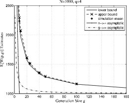
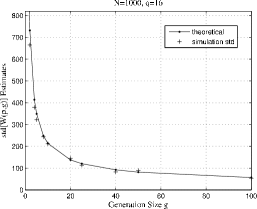
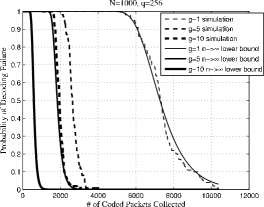
Figure 22 shows several estimates of $E[W(\boldsymbol{\rho},\mathbf{g})]$, and Figure 22 shows the standard deviation of $W(\boldsymbol{\rho},\mathbf{g})$ calculated from Theorem 8 and simulation results, when $\rho_{i}=\frac{1}{n}$ and $g_{i}=g$ for $i=1,2,\dots,n$. The estimates are plotted versus the uniform generation size $g$ for fixed $N=ng=1000.$

For coding over disjoint generations and a fixed total number of information packets, both the expected value and the standard deviation of the decoding latency drop significantly as the generation size $g$ grows to a relatively small value from the case where no coding is used ($g=1$). Hence, throughput is improved by a moderate increase in the computational cost that scales quadratically with the generation size (see Section II-E). On the other hand, we also observe that past a moderate generation size ($\sim 50-100$ coded packets for $N=1000$), the decrease in decoding latency becomes slower by further increasing the encoding/decoding complexity. We therefore argue for a “sweet spot” generation size which characterizes the tradeoff between throughput and complexity.

V-B Probability of Decoding Failure

In this subsection we assume uniform generation size and scheduling probability, i.e., $\rho_{i}=\frac{1}{n}$, $g_{i}=g$ for $i=1,2,\dots,n$. For short, we denote $W(\boldsymbol{\rho},\mathbf{g})$ as $W_{n}(g)$. From Theorem 7, we obtain the following lower bound to the probability of decoding failure as $n\rightarrow\infty$:

Theorem 9

When $n\rightarrow\infty$, the probability of decoding failure when $t$ coded packets have been collected is greater than $1-\exp\left[-\frac{1}{(g-1)!}n(\log n)^{g-1}\exp\left(-\frac{t}{n}\right)\right]+\mathcal{O}\left(\frac{\log\log n}{\log n}\right)$.

Proof:

The probability of decoding failure after acquiring $t$ coded packets equals $\textnormal{Prob}[W_{n}(g)>t]$. Since $W_{n}(g)\geq T_{n}(g)$,

$$\textnormal{Prob}[W_{n}(g)>t]\geq\,\textnormal{Prob}[T_{n}(g)>t]$$

$$=1-\!\textnormal{Prob}\left[Y_{n}(g)\leq\frac{t}{n}-\log n-(g-1)\log\log n\right].$$

The result in Theorem 9 follows directly from Theorem 7. ∎

Corollary 10

When $g$ is fixed and $n\rightarrow\infty$, in order to make the probability of decoding failure smaller than $\delta$, the number of coded packets collected has to be at least $E[T_{n}(g)]-n\log\log\frac{1}{1-\delta}$. If $\delta=\frac{1}{N^{c}}$ for some constant $c$, then the number of coded packets necessary for successful decoding has to be at least $E[T_{n}(g)]+cn\log(ng)$.

Theorem 4.2 in [5] also gives the number of coded packets needed to have the probability of decoding failure below $\delta=\frac{1}{N^{c}}$, but under the assumption that $\ln(N/\delta)=o(N/n)=o(g)$. In comparison, Corollary 10 treats the case where $g$ is constant.

Figure 22 shows the estimate of the probability of decoding failure versus $T$, the number of coded packets collected. As pointed out in Remark 1, for $m\geq 2$, the deviation of the CDF of $T_{n}(m)$ from the limit law for $n\rightarrow\infty$ depends on $m$ and is on the order of $\mathcal{O}({\frac{\log\log n}{\log n}})$ for $m\geq 2$, which is quite slow, partly explaining the deviation of the limit law curves from the simulation curves for $m=5$ and $m=10$ in Figure 22.

VI Coding Over Overlapping Generations

Even when generations are scheduled uniformly at random, there will be more coded packets accumulated in some of the generations than in others. The “slowest” generation is the bottleneck for file decoding. It is then advisable to design a mechanism that allows “faster” generations to help those lagging behind. In this section, we propose the random annex code, a new coding scheme in which generations share randomly chosen packets, as opposed to previously proposed “head-to-toe” overlapping scheme of [7].

We provide a heuristic analysis of the code throughput based on our results for the coupon collection model and an examination of the overlapping structure. Previous work on coding over overlapping generations, [6] and [7], lacks accurate performance analysis for information blocks of moderate finite lengths. On the other hand, the computational effort needed to carry out our analysis scales well with the length of information, and the performance predictions coincide with simulation data. In addition, we find that our random annex code outperforms the “head-to-toe” overlapping scheme of [7] over a unicast link.

In this section we conveniently assume that the coded packets are sent over a perfect channel, since here we are interested in comparing the performance of different rateless coding schemes.

VI-A Forming Overlapping Generations

We form $n$ overlapping generations out of a file with $N$ information packets in two steps as follows:

1. Partition the file set $\mathcal{F}$ of $N$ packets into subsets $B_{1},B_{2},\dots,B_{n}$, each containing $h$ consecutive packets. These $n=N/h$ subsets are referred to as base generations. Thus, $B_{i}=\{p_{(i-1)h+1},p_{(i-1)h+2},\dots,p_{ih}\}$ for $i=1,2,\dots,n$. $N$ is assumed to be a multiple of $h$ for convenience. In practice, if $N$ is not a multiple of $h$, set $n=\lceil N/h\rceil$ and assign the last $[N-(n-1)h]$ packets to the last (smaller) base generation.

2. To each base generation $B_{i}$, add a random annex $R_{i}$, consisting of $l$ packets chosen uniformly at random (without replacement) from the $N-h=(n-1)h$ packets in $\mathcal{F}\backslash B_{i}$. The base generation together with its annex constitutes the extended generation $G_{i}=B_{i}\cup R_{i}$, the size of which is $g=h+l$. Throughout this paper, unless otherwise stated, the term “generation” will refer to “extended generation” whenever used alone for overlapping generations.

The generation scheduling probabilities are chosen to be uniform, $\rho_{1}=\rho_{2}=\dots=\rho_{n}=1/n$. The encoding and decoding procedures run the same as described in the general model in Section II.

VI-B Analyzing the Overlapping Structure

The following Claims 11 through 14 present combinatorial derivations of quantities concerning the frequency at which an arbitrary information packet is represented in different generations.

Claim 11

For any packet in a base generation $B_{k}$, the probability that it belongs to annex $R_{r}$ for some $r\in\{1,2,\dots,n\}\backslash\{k\}$ is

$$\pi={{N-h-1}\choose{l-1}}/{{N-h}\choose{l}}=\frac{l}{N-h}=\frac{l}{(n-1)h},$$

whereas the probability that it does not belong to $R_{r}$ is $\bar{\pi}=1-\pi.$

Claim 12

Let $X$ be the random variable representing the number of generations an information packet participates in. Then, $X=1+Y,$ where $Y$ is ${\rm Binom}(n-1,\pi).$

$$E[X]=1+(n-1)\pi=1+\frac{l}{h},$$

and

$$Var[X]=(n-1)\pi\bar{\pi}.$$

Claim 13

In each generation of size $g=h+l$, the expected number of information packets not participating in any other generation is $h\bar{\pi}^{(n-1)}\approx he^{-l/h}$ for $n\gg 1$; the expected number of information packets participating in at least two generations is

$$l+h[1-\bar{\pi}^{(n-1)}]\approx l+h\left[1-e^{-l/h}\right]<\min\{g,2l\}$$

for $n\gg 1$ and $l>0$.

Claim 14

The probability that two generations overlap is $1-{{N-2h}\choose{l,l,N-2h-2l}}/{{N-h}\choose l}^{2}$. The number of generations overlapping with any one generation $G_{i}$ is then

$${\rm Binom}\left(n-1,\left[1-{{N-2h}\choose{l,l,N-2h-2l}}/{{N-h}\choose l}^{2}\right]\right).$$

The following Theorem 15 quantifies the expected amount of help a generation may receive from previously decoded generations in terms of common information packets. In the next subsection, we use Corollary 5 and Theorem 15 for a heuristic analysis of the expected throughput performance of the random annex code.

Theorem 15

For any $I\subset\{1,2,\dots,n\}$ with $|I|=s$, and any $j\in\{1,2,\dots,n\}\backslash I$,

$$\Omega(s)=E[|\left(\cup_{i\in I}G_{i}\right)\cap G_{j}|] =g\cdot\left[1-\bar{\pi}^{s}\right]+sh\cdot\pi\bar{\pi}^{s}$$ (19)

where $|B|$ denotes the cardinality of set $B$. When $n\rightarrow\infty$, if $\frac{l}{h}\rightarrow\alpha$ and $\frac{s}{n}\rightarrow\beta$, and let $\omega(\beta)=\Omega(s)$, then $\omega(\beta)\rightarrow h\left[(1+\alpha)\left(1-e^{-\alpha\beta}\right)+\alpha\beta e^{-\alpha\beta}\right]$.

Proof:

Please refer to Appendix D. ∎

VI-C Expected Throughput Analysis: The Algorithm

Given the overlapping structure, we next describe an analysis of the expected number of coded packets a receiver needs to collect in order to decode all $N$ information packets of $\mathcal{F}$ when they are encoded by the random annex code. We base our analysis on Theorem 15 above, Corollary 5 in Section IV, and also (3) in Section III, and use the mean value for every quantity involved.

By the time when $s$ $(s=0,1,\dots,n-1)$ generations have been decoded, for any one of the remaining $(n-s)$ generations, on the average $\Omega(s)$ of its participating information packets have been decoded, or equivalently, $(g-\Omega(s))$ of them are not yet resolved. If for any one of these remaining generations the receiver has collected enough coded packets to decode its unresolved packets, that generation becomes the $(s+1)$th decoded; otherwise, if no such generation exists, decoding fails.

The quantity $\eta_{g}(x)$ defined in (3) in Section III estimates the number of coded packets from a generation of size $g$ adequate for collecting $x$ linearly independent equations. By extending the domain of $\eta_{g}(x)$ from integers to real numbers, we can estimate that the number of coded packets needed for the $(s+1)$th decoded generation should exceed $m^{\prime}_{s}=\lceil\eta_{g}(g-\Omega(s))\rceil$. Since in the random annex code, all generations are randomly scheduled with equal probability, for successful decoding, we would like to have at least $m^{\prime}_{0}$ coded packets belonging to one of the generations, at least $m^{\prime}_{1}$ belonging to another, and so on. Then Corollary 5 in Section IV can be applied to estimate the total number of coded packets needed to achieve these minimum requirements for the numbers of coded packets.

The algorithm for our heuristic analysis is listed as follows:

1. Compute $\Omega(s-1)$ for $s=1,\dots,n$ using Theorem 15;

2. Compute $m_{s}^{\prime}=\lceil\eta_{g}(g-\Omega(s-1))\rceil$ for $s=1,2,\dots,n$ using (3);

3. Map $m_{s}^{\prime}$ $(s=1,2,\dots,n)$ into $A$ values $m_{j}$ $(j=1,2,\dots,A)$ so that $m_{j}=m_{k_{j-1}+1}^{\prime}=m_{k_{j-1}+2}^{\prime}=\dots=m_{k_{j}}^{\prime}$, for $j=1,2,\dots,A$, $k_{0}=0$ and $k_{A}=n$;

4. Evaluate (10) in Corollary 5 with the $A$, $k_{j}$s, and $m_{j}$s obtained in Step 3), as an estimate for the expected number of coded packets needed for successful decoding.

Remark 2

The above Step 3) is viable because $\Omega(s)$ is nondecreasing in $s$, $\eta_{g}(x)$ is non-decreasing in $x$ for fixed $g$, and thus $m_{s}^{\prime}$ is non-increasing in $s$.

Although our analysis is heuristic, we will see in the next section that the estimate closely follows the simulated average performance curve of the random annex coding scheme.

VI-D Numerical Evaluation and Simulation Results

VI-D1 Throughput vs. Complexity in Fixed Number of Generations Schemes

Our goal here is to find out how the annex size $l$ affects the decoding latency of the scheme with fixed base generation size $h$ and the total number of information packets $N$ (and consequently, the number of generations $n$). Note that the generation size $g=h+l$ affects the computational complexity of the scheme, and hence we are actually looking at the tradeoff between throughput and complexity.

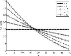
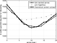
Figure 3 shows both the analytical and simulation results when the total number $N$ of information packets is $1000$ and the base generation size $h$ is $25$. Figure 33 shows $h+l-\Omega(s)$ for $s=0,1,\dots,n$ with different annex sizes. Recall that $\Omega(s)$ is the expected size of the overlap of the union of $s$ generations with any one of the leftover $n-s$ generations. After the decoding of $s$ generations, for any generation not yet decoded, the expected number of information packets that still need to be resolved is then $h+l-\Omega(s)$. We observe that the $h+l-\Omega(s)$ curves start from $h+l$ for $s=0$ and gradually descends, ending somewhere above $h-l$, for $s=n-1$.

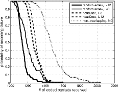
Recall that we measure throughput by decoding latency (Section II-F). Figure 33 shows the expected performance of the random annex code, along with the performance of the head-to-toe overlapping code and the non-overlapping code ($l=0$). Figure 33 shows the probability of decoding failure of these codes versus the number of coded packets collected.

Figure 3: $N=1000$, $h=25$, $q=256$: 3 Difference between the generation size and the expected size of overlap with previously decoded generations $(h+l-\Omega(s))$; 3 Expected number of coded packets needed for successful decoding versus annex size $l$; 3 Probability of decoding failure

• Our analysis for the expected decoding latency closely matches the simulation results.

• Figure 33 shows that by fixing the file size $N$ and the base generation size $h$, the expected decoding latency decreases roughly linearly with increasing annex size $l$, up to $l=12$ for the random annex scheme and up to $l=8$ for the head-to-toe scheme. Meanwhile, the decoding cost per information packet is quadratic in $g=h+l$. Beyond the optimal annex size, throughput cannot be further increased by raising computational cost.

• The random annex code outperforms head-to-toe overlapping at their respective optimal points. Both codes outperform the non-overlapping scheme.

• As more coded packets are collected, the probability of decoding failure of the random annex code converges to $0$ faster than that of the head-to-toe and that of the non-overlapping scheme.

Overlaps provide a tradeoff between computational complexity and decoding latency.

VI-D2 Enhancing Throughput in Fixed Complexity Schemes

Our goal here is to see if we can choose the annex size to optimize the throughput with negligible sacrifice in complexity. To this end, we fix the extended generation size $g=h+l$ and vary only the annex size $l$. Consequently, the computational complexity for coding does not increase when $l$ increases. Actually, since some of the information packets in a generation of size $g$ could already be solved while decoding other generations, the remaining information packets in this generation can be solved in a system of linear equations of fewer than $g$ unknowns, and as a result increasing $l$ might decrease the decoding complexity.

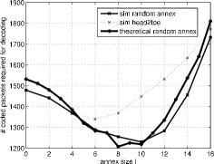
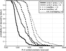
Figure 4 shows both the analytical and simulation results for the code performance when the total number $N$ of information packets is fixed at $1000$ and size $g$ of extended generation fixed at $25$.

Figure 4: $N=1000$, $g=h+l=25$, $q=256$: 4 Expected number of coded packets needed for successful decoding versus annex size $l$; 4 Probability of decoding failure

• Again our analytical results agree with simulation results very well;

• It is interesting to observe that, without raising computational complexity, increasing annex size properly can still give non-negligible improvement to throughput;

• Figure 44 shows a roughly linear improvement of throughput with increasing $l$, up to $l=10$ for the random annex scheme and up to $l=6$ for the head-to-toe scheme. Increasing $l$ beyond affects throughput adversely;

• The random annex code again outperforms head-to-toe overlapping at their optimal points. Both codes outperform the non-overlapping scheme;

• We again observe that the probability of decoding failure of the random annex code converges faster than those of the head-to-toe and the non-overlapping schemes.

When the overlap size increases, we either have larger generations with unchanged number of generations, or a larger number of generations with unchanged generation size. In both cases the decoding latency would increase if we neglected the effect of overlaps during the decoding process. If we make use of the overlap in decoding, on the other hand, the larger the overlap size, the more help the generations can lend to each other in decoding and, hence, reducing the decoding latency. Two canceling effects result in a non-monotonic relationship between throughput and overlap size.

Figure 5: Optimal expected decoding latency and the optimal overlap size with random annex codes. $N=1000$, $q=16$

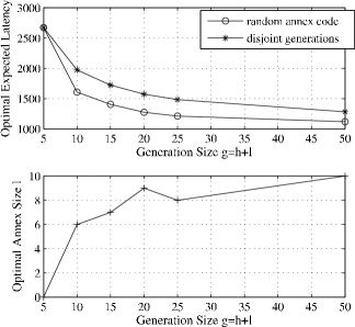
The effect of generation size on the throughput of random annex codes is further illustrated in Figure 5. Figure 5 plots the optimal expected decoding latency achievable by random annex codes and the corresponding optimal annex size versus the generation size for $N=1000$ and $q=16.$ The plotted values are calculated using the algorithm listed in Section VI-C. We can see from Figure 5 that with the random annex code and a generation size of $20$, the expected throughput is better than what can be achieved with coding over disjoint generations and a generation size of $50$. The reduction in computational complexity is considerable. Capturing the optimal overlap size in terms of other parameters of the code is our object of interest in the future.

Appendix A Proof of Claim 1

For $i=1,2,\dots,n$ and any $s\geq g$, we have

$$\ln\textnormal{Prob} \bigl{\{}M(g,g)\leq s\bigr{\}}$$

$$= \ln\prod_{k=0}^{h-1}(1-q^{k-s})=\sum_{k=0}^{g-1}\ln(1-q^{k-s})$$

$$= -\sum_{k=0}^{g-1}\sum_{j=1}^{\infty}\frac{1}{j}q^{(k-s)j}=-\sum_{j=1}^{\infty}\frac{1}{j}\sum_{k=0}^{g-1}q^{j(k-s)}$$

$$= -\sum_{j=1}^{\infty}\frac{1}{j}q^{-js}\frac{q^{jg}-1}{q^{j}-1}$$

$$= -q^{-(s-g)}\sum_{j=1}^{\infty}\frac{1}{j}q^{-(j-1)(s-g)}\frac{1-q^{-jg}}{q^{j}-1}$$

$$> q^{-(s-g)}\sum_{j=1}^{\infty}\frac{1}{j}\frac{1-q^{-jg}}{1-q^{j}}$$

$$= q^{-(s-g)}\ln\textnormal{Prob}\bigl{\{}M(g,g)\leq g\bigr{\}}$$

$$> q^{-(s-g)}\lim_{h\rightarrow\infty,q=2}\ln\textnormal{Prob}\bigl{\{}M(g,g)\leq g\bigr{\}}$$

The claim is obtained by setting

$$\alpha_{q,g}=-\ln\textnormal{Prob}\bigl{\{}M(g,g)\leq g\bigr{\}},\;$$

and

$$\alpha_{2,\infty}=-\!\!\lim_{g\rightarrow\infty,q=2}\ln\textnormal{Prob}\bigl{\{}M(g,g)\leq g\bigr{\}}.$$

Appendix B Proofs of Generalized Results of Collector’s Brotherhood Problem

Proof of Theorem 2

Our proof generalizes the symbolic method of [10].

Let $\xi$ be the event that the number of copies of coupon $G_{i}$ is at least $m_{i}$ for every $i=1,2,\dots,n$. For integer $t\geq 0$, let $\xi(t)$ be the event that $\xi$ has occurred after a total of $t$ samplings, and let $\bar{\xi}(t)$ be the complementary event. Then, the tail probability $\mathrm{Prob}[T(\boldsymbol{\rho},\mathbf{m})>t]=\mathrm{Prob}[\bar{\xi}(t)]=\nu_{t}$.

To derive $\nu_{t}$, we introduce an operator $f$ acting on an $n$-variable polynomial $g$. $f$ removes all monomials $x_{1}^{w_{1}}x_{2}^{w_{2}}\dots x_{n}^{w_{n}}$ in $g$ satisfying $w_{1}\geq m_{1},\dots,w_{n}\geq m_{n}$. Note that $f$ is a linear operator, i.e., if $g_{1}$ and $g_{2}$ are two polynomials in the same $n$ variables, and $a$ and $b$ two scalars, we have $af(g_{1})+bf(g_{2})=f(ag_{1}+bg_{2})$.

Each monomial in $(x_{1}+\dots+x_{n})^{t}$ corresponds to one of the $n^{t}$ possible outcomes of $t$ samplings, with the exponent of $x_{i}$ being the number of copies of coupon $G_{i}$. Since the samplings are independent, the probability of an outcome $x_{1}^{w_{1}}x_{2}^{w_{2}}\dots x_{n}^{w_{n}}$ is $\rho_{1}^{w_{1}}\rho_{2}^{w_{2}}\dots\rho_{n}^{w_{n}}$. Hence, the probability of $\bar{\xi}(t)$ is $f((x_{1}+\dots+x_{n})^{t})$, when evaluated at $x_{i}=\rho_{i}$ for $i=1,2,\dots n$, i.e.,

$$\nu_{t}=f((x_{1}+\dots+x_{n})^{t})|_{x_{i}=\rho_{i},i=1,\dots,n}.$$ (20)

Hence, (20) and (7) lead to

$$\varphi_{T(\boldsymbol{\rho},\mathbf{m})}(z)=\sum_{t\geq 0}f\left((x_{1}+\dots+x_{n})^{t}\right)z^{t}|_{x_{i}=\rho_{i},i=1,\dots,n}.$$

The identity

$$\int_{0}^{\infty}\frac{1}{t!}y^{t}e^{-y}dy=1$$

and the linearity of the operator $f$ imply that

$$\varphi_{T(\boldsymbol{\rho},\mathbf{m})}(z)= \int_{0}^{\infty}\sum_{t\geq 0}\frac{f\left((x_{1}+\dots+x_{n})^{t}\right)}{t!}z^{t}y^{t}e^{-y}dy$$

$$= \int_{0}^{\infty}f\Bigl{(}\sum_{t\geq 0}\frac{(x_{1}zy+\dots+x_{n}zy)^{t}}{t!}\Bigr{)}e^{-y}dy$$

$$= \int_{0}^{\infty}f\left(\exp(x_{1}zy+\dots+x_{n}zy)\right)e^{-y}dy$$ (21)

evaluated at $x_{i}=\rho_{i},i=1,\dots,n$.

We next find the sum of the monomials in the polynomial expansion of $\exp(x_{1}+\dots+x_{n})$ that should be removed under $f$. Clearly, this sum should be $\prod_{i=1}^{n}\left(e^{x_{i}}-S_{m_{i}}(x_{i})\right)$, where $S$ is defined in (5) and (6)). Therefore,

$$f\left(\exp(x_{1}zy+\dots+x_{n}zy)\right)|_{x_{i}=\rho_{i},i=1,\dots,n}$$

$$=e^{zy}-\prod_{i=1}^{n}\left(e^{\rho_{i}zy}-S_{m_{i}}(\rho_{i}zy)\right).$$

$$\varphi_{T(\boldsymbol{\rho},\mathbf{m})}(z)= \int_{0}^{\infty}\left[e^{zy}-\prod_{i=1}^{n}\left(e^{\rho_{i}zy}-S_{m_{i}}(\rho_{i}zy)\right)\right]e^{-y}dy$$ (22)

Proof of Corollary 3

Note that

$$\varphi_{T(\boldsymbol{\rho},\mathbf{m})}(z) =\sum_{t=0}^{\infty}\mathrm{Prob}[T(\boldsymbol{\rho},\mathbf{m})>t]z^{t}$$

$$=\sum_{t=0}^{\infty}\sum_{j=t+1}^{\infty}\mathrm{Prob}[T(\boldsymbol{\rho},\mathbf{m})=j]z^{t}$$

$$=\sum_{j=1}^{\infty}\mathrm{Prob}[T(\boldsymbol{\rho},\mathbf{m})=j]\sum_{t=0}^{j-1}z^{t}$$

$$E[T(\boldsymbol{\rho},\mathbf{m})] =\sum_{j=1}^{\infty}j\mathrm{Prob}[T(\boldsymbol{\rho},\mathbf{m})=j]=\varphi_{T(\boldsymbol{\rho},\mathbf{m})}(1).$$

Similarly,

$$\varphi_{T(\boldsymbol{\rho},\mathbf{m})}^{\prime}(z) =\sum_{t=0}^{\infty}t\mathrm{Prob}[T(\boldsymbol{\rho},\mathbf{m})>t]z^{t-1}$$

$$=\sum_{j=1}^{\infty}\mathrm{Prob}[T(\boldsymbol{\rho},\mathbf{m})=j]\sum_{t=0}^{j-1}tz^{t-1}$$

$$\varphi_{T(\boldsymbol{\rho},\mathbf{m})}^{\prime}(1) =\sum_{j=1}^{\infty}\frac{1}{2}j(j-1)\mathrm{Prob}[T(\boldsymbol{\rho},\mathbf{m})=j].$$

Hence,

$$E[T(\boldsymbol{\rho},\mathbf{m})^{2}]= \sum_{j=1}^{\infty}j^{2}\mathrm{Prob}[T(\boldsymbol{\rho},\mathbf{m})=j]$$

$$= 2\varphi_{T(\boldsymbol{\rho},\mathbf{m})}^{\prime}(1)+\varphi_{T(\boldsymbol{\rho},\mathbf{m})}(1),$$

and consequently,

$$\text{Var}[T(\boldsymbol{\rho},\mathbf{m})]=2\varphi_{T(\boldsymbol{\rho},\mathbf{m})}^{\prime}(1)+\varphi_{T(\boldsymbol{\rho},\mathbf{m})}(1)-\varphi_{T(\boldsymbol{\rho},\mathbf{m})}^{2}(1).$$

We have

$$\varphi_{T(\boldsymbol{\rho},\mathbf{m})}^{\prime}(z)=$$

$$\int_{0}^{\infty}x\biggl{(}e^{-x(1-z)}-\sum_{i=1}^{n}\rho_{i}\frac{e^{-\rho_{i}x(1-z)}-S_{m_{i}-1}(\rho_{i}xz)e^{-\rho_{i}x}}{e^{-\rho_{i}x(1-z)}-S_{m_{i}}(\rho_{i}xz)e^{-\rho_{i}x}}\cdot$$

$$\quad\cdot\prod_{j=1}^{n}\left(e^{-\rho_{j}x(1-z)}-S_{m_{j}}(\rho_{j}xz)e^{-\rho_{j}x}\right)\biggr{)}dx,$$

and from there, we can get $\varphi_{T(\boldsymbol{\rho},\mathbf{m})}^{\prime}(1)$ and $\text{Var}[T(\boldsymbol{\rho},\mathbf{m})].$

Proof of Theorem 4

We again apply the Newman-Shepp symbolic method. Similar to the proof of Theorem 2, we introduce an operator $f$ acting on an $n$-variable polynomial $g$. For a monomial $x_{1}^{w_{1}}\dots x_{n}^{w_{n}}$, let $i_{j}$ be the number of exponents $w_{u}$ among $w_{1},\dots,w_{n}$ satisfying $w_{u}\geq k_{j}$, for $j=1,\dots,A$. $f$ removes all monomials $x_{1}^{w_{1}}\dots x_{n}^{w_{n}}$ in $g$ satisfying $i_{1}\geq k_{1},\dots,i_{A}\geq k_{A}$ and $i_{1}\leq\dots\leq i_{A}$. $f$ is again a linear operator. One can see that

$$\varphi_{U(\mathbf{m},\mathbf{k})}(z)=$$ (23)

$$\int_{0}^{\infty}f\left(\exp(x_{1}zy+\dots+x_{n}zy)\right)e^{-y}dy|_{x_{1}=x_{2}=\dots=x_{n}=\frac{1}{n}}.$$

We choose integers $0=i_{0}\leq i_{1}\leq\dots\leq i_{A}\leq i_{A+1}=n$, such that $i_{j}\geq k_{j}$ for $j=1,\dots,A$, and then partition indices $\{1,\dots,n\}$ into $(A+1)$ subsets $\mathcal{I}_{1},\dots,\mathcal{I}_{A+1}$, where $\mathcal{I}_{j}(j=1,\dots,A+1)$ has $i_{j}-i_{j-1}$ elements. Then

$$\prod_{j=1}^{A+1}\prod_{i\in\mathcal{I}_{j}}(S_{m_{j-1}}(x_{i})-S_{m_{j}}(x_{i}))$$ (24)

equals the sum of all monomials in $\exp(x_{1}+\dots+x_{n})$ with ($i_{j}-i_{j-1}$) of the $n$ exponents smaller than $m_{j-1}$ but greater than or equal to $m_{j}$, for $j=1,\dots,A+1$. (Here $S$ is as defined by (5-6).) The number of such partitions of $\{1,\dots,n\}$ is equal to ${{n}\choose{n-i_{A},\dots,i_{2}-i_{1},i_{1}}}=\prod_{j=0}^{A}{{i_{j+1}}\choose{i_{j}}}$. Finally, we need to sum the terms of the form (24) over all partitions of all choices of $i_{1},\dots,i_{A}$ satisfying $k_{j}\leq i_{j}\leq i_{j+1}$ for $j=1,\dots,A$:

$$f\left(\exp(x_{1}zy+\dots+x_{n}zy)\right)|_{x_{1}=\dots=x_{n}=\frac{1}{n}}=\exp(zy)-$$

$$\sum_{{{(i_{0},i_{1},\dots,i_{A+1}):\atop i_{0}=0,i_{A+1}=n}\atop i_{j}\in[k_{j},i_{j+1}]}\atop j=1,2,\dots,A}\prod_{j=0}^{A}{{i_{j+1}}\choose{i_{j}}}\left[S_{m_{j}}(\frac{zy}{n})-S_{m_{j+1}}(\frac{zy}{n})\right]^{i_{j+1}-i_{j}}.$$ (25)

Bringing (B) into (23) gives our result in Theorem 4.

Appendix C Proof of Theorem 8

$$E[ W(\boldsymbol{\rho},\mathbf{g})]$$

$$=\sum_{\mathbf{m}}\left(\prod_{i=1}^{n}\textnormal{Pr}[M_{i}=m_{i}]\right)E[T(\boldsymbol{\rho},\mathbf{m})]$$

$$=\int_{0}^{\infty}\left[1-\prod_{i=1}^{n}\sum_{m_{i}}\textnormal{Pr}[M_{i}=m_{i}](1-S_{m_{i}}(\rho_{i}x)e^{-\rho_{i}x})\right]dx$$ (26)

$$=\int_{0}^{\infty}\left(1-\prod_{i=1}^{n}\left(1-e^{-\rho_{i}x}E_{M_{i}}\left[S_{M_{i}}(\rho_{i}x)\right]\right)\right)dx.$$

(26) comes from the distributivity.

Since

$$E_{M_{i}}\left[S_{M_{i}}(\rho_{i}x)\right]=\sum_{j=0}^{\infty}\frac{(\rho_{i}x)^{j}}{j!}\textnormal{Pr}[M_{i}>j],$$

by Claim 1,

$$E_{M_{i}}\left[S_{M_{i}}(\rho_{i}x)\right]$$

$$<S_{g_{i}}(\rho_{i}x)+\sum_{j=g_{i}}^{\infty}\frac{(\rho_{i}x)^{j}}{j!}\alpha_{q,g}q^{-(j-g)}$$

$$=S_{g_{i}}(\rho_{i}x)+\alpha_{q,g_{i}}q^{g_{i}}e^{\rho_{i}x/q}-\alpha_{q,g_{i}}q^{g_{i}}S_{g_{i}}(\rho_{i}x/q),$$

where

$$\alpha_{q,g_{i}}=-\ln\textnormal{Pr}\bigl{\{}M(g_{i},g_{i})\leq g_{i}\bigr{\}}=-\sum_{k=0}^{g_{i}-1}\ln\left(1-q^{k-g_{i}}\right)$$

for $i=1,2,\dots,n$.

Hence, we have (17).

Expression (18) for $E[W^{2}(\boldsymbol{\rho},\mathbf{g})]$ can be derived in the same manner, and then the expression for $\text{Var}[W(\boldsymbol{\rho},\mathbf{g})]$ immediately follows.

Appendix D Proof of Theorem 15

Without loss of generality, let $I=\{1,2,\dots,s\}$ and $j=s+1$, and define $\mathcal{R}_{s}=\cup_{i=1}^{s}R_{i}$, $\mathcal{B}_{s}=\cup_{i=1}^{s}B_{i}$, and $\mathcal{G}_{s}=\cup_{i=1}^{s}G_{i}$ for $s=0,1,\dots,n-1$. Then, $E\left[|\left(\cup_{i\in I}G_{i}\right)\cap G_{j}|\right]=E\left[|\mathcal{G}_{s}\cap G_{s+1}|\right]$. For any two sets $X$ and $Y$, we use $X+Y$ to denote $X\cup Y$ when $X\cap Y=\emptyset$.

$$\mathcal{G}_{s}\cap G_{s+1}= (\mathcal{B}_{s}+\mathcal{R}_{s}\backslash\mathcal{B}_{s})\cap(B_{s+1}+R_{s+1})$$

$$= \mathcal{B}_{s}\cap R_{s+1}+\mathcal{R}_{s}\cap B_{s+1}+(\mathcal{R}_{s}\backslash\mathcal{B}_{s})\cap R_{s+1},$$

and therefore

$$E[|\mathcal{G}_{s}\cap G_{s+1}|]= E[|\mathcal{B}_{s}\cap R_{s+1}|]+$$ (27)

$$E[|\mathcal{R}_{s}\cap B_{s+1}|]+E[|(\mathcal{R}_{s}\backslash\mathcal{B}_{s})\cap R_{s+1}|].$$

Using Claim 11, we have

$$E[|\mathcal{B}_{s}\cap R_{s+1}|]=sh\pi,$$ (28)

$$E[|\mathcal{R}_{s}\cap B_{s+1}|]=h[1-(1-\pi)^{s}],$$ (29)

$$E[|(\mathcal{R}_{s}\backslash\mathcal{B}_{s})\cap R_{s+1}|]=(n-s-1)h\pi[1-(1-\pi)^{s}],$$ (30)

where $\pi$ is as defined in Claim 11. Bringing (28)-(30) into (27), we obtain (19).

Furthermore, when $n\rightarrow\infty$, if $l/h\rightarrow\alpha$ and $s/n\rightarrow\beta$, then

$$E[|\mathcal{G}_{s}\cap G_{s+1}|]= g\cdot\left[1-\bar{\pi}^{s}\right]+sh\cdot\pi\bar{\pi}^{s}$$

$$\rightarrow h(1+\alpha)\Bigl{[}1-\Bigl{(}1-\frac{\alpha}{n-1}\Bigr{)}^{n\beta}\Bigr{]}+$$

$$h\alpha\beta\Bigl{(}1-\frac{\alpha}{n-1}\Bigr{)}^{n\beta}$$

$$\rightarrow h\Bigl{[}(1+\alpha)(1-e^{-\alpha\beta})+\alpha\beta e^{-\alpha\beta}\Bigr{]}$$

$$= h\Bigl{[}1+\alpha-(1+\alpha-\alpha\beta)e^{-\alpha\beta}\Bigr{]}$$

References

- [1] T. Ho, R. Koetter, M. Medard, D. Karger, and M. Effros, “The benefits of coding over routing in a randomized setting,” in Proc. IEEE International Symposium on Information Theory (ISIT’03), 2003, p. 442.
- [2] C. Gkantsidis and P. Rodriguez, “Network coding for large scale content distribution,” in Proc. the 24th Annual Joint Conference of the IEEE Computer and Communications Societies (INFOCOM’05), vol. 4, Miami, FL, Mar. 2005, pp. 2235–2245.
- [3] Z. Liu, C. Wu, B. Li, and S. Zhao, “UUSee: Large-scale operational on-demand streaming with random network coding,” in Proc. the 30th IEEE Conference on Computer Communications (INFOCOM’10), San Diego, California, Mar. 2010.
- [4] P. A. Chou, Y. Wu, and K. Jain, “Practical network coding,” in Proc. 41st Annual Allerton Conference on Communication, Control, and Computing, Monticello, IL, Oct. 2003.
- [5] P. Maymounkov, N. Harvey, and D. S. Lun, “Methods for efficient network coding,” in Proc. 44th Annual Allerton Conference on Communication, Control, and Computing, Monticello, IL, Sept. 2006.
- [6] D. Silva, W. Zeng, and F. Kschischang, “Sparse network coding with overlapping classes,” in Proc. Workshop on Network Coding, Theory, and Applications (NetCod ’09), Lausanne, Switzerland, Jun. 2009, pp. 74–79.
- [7] A. Heidarzadeh and A. Banihashemi, “Overlapped chunked network coding,” in IEEE Information Theory Workshop (ITW’10), Jan. 2010, pp. 1–5.
- [8] W. Feller, An Introduction to Probability Theory and Its Applications, 3rd ed. New York: John Wiley & Sons Inc., 1968, vol. 1, pp. 224–225.
- [9] C. Fragouli and E. Soljanin, Network Coding Applications, ser. Foundations and Trends in Networking. Hanover, MA: now Publishers Inc., Jan. 2008, vol. 2, no. 2, pp. 146–147.
- [10] D. Newman and L. Shepp, “The double dixie cup problem,” The American Mathematical Monthly, vol. 67, no. 1, pp. 58–61, Jan. 1960.
- [11] D. Foata and D. Zeilberger, “The collector’s brotherhood problem using the Newman-Shepp symbolic method,” Algebra Universalis, vol. 49, no. 4, pp. 387–395, 2003.
- [12] A. Boneh and M. Hofri, “The coupon-collector problem revisited – a survey of engineering problems and computational methods,” Stochastic Models, vol. 13, pp. 39 – 66, 1997. [Online]. Available: http://www.informaworld.com/10.1080/15326349708807412
- [13] P. Flajolet, D. Gardy, and L. Thimonier, “Birthday paradox, coupon collectors, caching algorithms and self-organizing search,” Discrete Applied Mathematics, vol. 39, no. 3, pp. 207–229, 1992.
- [14] L. Flatto, “Limit theorems for some random variables associated with urn models,” The Annals of Probability, vol. 10, no. 4, pp. 927–934, 1982. [Online]. Available: http://www.jstor.org/stable/2243548
- [15] A. N. Myers and H. S. Wilf, “Some new aspects of the coupon collector’s problem,” SIAM Rev., vol. 48, no. 3, pp. 549–565, 2006.
- [16] P. Erdös and A. Rényi, “On a classical problem of probability theory,” Magyar Tud. Akad. Mat. Kutató Int. Közl., vol. 6, pp. 215–220, 1961.