Mass-Transport Models with Multiple-Chipping Processes

Abstract

We study mass-transport models with multiple-chipping processes. The rates of these processes are dependent on the chip size and mass of the fragmenting site. In this context, we consider $k$-chip moves (where $k$ $=$ $1,2,3,....$); and combinations of $1$-chip, $2$-chip and $3$-chip moves. The corresponding mean-field (MF) equations are solved to obtain the steady-state probability distributions, $P(m)$ vs. $m$. We also undertake Monte Carlo (MC) simulations of these models. The MC results are in excellent agreement with the corresponding MF results, demonstrating that MF theory is exact for these models.

I Introduction

The formation of structures at the nanoscale has attracted a lot of attention lagally ; z&l . The morphological and statistical properties of these systems are governed by microscopic processes like adsorption and desorption, fragmentation, diffusion and aggregation, etc. Different non-equilibrium steady-states can be accessed and phase transitions induced if the rates of the these processes are varied. Several experimental and theoretical studies have focused on adatom and cluster diffusion venables ; bartelt ; bales ; kuipers ; takayasu1 ; takayasu2 ; sk1 . However, there are relatively few studies which consider the fragmentation of clusters, expected to commonly occur during hyperthermal ion beam depositions and sputter depositions rusanen ; blandin1 ; blandin2 ; roder . The bombardment of clusters by energetic ions induces large island boundary fluctuations which cause multiple-chipping events rusanen ; wucher . These systems have received limited attention to date because of the unavailability of experimental probes to observe fragmentation. Further, the occurrence of these events is often on a pico-second time scale, making collection of data difficult.

The processes of fragmentation and aggregation significantly affect the growth mechanism by altering the number of small and large clusters. The steady-state cluster-size distribution in these systems is generally characterized by an exponentially decaying tail rusanen ; gpsup . In contrast, systems with adatom and cluster diffusion exhibit steady-state distributions which are power laws takayasu1 ; sk1 ; kuiri .

In many physical systems, the fragmentation kernel depends upon the masses of the chip size and the fragmenting cluster. For example, recent experiments on $Au$ clusters sputtered from embedded $Au$ nanoparticles report distinct chipping kernels for small and large clusters kuiri . In a related context, groups, herds, schools and flocks of animals also exhibit size-dependent fragmentation bonabeau1 ; bonabeau2 . Similar observations have been made in the context of polymerization ziff , gelation ziff and complex networks kwon . In all these systems, the steady-state distributions are either exponentials or power laws or their combinations.

Fragmentation is thus a ubiquitous phenomenon, observed in a variety of physical systems. In the present paper, we study conserved mass models with mass-dependent chipping – the fragmentation rates depend on the chip size and mass of the fragmenting site. We obtain the steady-state mass distributions of these models in the mean-field (MF) limit, and compare them with results from Monte Carlo (MC) simulations. The purpose of our study is to clarify the generic features of steady-state distributions in the presence of multiple-chipping processes.

This paper is organized as follows. In Section 2, we study models with mass-dependent fragmentation and aggregation processes. We focus on models with $k$-chip moves (where $k$ $=$ $1,2,3,...$); and combinations of $1$-chip, $2$-chip and $3$-chip moves. In Section 3, we present MC results for these models, and compare them with the corresponding MF solutions. We conclude this paper with a summary and discussion in Section 4.

II Transport Models with Mass-Dependent Chipping

Consider a mass-transport model on a discrete lattice where there is no adsorption or desorption. To begin with, masses $m_{i}(0)=0,1,2,$ etc. are placed randomly at each site $i$ with an overall mass density $\rho$. The evolution of the system is defined by the fragmentation kernel $g_{m}(n)$, i.e., the rate for a mass $n$ ($\leqslant m$) to chip from a site with mass $m$. The $n$-chip then deposits on a randomly-chosen nearest neighbor. The mass of the neighbor adds up, while that of the departure site decreases, with the total mass of the system remaining conserved. Typically, the steady-state mass distribution [$P(m)$] of sites with mass $m$ in these models shows either exponential or power-law decay with $m$.

We study the above model within a MF approximation which keeps track of the distribution of masses, ignoring correlations in the occupancy of adjacent sites. Although the MF theory suffers from this deficiency, our MC simulations in Sec. 3 show that it gives an accurate description of the above model, even in the 1-dimensional case. Let $P(m,t)$ denote the probability that a site has mass $m$ at time $t$. In the MF limit, $P(m,t)$ evolves as follows:

$$\frac{d}{dt}P(m,t) = -P(m,t)\sum_{m_{1}=1}^{m}g_{m}(m_{1})-P(m,t)\sum_{m_{2}=1}^{\infty}P(m_{2},t)\sum_{m_{1}=1}^{m_{2}}g_{m_{2}}(m_{1})$$ (1)

$$+\sum_{m_{1}=1}^{\infty}P(m+m_{1},t)g_{m+m_{1}}(m_{1})$$

$$+\sum_{m_{1}=1}^{m}P(m-m_{1},t)\sum_{m_{2}=m_{1}}^{\infty}P(m_{2},t)g_{m_{2}}(m_{1}),\ \ \ m\geq 1,$$

$$\frac{d}{dt}P(0,t) = -P(0,t)\sum_{m_{2}=1}^{\infty}P(m_{2},t){\sum_{m_{1}=1}^{m_{2}}}g_{m_{2}}(m_{1})+\sum_{m_{1}=1}^{\infty}P(m_{1},t)g_{m_{1}}(m_{1}).$$ (2)

Equations (1)-(2) enumerate all possible ways in which a site with mass $m$ may change its mass. The first term on the right-hand-side (RHS) of Eq. (1) is the “loss” due to chipping, while the second term represents the loss due to transfer of mass from a neighbor chipping. The third and fourth terms are the “gain” terms which represent the ways in which a site with mass greater (lesser) than $m$ can lose (gain) the excess (deficit) to yield mass $m$. The terms of Eq. (2) can be interpreted similarly. The above equations satisfy the sum rule

$$\frac{d}{dt}\sum_{m=0}^{\infty}P(m,t)=0,\quad\mbox{or}\quad\sum_{m=0}^{\infty}P(m,t)=1,$$ (3)

as required.

Next we consider a specific form of the mass-dependent chipping kernel, $g_{m}(n)=D(m)n^{-\alpha}$, where $\alpha\geqslant 0$ is a parameter. This kernel allows for chips of all sizes, with small masses being more likely to fragment from a site than large masses. It is especially relevant in the context of fragmentation of sputtered clusters. As revealed by Auger and thermal-desorption spectroscopy measurements performed on these nanostructures, fragments of a few atoms display a large mobility on the surface which rapidly decreases with increasing cluster size blandin1 ; davies .

Multiple-chip models may be interpreted as limiting cases of the above model. For $\alpha=\infty,$ this kernel only gives rise to $1$-chip processes. For large values of $\alpha$, we expect the fragmentation to be dominated by $1$-chip and $2$-chip processes with different rates. As the value of $\alpha$ is reduced, the possibility of higher-chip processes becomes appreciable. Finally, in the limit $\alpha=0,$ chips of any size are equally likely. Subsequently, we study $1$-chip models, ($1+2$)-chip models, etc. as approximations to the model with $g_{m}(n)=D(m)n^{-\alpha}$. It should be noted that the $n^{-\alpha}$-chipping kernel, unlike the multiple-chip models, includes the diffusion move, i.e., the movement of the entire mass $m$ at a site. The steady-state distribution for this model will be discussed in Section III.

II.1 $k$-chip models and the case $g_{m}(n)=g(n)$

First, we study $k$-chip models which act as building blocks to understand models in which chips of different sizes are allowed. The chipping kernel has the form

$$g_{m}(n)=w\delta_{n,k}.$$ (4)

The corresponding rate equations for $P(m,t)$, obtained by substituting Eq. (4) in Eqs. (1)-(2), are as follows (absorbing $w$ into the time $t$):

$$\frac{d}{dt}P(m,t) = -(1+s_{k})P(m,t)+P(m+k,t)+s_{k}P(m-k,t),\>m\geq k,$$ (5)

$$\frac{d}{dt}P(m,t) = -s_{k}P(m,t)+P(m+k,t),\quad m<k.$$ (6)

Here, $s_{k}(t)$ = $\sum_{m=k}^{\infty}P(m,t)$ is the probability of sites having mass $k$ or more.

In order to obtain the steady-state solution $P(m)$, the generating function $Q(z,t)$ $=$ $\sum_{m=1}^{\infty}z^{m}P(m,t)$ is computed from the above equations, and $\partial Q/\partial t$ is set to 0 in the steady state. $P(m)$ is then obtained by evaluating the integral

$$P(m) = \frac{1}{2\pi i}\int_{C}dz~{}\frac{Q(z)}{z^{m+1}},\hskip 8.5359ptm>1,$$ (7)

where the contour $C$ encircles the origin in the complex plane. The steady-state generating function of the $k$-chip model is

$$Q(z)=\frac{z(s_{1}-s_{2})+z^{2}(s_{2}-s_{3})+\cdot\cdot\cdot\cdot+z^{k}s_{k}(1-s_{1})}{(1-s_{k}z^{k})}.$$ (8)

The conservation of mass requires that $\sum_{m=1}^{\infty}mP(m)$ = $\rho$, where $\rho$ is the mass density. Putting $dQ/dz\big{|}_{z=1}=\rho$, we obtain

$$\rho=\frac{s_{1}+s_{2}+.......+s_{k}}{1-s_{k}}.$$ (9)

The corresponding $P(m)$, evaluated from Eq. (7), comprises of $k$ branches sbp10 :

$$P(m) = \sum_{i=0}^{k-1}(s_{i}-s_{i+1})s_{k}^{(m-i)/k}\delta_{\mbox{mod}(m,k),i}.$$ (10)

(We have defined $s_{0}$ = 1 in the above equation.) Thus all the branches decay exponentially. The occupation probability of the $i^{\mbox{th}}$ branch ($i$ $=$ $0\to k-1$) is $S_{i}=P(i)+P(i+k)+P(i+2k)+...$. Notice that because of the nature of the $k$-chip moves, the initial population $S_{i}$ in each of the branches is conserved at all times. Therefore, there are $k$ conserved quantities in addition to the conserved mass. These enable us to determine the $s_{i}$’s in terms of $\rho$ and the $S_{i}$’s.

We briefly discuss the solution of the 1-chip model because of its ubiquitous nature. On substituting $k$ $=$ 1 in Eq. (10), the steady-state distribution simplifies to sk3 ; rajesh .

$$P(m) = s_{1}^{m}-s_{1}^{m+1}=\frac{1}{1+\rho}\left(\frac{\rho}{1+\rho}\right)^{m}\equiv a_{1}b_{1}^{m}.$$ (11)

This 1-chip solution is actually valid for a wide range of mass transport models. It arises whenever the fragmentation kernel $g_{m}(n)=g(n)$, i.e., the chipping rate is independent of the mass of the departure site sbp10 . This can be verified by substituting Eq. (11) in Eqs. (1)-(2). Further, the above kernels can be written as a product of two non-negative functions, i.e., $g_{m}(n)=f(n)h(m-n)/h(m)$ where $h(x)$ is a constant here. They therefore satisfy the necessary and sufficient condition for the steady-state distributions to become factorizable. Evans et al. have shown that mean field theory is exact for this class of models emz06 .

II.2 (1+2)-chip model

We next consider a combination of 1-chip and 2-chip processes. Our MC simulations show that these mimic the $g_{m}(n)=D(m)n^{-\alpha}$ model for $\alpha\gtrsim 4$. We consider the general (1+2)-chip model with the chipping kernel:

$$g_{m}(n) = w_{1}\delta_{n,1}\delta_{m,1}+(w_{2}\delta_{n,1}+w_{3}\delta_{n,2})\theta(m-2),$$ (12)

where $w_{1},w_{2},w_{3}$ are the respective chipping rates and $\theta(x)=1$ for $x\geqslant 0$. Notice that the above kernel has an explicit $m$-dependence, i.e., the 1-chip solution is not a steady-state solution for the corresponding rate equations except in special cases.

Replacing $g_{m}(n)$ in Eqs. (1)-(2), we obtain the following rate equations:

$$\frac{d}{dt}P(m,t) = -[w_{1}(s_{1}-s_{2})+(w_{2}+w_{3})(1+s_{2})]P(m,t)+w_{2}P(m+1,t)$$ (13)

$$+w_{3}P(m+2,t)+\left[w_{1}(s_{1}-s_{2})+w_{2}s_{2}\right]P(m-1,t)$$

$$+w_{3}s_{2}P(m-2,t),\quad m\geq 2,$$

$$\frac{d}{dt}P(1,t) = -[w_{1}(1+s_{1}-s_{2})+(w_{2}+w_{3})s_{2}]P(1,t)+w_{2}P(2,t)+w_{3}P(3,t)$$ (14)

$$+[w_{1}(s_{1}-s_{2})+w_{2}s_{2}]P(0,t),$$

$$\frac{d}{dt}P(0,t) = -[w_{1}(s_{1}-s_{2})+(w_{2}+w_{3})s_{2}]P(0,t)+w_{1}P(1,t)+w_{3}P(2,t).$$ (15)

As usual, we are interested in the steady-state solution of this model. The steady-state generating function can be obtained using Eqs. (13)-(15), and some algebra yields

$$Q(z) = \frac{N(z)}{D(z)},$$ (16)

$$N(z) = w_{3}s_{2}(1-s_{1})z^{3}+[w_{2}s_{1}(1-s_{2})-w_{1}s_{1}(s_{1}-s_{2})+w_{3}s_{1}(1-s_{2})]z^{2}$$ (17)

$$+w_{3}(s_{1}-s_{2})z,$$

$$D(z) = -w_{3}s_{2}z^{3}-\left[w_{2}s_{2}+w_{1}(s_{1}-s_{2})+w_{3}s_{2}\right]z^{2}+(w_{2}+w_{3})z+w_{3}.$$ (18)

Further, the relation between the mass density $\rho$ and $s_{1}$, $s_{2}$ is obtained from $dQ(z)/dz\big{|}_{z=1}=\rho$ as follows:

$$\rho=\frac{w_{2}s_{1}+2w_{3}(s_{1}+s_{2})}{w_{2}(1-s_{2})+2w_{3}(1-s_{2})-w_{1}(s_{1}-s_{2})}.$$ (19)

To obtain $P(m)$, we need to invert $Q(z)$ using Eq. (7). This integral is done by finding the roots of the numerator $N(z)$ (which is of the form $z\times$ quadratic in $z$) and the denominator $D(z)$ (which is cubic in $z$), and rewriting $Q(z)$ in the form of partial fractions. This procedure often proves to be very cumbersome. An easier route is to solve the recurrence relation for $P(m)$, which can be obtained directly from Eqs. (13)-(15) by setting the LHS to zero in the steady state. It may also be obtained by comparing the coefficients of the $z^{m}$- terms on either side of Eq. (16). Some algebra yields the recurrence relation:

$$P(m) = -\frac{(w_{2}+w_{3})}{w_{3}}P(m-1)+\frac{s_{2}(w_{2}+w_{3})+w_{1}(s_{1}-s_{2})}{w_{3}}P(m-2)$$ (20)

$$+s_{2}P(m-3),\quad m\geq 3.$$

To obtain the solution, we assume that

$$P(m)=Ax^{m}.$$ (21)

Substituting this form in Eq. (20) results in a cubic equation for $x$:

$$x^{3}+\left(1+\frac{w_{2}}{w_{3}}\right)x^{2}-\left[s_{2}+\frac{w_{2}s_{2}+w_{1}(s_{1}-s_{2})}{w_{3}}\right]x-s_{2}=0.$$ (22)

The roots of this cubic equation are denoted as $x_{1},x_{2},x_{3}$, and are all real in this case a&s . (For brevity, we do not present their explicit forms.)

The steady-state solution may then be written as

$$P(m)=A_{1}x_{1}^{m}+A_{2}x_{2}^{m}+A_{3}x_{3}^{m}.$$ (23)

Notice that the recurrence relation in Eq. (20) is valid for $m\geq 3$. The following choice of the coefficients $A_{1}$, $A_{2}$ and $A_{3}$ ensures that $P(0)$, $P(1)$ and $P(2)$ also follow Eq. (23):

$$A_{1} = \frac{(1-s_{1})x_{2}x_{3}-(s_{1}-s_{2})(x_{2}+x_{3})+(s_{2}-s_{3})}{(x_{1}-x_{2})(x_{1}-x_{3})},$$ (24)

$$A_{2} = \frac{-(1-s_{1})x_{1}x_{3}+(s_{1}-s_{2})(x_{1}+x_{3})-(s_{2}-s_{3})}{(x_{1}-x_{2})(x_{2}-x_{3})},$$ (25)

$$A_{3} = \frac{(1-s_{1})x_{1}x_{2}-(s_{1}-s_{2})(x_{1}+x_{2})+(s_{2}-s_{3})}{(x_{1}-x_{3})(x_{2}-x_{3})}.$$ (26)

Of the three roots, we find that $\mid x_{1}\mid,\mid x_{2}\mid<1$ and $\mid x_{3}\mid>1$. In order to ensure that $P(m)$ in Eq. (23) is meaningful, we set $A_{3}=0$. This condition, together with Eq. (19), can be solved self-consistently to obtain $s_{1}$ and $s_{2}$ in terms of $w_{1},w_{2},w_{3}$ and $\rho$. The coefficients $A_{1}$, $A_{2}$ are thereby determined, and the steady-state distribution of the ($1+2$)-chip model is thus a combination of two power-law (exponential) functions:

$$P(m)=A_{1}x_{1}^{m}+A_{2}x_{2}^{m}.$$ (27)

As usual, the large-$m$ behavior is dominated by the slower of the two exponentials.

An alternative approach is to obtain $A_{1}$ and $A_{2}$ in terms of ($x_{1}$, $x_{2}$, $x_{3}$, $s_{1}$, $s_{2}$) from the equations:

$$P(0) = 1-s_{1}=A_{1}+A_{2},$$ (28)

$$P(1) = s_{1}-s_{2}=A_{1}x_{1}+A_{2}x_{2}.$$ (29)

We can then treat ($x_{1}$, $x_{2}$, $x_{3}$, $s_{1}$, $s_{2}$) as unknowns to be determined by $5$ coupled equations as follows:
(a) The $x_{i}$’s must satisfy the cubic equation (22).
(b) The normalization condition provides the constraint

$$1=\frac{A_{1}}{1-x_{1}}+\frac{A_{2}}{1-x_{2}}.$$ (30)

(c) Equation (19) for $\rho$.
These equations can be solved numerically to obtain the unknowns in terms of $w_{1}$, $w_{2}$, $w_{3}$, $\rho$ and thereby the solution.

It is useful to consider limits where the double-exponential function in Eq. (27) reverts to a single-exponential form.
(i) $w_{3}=0$
If we substitute $w_{3}=0$ in Eq. (12), the chipping kernel simplifies to

$$g_{m}(n)=w_{1}\delta_{n,1}\delta_{m,1}+w_{2}\delta_{n,1}\theta(m-2).$$ (31)

This model has only 1-chip processes, but the 1-chip rate is different for sites with one unit of mass ($m=1$) and those with two or more units of mass ($m\geq 2$). In this limit, the recurrence relation in Eq. (20) reduces to

$$P(m) = \left[s_{2}+\frac{w_{1}}{w_{2}}(s_{1}-s_{2})\right]P(m-1),\quad m\geq 2.$$ (32)

The resultant steady-state distribution has the following form:

$$P(m)=\left\{\begin{array}[]{ll}a_{2}b_{2}^{m},&\mbox{$m\geqslant 1$},\\ 1-s_{1},&\mbox{$m=0$},\\ \end{array}\right.$$ (35)

where

$$a_{2}=\frac{w_{2}(s_{1}-s_{2})}{w_{1}(s_{1}-s_{2})+w_{2}s_{2}},\quad b_{2}=\frac{w_{1}(s_{1}-s_{2})+w_{2}s_{2}}{w_{2}}.$$ (36)

We obtain $s_{1}$, $s_{2}$ as functions of $w_{1}$, $w_{2}$, $\rho$:

$$s_{1} = \frac{-w_{2}(1+\rho)+\sqrt{w_{2}^{2}(1-\rho)^{2}+4w_{1}w_{2}\rho}}{2(w_{1}-w_{2})},$$ (37)

$$s_{2} = \frac{w_{1}s_{1}^{2}}{w_{2}+(w_{1}-w_{2})s_{1}}.$$ (38)

The exponentially-decaying solution in Eq. (35) has a different slope from that in Eq. (11). In the limit $w_{1}=w_{2}$, the solution in Eq. (35) reduces to the 1-chip solution of Eq. (11).
(ii) $w_{1}=w_{2}$, $w_{3}$ arbitrary
If we substitute $w_{1}=w_{2}$ in Eq. (12), the chipping kernel reduces to

$$g_{m}(n) = (w_{1}\delta_{n,1}+w_{3}\delta_{n,2})\theta(m-n).$$ (39)

This kernel has the functional form $g_{m}(n)=g(n)$, and the corresponding $P(m)$ is the $1$-chip solution in Eq. (11).

II.3 (1+2+3)-chip model

We now consider a model with the possibility of chipping 1, 2 or 3 units of mass:

$$g_{m}(n) = w_{1}\delta_{n,1}\delta_{m,1}+(w_{2}\delta_{n,1}+w_{3}\delta_{n,2})\delta_{m,2}+(w_{4}\delta_{n,1}+w_{5}\delta_{n,2}+w_{6}\delta_{n,3})\theta(m-3).$$ (40)

Substituting Eq. (40) in Eqs. (1)-(2) yields the required rate equations, which we do not present here. Some algebra yields the generating function:

$$Q(z) = \frac{\overline{N}(z)}{\overline{D}(z)},$$ (41)

$$\overline{N}(z) = w_{6}s_{3}(1-s_{1})z^{5}+\big{[}-(w_{2}+w_{3}s_{1})(s_{2}-s_{3})+w_{4}(s_{2}-s_{3})$$ (42)

$$+(w_{5}+w_{6})(s_{2}-s_{1}s_{3})\big{]}z^{4}+\big{[}-w_{1}s_{1}(s_{1}-s_{2})-(w_{2}+w_{3})s_{1}(s_{2}-s_{3})$$

$$+(w_{2}-w_{4})(s_{2}-s_{3})+s_{1}(w_{4}+w_{5}+w_{6})\big{]}z^{3}+\left[w_{5}(s_{1}-s_{2})+w_{6}(s_{2}-s_{3})\right]z^{2}$$

$$+w_{6}(s_{1}-s_{2})z,$$

$$\overline{D}(z) = -w_{6}s_{3}z^{5}-[w_{3}(s_{2}-s_{3})+(w_{5}+w_{6})s_{3}]z^{4}-[w_{1}(s_{1}-s_{2})+(w_{2}+w_{3})(s_{2}-s_{3})$$ (43)

$$+(w_{4}+w_{5}+w_{6})s_{3}]z^{3}+(w_{4}+w_{5}+w_{6})z^{2}+(w_{5}+w_{6})z+w_{6}.$$

As before, the steady-state distribution is obtained from the recurrence relation for $P(m)$:

$$w_{6}P(m) = -(w_{5}+w_{6})P(m-1)-(w_{4}+w_{5}+w_{6})P(m-2)$$ (44)

$$+\left[w_{1}(s_{1}-s_{2})+(w_{2}+w_{3})(s_{2}-s_{3})+(w_{4}+w_{5}+w_{6})s_{3}\right]P(m-3)$$

$$+\left[w_{3}(s_{2}-s_{3})+(w_{5}+w_{6})s_{3}\right]P(m-4)+s_{3}w_{6}P(m-5),\hskip 2.84544ptm\geqslant 5.$$

Substituting $P(m)=Bx^{m}$ in the above equation results in the following quintic equation:

$$x^{5}+\left(1+\frac{w_{5}}{w_{6}}\right)x^{4}+\left(1+\frac{w_{4}+w_{5}}{w_{6}}\right)x^{3}$$

$$-\left[\frac{w_{1}}{w_{6}}(s_{1}-s_{2})+\frac{w_{2}+w_{3}}{w_{6}}(s_{2}-s_{3})+\left(1+\frac{w_{4}+w_{5}}{w_{6}}\right)s_{3}\right]x^{2}$$

$$-\left[\left(1+\frac{w_{5}}{w_{6}}\right)s_{3}+\frac{w_{3}}{w_{6}}(s_{2}-s_{3})\right]x-s_{3}=0.$$ (45)

This quintic equation cannot be solved explicitly in terms of radicals. However, we can generalize the alternative approach described for the ($1+2$)-chip model subsequent to Eq. (27). The resultant coupled equations (solved numerically) yield the required solution for given values of $w_{1}$ to $w_{6}$ and $\rho$. Typically, $P(m)$ for the (1+2+3)-chip model is a sum of three exponential functions.

As before, it is instructive to examine some simple limits of this model.
(i) $w_{3},w_{5}$, $w_{6}=0$
This model has only 1-chip processes, but the chipping rates depend on the mass of the departure site:

$$g_{m}(n) = w_{1}\delta_{n,1}\delta_{m,1}+w_{2}\delta_{n,1}\delta_{m,2}+w_{4}\delta_{n,1}\theta(m-3).$$ (46)

The corresponding distribution can be obtained from the simplified version of Eq. (44), or the simplified $Q(z)$ from Eq. (41):

$$P(m)=\left\{\begin{array}[]{ll}a_{3}b_{3}^{m},&\mbox{$m\geq 2$},\\ s_{1}-s_{2},&\mbox{$m=1$},\\ 1-s_{1},&\mbox{$m=0$},\\ \end{array}\right.$$ (50)

where

$$a_{3}=\frac{w_{4}^{2}(s_{2}-s_{3})}{[w_{1}(s_{1}-s_{2})+w_{2}(s_{2}-s_{3})]^{2}+w_{4}s_{3}},\quad b_{3}=\frac{w_{1}(s_{1}-s_{2})+w_{2}(s_{2}-s_{3})+w_{4}s_{3}}{w_{4}}.$$ (51)

These results, along with the equation for $\rho$, enable us to determine $s_{i}$’s in terms of $w_{i}$’s and $\rho$. It is straightforward to generalize Eqs. (35)-(36) and Eqs. (50)-(51) to the $1$-chip model with different rates for departure-site masses $m=1$, $m=2$,……., $m\geqslant k$.
(ii) $w_{6}=0$
With this substitution, the chipping kernel of Eq. (40) reduces to a generalized version of the ($1+2$)-chip model discussed earlier: the $1$-chip and $2$-chip rates are now different for sites with $m=1$, $m=2$ and $m\geqslant 3$. The recurrence relation in this case also yields a cubic equation. The steady-state probability distribution has the same form as Eq. (27), but the decay rates of the two exponential functions are distinct from those in Eq. (27). In the limit $w_{2}=w_{4}$ and $w_{3}=w_{5}$, we recover Eq. (27).
(iii) $w_{1}=w_{2}=w_{4}$ and $w_{3}=w_{5}$
This case corresponds to the chipping rates being independent of the site mass. In this limit, the chipping kernel in Eq. (40) becomes

$$g_{m}(n) = (w_{1}\delta_{n,1}+w_{3}\delta_{n,2}+w_{6}\delta_{n,3})\theta(m-n).$$ (52)

Hence, the steady-state distribution in this limit is the $1$-chip solution of Eq. (11).

III Monte Carlo Simulations

In this section, we present Monte Carlo (MC) results for some of the models discussed earlier. All simulations were performed on 1-$d$ or 2-$d$ lattices with periodic boundary conditions. The lattice sizes were $L=1024$ in $d=1$, and $L^{2}=128^{2}$ in $d=2$. The initial condition for a run consists of a random distribution of masses with density $\rho$. We evolve the system using the chipping rate $g_{m}(n)$, and compute the mass distribution $P(m)$. This quantity settles to equilibrium for $t>25000$ MCS - we show results for $P(m)$ vs. $m$ at $t=50000$ MCS. The statistical data presented here was obtained as an average over $200$ independent runs.

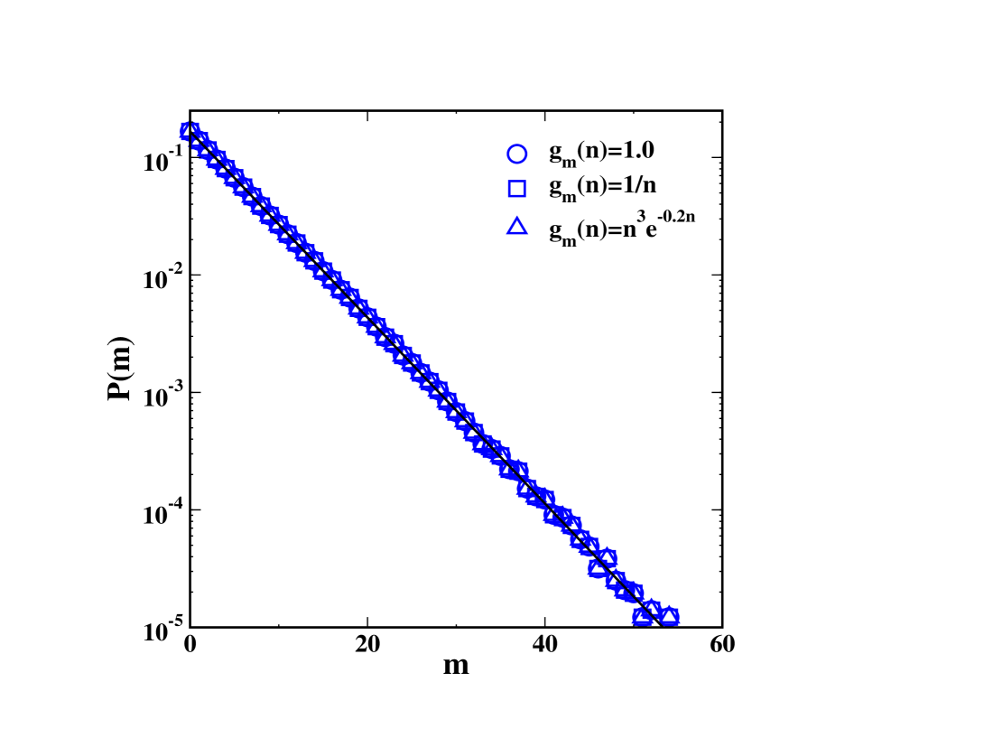
First, we present results for the kernel $g_{m}(n)=g(n)$, discussed in Sec. 2.1. In Fig. 1, we plot $P(m)$ vs. $m$ obtained from 1-$d$ MC simulations with $\rho=5$ and three different functional forms of $g_{m}(n)=1,1/n,n^{3}e^{-0.2n}$ and $\rho=5$. The MC data sets are numerically coincident with each other. They are also in excellent agreement with the 1-chip solution in Eq. (11) (denoted as a solid line), which was obtained from the corresponding MF equations. Our subsequent results also show that the MC data is described very well by the solutions of the corresponding MF equations, even for $d=1$. This demonstrates that the MF equations are exact in the present context emz06 .

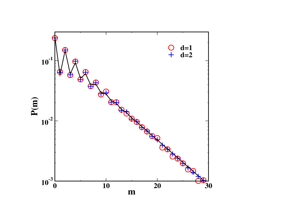
Second, we present results for the (1+2)-chip model discussed in Sec. 2.2. Fig. 2 shows the steady-state distributions obtained from 1-$d$ and 2-$d$ MC simulations with $\rho=5$, and $w_{1}=6,w_{2}=0.5$ and $w_{3}=7$. The solid line denotes the result in Eq. (27) - the corresponding roots and coefficients are specified in the caption. The oscillatory structure of $P(m)$ arises as one of the roots is negative. For the wide range of parameter values we considered, one of the roots is always found to be negative.

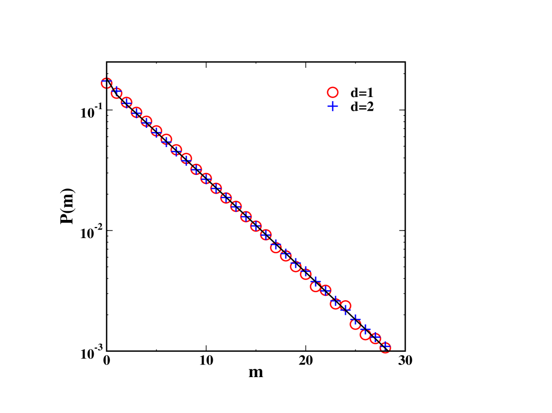
Next, let us consider the arbitrary kernel $g_{m}(n)=D(m)/n^{\alpha}$ with $D(m)$ determined from $\sum_{n=1}^{m}D(m)/n^{\alpha}=1$. Unlike our earlier models, this fragmentation kernel allows diffusion, which corresponds to the movement of the entire mass $m$ at a site to a randomly chosen neighbor. In Fig. 3, we show $P(m)$ vs. $m$ from MC simulations in $d=1,2$ with $\alpha=3$ and $\rho=5$. The solid line denotes the analytical result for the analogous ($1+2+3$)-chip model with $w_{i}$’s specified in the caption. Clearly, the ($1+2+3$)-chip approximation captures the original model rather well – this is true for $\alpha\gtrsim 2$.

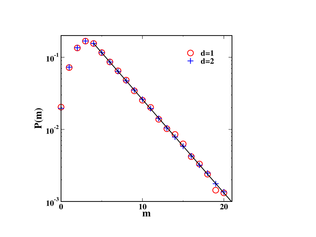
Finally, in Fig. 4, we show $P(m)$ vs. $m$ from MC simulations in $d=1,2$ for the $1$-chip model with different chip rates upto $m\geqslant 5$, i.e., $g_{m}(n)=\delta_{n,1}[w_{1}\delta_{m,1}+w_{2}\delta_{m,2}+w_{3}\delta_{m,3}+w_{4}\delta_{m,4}+w_{5}\theta(m-5)]$. We show results for $\rho=5$ and the $w_{i}$’s are specified in the caption. The solid line denotes the analytical solution obtained by generalizing the solution in Eqs. (50)-(51). This solution is exponential for $m\geqslant 4$.

IV Summary and Discussion

We conclude this paper with a summary and discussion of the results presented here. We have studied the steady-state distributions [$P(m)$ vs. $m$] for mass-transport models with multiple-chipping processes which depend upon the masses of the departure sites and the chips. These models are relevant for a variety of physical applications. In general, a site with mass $m$ could have 1, 2, 3,.., $m$ units of mass chip with different rates and aggregate with a neighbor. In this context, we study $k$-chip processes (where $k$ $=$ 1,2,3,…) and combinations thereof. We undertake Monte Carlo (MC) simulations of these models, and analytically study the steady-state solutions of the corresponding mean-field (MF) equations. Our MC results are in excellent agreement with the MF solutions, demonstrating that MF theory is exact in this context. This is true even when the kernels are not factorizable emz06 , and requires further investigation.

The steady-state distribution of the $k$-chip models has $k$ branches, each of which decays exponentially with the same slope. We find that a large class of chipping kernels, where $g_{m}(n)$ is independent of $m$, gives rise to an exponentially-decaying distribution: $P(m)=(1+\rho)^{-1}[\rho/(1+\rho)]^{m}$, where $\rho$ is the mass density. This is also the MF solution for the 1-chip model, where one unit of mass fragments from a site and aggregates with a randomly-chosen nearest-neighbor.

We have also studied models with a combination of 1-chip, 2-chip and 3-chip processes. The steady-state distributions of the $(1+2)$-chip model and $(1+2+3)$-chip model are sums of two exponential functions and three exponential functions, respectively. We expect the steady-state distribution of the $(1+2+\ldots+k)$-chip model to be a sum of $k$ exponentially-decaying functions. We have also examined several limiting cases of the above models. Our conclusion is that the steady-state distribution is sensitive to slight changes in the chipping kernel.

Finally, it is relevant to discuss physical processes which give rise to multi-exponential mass distributions vs. power-law distributions. Power laws have been observed in a class of mass-transport models where single-particle adsorption or chipping processes and (mass-independent) diffusion processes maintain a delicate balance between the lower and upper ends of the mass spectrum takayasu1 ; takayasu2 ; sk1 . On the other hand, mass-dependent fragmentation and aggregation precludes this balance. Consequently, all our models exhibit exponential distributions. These would be relevant in the context of ion-beam and sputter-deposited nanostructures, animal group distributions, polymerization, gelation and complex networks.

Acknowledgments

GPS and VB would like to acknowledge the support of CSIR Grant No. 03(1077)/06/EMR-II.

Figure 1: Steady-state probability distributions [$P(m)$ vs. $m$] from $d=1$ MC simulations with three different forms of $g_{m}(n)$. The data sets are plotted on a linear-logarithmic scale. The details of the MC simulations are provided in the text. The mass density is $\rho=5$. The solid line denotes the 1-chip solution in Eq. (11).

Figure 2: Plot of $P(m)$ vs. $m$ for the (1+2)-chip model, obtained from MC simulations in $d=1,2$ with $\rho=5$. We used $g_{m}(n)$ in Eq. (12) with $w_{1}=6,w_{2}=0.5$ and $w_{3}=7$. The solid line denotes the solution in Eq. (27) with $x_{1}=0.8427$, $x_{2}=-0.6498$, $A_{1}=0.1475$, $A_{2}=0.1021$.

Figure 3: Plot of $P(m)$ vs. $m$, obtained from MC simulations in $d=1,2$ with kernel $g_{m}(n)=D(m)/n^{\alpha}$ [where $D(m)^{-1}=\sum_{n=1}^{m}n^{-\alpha}$ ] for $\alpha=3$ and $\rho=5$. The solid line denotes the result for the analogous (1+2+3)-chip model with $w_{1}=1$, $w_{2}=8/9$, $w_{3}=1/9$, $w_{4}=216/251$, $w_{5}=27/251$ and $w_{6}=8/251$. The solution is a sum of three exponentials with $x_{1}=0.8372$, $x_{2}=-0.0594-0.1263i$, $x_{3}=-0.0594+0.1263i$, $A_{1}=0.1590$, $A_{2}=0.0118+0.0090i$, $A_{3}=0.0118-0.0090i$.

Figure 4: Plot of $P(m)$ vs. $m$ for the $1$-chip model with different chip rates upto $m\geqslant 5$. The symbols denote MC simulation results in $d=1,2$ with $\rho=5$ and $w_{1}=1$, $w_{2}=2$, $w_{3}=3$, $w_{4}=4$, $w_{5}=5$. The solid line denotes the generalization of Eqs. (50)-(51). The solution decays exponentially for $m\geqslant 4$, $P(m)=0.5133\times(0.7421)^{m}$.

References

- (1) Kinetics of Ordering and Growth at Surfaces, edited by M. Lagally, Vol. 239 of NATO Advanced Study Institute, Series B: Physics (Plenum, New York, 1990).
- (2) Morphological Organization of Epitaxial Growth and Removal, edited by Z. Zang and M.G. Lagally (World Scientific, Singapore, 1998).
- (3) J. A. Venables, Philos. Mag. 27, 697 (1973).
- (4) M. C. Bartelt and J. W. Evans, Phys. Rev. B 46, 12675 (1992).
- (5) G. S. Bales and D. C. Chrzan, Phys. Rev. B 50, 6057 (1994); Phys. Rev. Lett. 74, 4879 (1995).
- (6) L. Kuipers and R. E. Palmer, Phys. Rev. B 53, R7646 (1996).
- (7) H. Takayasu, I. Nishikawa, and H. Tasaki, Phys. Rev. A 37, 3110 (1988).
- (8) H. Takayasu, Phys. Rev. Lett. 63, 2563 (1989).
- (9) S. N. Majumdar, S. Krishnamurthy, and M. Barma, Phys. Rev. Lett. 81, 3691 (1998).
- (10) M. Rusanen, I. T. Koponen and J. Asikainen, Eur. Phys. J. B 36, 567 (2003).
- (11) P. Blandin, Phys. Rev. B 47, 13687 (1993).
- (12) P. Blandin, C. Massobrio and P. Ballone, Phys. Rev. Lett. 72, 3072 (1994).
- (13) H. Röder, H. Brune and K. Kern, Phys. Rev. Lett. 73, 2143 (1994).
- (14) A. Wucher, A. D. Bekkerman, N. K. Dzhemilev, S. V. Verkhoturov and I. V. Veryovkin, Nucl. Instr. Meth. B 140 311 (1998); A. Wucher, N. K. Dzhemilev, I. V. Veryovkin and S. V. Verkhoturov, Nucl. Instr. Meth. B 149 285 (1994).
- (15) We have checked this by fitting exponential distributions to the experimental data in blandin2 .
- (16) P.K. Kuiri, B. Joseph, H. P. Lenka, G. Sahu, J. Ghatak, D. Kanjilal and D. P. Mahapatra, Phys. Rev. Lett. 100, 245501 (2008).
- (17) E. Bonabeau, L. Dagorn, and P. Fre´on, Proc. Natl. Acad. Sci. U.S.A. 96, 4472 (1999).
- (18) E. Bonabeau and L. Dagorn, Phys. Rev. E 51, R5220 (1995).
- (19) R.M. Ziff, J. Stat Phys. 23, 241-263 (1980).
- (20) S. Kwon, S. Lee, and Y. Kim, Phys. Rev. E 73, 056102 (2006); ibid 78, 036113 (2008).
- (21) P. W. Davies, M. A. Quinlan and G. A. Samorjai, Surf. Sci. 121, 290 (1982).
- (22) G. P. Shrivastav, V. Banerjee and S. Puri, Phase Transitions 83, 140 (2010).
- (23) S.N. Majumdar, S. Krishnamurthy and M. Barma, J. Stat. Phys. 99, 1 (2000).
- (24) R. Rajesh, D. Das, B. Chakraborty and M. Barma, Phys. Rev. E 66, 056104 (2002).
- (25) M.R. Evans, S.N. Majumdar and R.K.P. Zia, J. Phys. A: Math. Gen. 39, 4859 (2006).
- (26) Handbook of Mathematical Functions, edited by M. Abramowitz and I. A. Stegun, (Dover, New York, 1972).