Nonparametric Dark Energy Reconstruction from Supernova Data
Abstract
Understanding the origin of the accelerated expansion of the Universe poses one of the greatest challenges in physics today. Lacking a compelling fundamental theory to test, observational efforts are targeted at a better characterization of the underlying cause. If a new form of mass-energy, dark energy, is driving the acceleration, the redshift evolution of the equation of state parameter will hold essential clues as to its origin. To best exploit data from observations it is necessary to develop a robust and accurate reconstruction approach, with controlled errors, for . We introduce a new, nonparametric method for solving the associated statistical inverse problem based on Gaussian Process modeling and Markov chain Monte Carlo sampling. Applying this method to recent supernova measurements, we reconstruct the continuous history of out to redshift .
pacs:
98.80.-k, 02.50.-rLittle more than a decade has passed after supernova observations first found evidence for the accelerated expansion of the Universe riessperl . Since confirmed by different probes, this remarkable discovery has been hailed as the harbinger of a revolution in fundamental physics and cosmology. Cosmic acceleration demands completely new physics – it challenges basic notions of quantum theory, general relativity, and assumptions regarding the fundamental make-up of matter. Currently, the two most popular explanations are a dark energy, usually modeled by a scalar field, or a modification of general relativity on cosmic length scales. In the absence of a compelling candidate theory to explain the observations, the target of current and future cosmological missions is to characterize the underlying cause for the accelerated expansion. In the case of dark energy, the aim is to constrain the equation of state parameter and its possible evolution. A deviation from would provide clues pointing to the origin of the accelerated expansion. (Currently, observations are consistent with a cosmological constant, , at the 10% level hicken09 .)
In order to extract useful information from cosmological data, a reliable and robust reconstruction method for is crucial. Here, we introduce a nonparametric technique based on Gaussian Process (GP) modeling and Markov chain Monte Carlo (MCMC) sampling, and apply it to supernova data. GPs extend the multivariate Gaussian distribution to function spaces, with inference taking place in the space of functions. The defining property of a GP is that the vector that corresponds to the process at any finite collection of points follows a multivariate Gaussian distribution. Gaussian processes are elements of an infinite dimensional space, and can be used as the basis for a nonparametric reconstruction method. GPs are characterized by mean and covariance functions, defined by a small number of hyperparameters gprefs . The covariance function controls aspects such as roughness of the candidate functions and the length scales on which they can change; aside from this, their shapes are arbitrary. Bayesian estimation simultaneously evaluates the GP hyperparameters (so-called to prevent confusion with the parameters that define a parametric method) together with quantities of physical interest.
For supernovae, the reconstruction task can be summarized as follows. The data is given in the form of the distance modulus defined as:
| (1) |
where and are the apparent and absolute magnitudes. The luminosity distance is connected to the Hubble expansion rate , and thus to , via:
where . Note that supernovae cannot be used to determine in the absence of an independent distance measurement. Thus it remains an unknown and can be absorbed in a redefinition of the absolute magnitude: . The used to obtain is not the physical value, but a certain fixed constant assumed in the observational analysis. For the dataset analyzed below hicken09 , km/s/Mpc. Since we will work with and not with directly, the numerical value for does not enter in our analysis. We allow for a free constant, in Eqn. (1), accounting for the uncertainty in the absolute calibration of the data, and for which we choose a uniform prior between . We assume spatial flatness as an “inflation prior”; strong constraints on spatial flatness exist from combining cosmic microwave background (CMB) and baryon acoustic oscillation (BAO) measurements komatsu . The prior on is also informed by the 7-year WMAP analysis komatsu for a CDM model combining CMB, BAO, and measurements. Since our assumptions on are less strict than we broaden the nominal range by a factor of two, leading to a Gaussian prior with mean 0.27 and standard deviation of 0.04.
Reconstruction is a classic statistical inverse problem for the nonlinear (smoothing) operator of Eqn. (Nonparametric Dark Energy Reconstruction from Supernova Data), where one solves for the function and for the parameter , given a finite set of noisy data for . Different strategies may be followed to arrive at a tractable formulation. (i) Assume a parameterized form for and estimate the associated parameters. This approach is the most commonly used currently; the parametric forms either assume or allow for a fixed redshift variation such as , where and are constants linder03 . (ii) Pick a simple local basis representation for (bins, wavelets), and estimate the associated coefficients (effectively a piecewise constant description), using Principal Component Analysis (PCA) if needed, to work with eigenmodes defined as linear combinations of bins huterer04 ; hojjati09 . (iii) Follow a procedure similar to (ii) – without PCA – but actually use (filtered) numerical derivatives to estimate daly03 . (iv) Use a distribution over (random) functions that can represent and estimate the statistical properties thereof, given observed data. Methods (i), (ii), and (iv) can all be carried out using a Bayesian viewpoint and exploring posteriors by MCMC methods, whereas (iii) – as presented in the literature – represents a different class of approach to the inverse problem. Taking numerical derivatives is generally a difficult task and a corresponding error theory seems hard to develop. Approach (i) can encounter difficulties if has a nontrivial evolution. The finite parameterization and the specific functional form assumed can bias results for the temporal behavior of simpson06 . Methods (ii) and (iv) apply different philosophies – (ii) applies a local view of the reconstruction ( bins), whereas (iv) attempts to sample the posterior continuously in . In a mild sense, the choice of a piecewise continuous representation in (ii) – of which, is just the one-bin limit – can force an unphysical view of , since the actual is not piecewise constant. In contrast, method (iv) while fully nonparametric, is potentially more general and flexible compared to the other methods.
Our new GP modeling-based approach is a realization of method (iv). It enables the identification of nontrivial redshift dependences in reliably, if they exist (Ref. holsclaw09 shows examples based on simulated data). The central idea is to assign prior probabilities to classes of functions via GPs and to take advantage of the particular integral structure of Eqn. (Nonparametric Dark Energy Reconstruction from Supernova Data), again using GPs. Employing a Bayesian approach to explore posterior distributions over the functions via MCMC we not only obtain a family of continuous realizations for but at the same time optimize the GP model hyperparameters, informed by the actual data, comprehensively propagating all estimation uncertainties.
One may wonder whether a general nonparametric reconstruction must involve taking a second derivative of the data in some way. This is true only in a formal sense – the approach described here does not involve any derivatives. Instead, we invert an integral equation, ill-posed because the operator to be treated is a complicated smoothing operator involving two integrals. To make the problem well-behaved we make mild continuity assumptions about which are justified if the origin of dark energy is to be described by a reasonable physical model.


As previously noted, a GP model assumes that , for any set of redshifts , follow a multivariate Gaussian distribution specified by mean and covariance functions gprefs . Here we use a mean of negative one as the prior and exponential family covariance functions written as ( being a numerical constant):
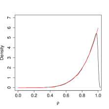
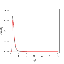
The hyperparameters and , and the parameters defining the likelihood, are determined by the data. The value of influences the smoothness of the GP realizations: for , the realizations are smooth with infinitely many derivatives (this covariance function corresponds to using an infinite number of Gaussian basis functions), while leads to rougher realizations suited to modeling continuous non-(mean-squared)-differentiable functions. We use both values in our analysis, the results being very similar. The form of the covariance function is unrelated to the shape of the GP sampling functions, as determined by the data, so no particular behavior is assumed for . There is no loss of generality in fixing the (statistical ensemble) GP mean, as any variation imposed by the data appears in the covariance function. Fixing the mean has the advantage of improving the stability of the MCMC (we explored other means and found very similar results). We stress that even though the mean is fixed, each GP realization will actually have a different mean with a spread controlled by as shown in Figure 1. The constant has a prior of and has a vague Inverse Gamma prior . The probability distribution of the prior is given by and for the prior by , with . We show the priors for and and their posterior distribution in Figure 1.
Following the notation of Eqn. (Nonparametric Dark Energy Reconstruction from Supernova Data) we set up the following GP for :
Recall that we have to integrate over (Eqn. Nonparametric Dark Energy Reconstruction from Supernova Data):
| (3) |
We use the fact that the integral of a GP is also a GP with mean and covariance dependent on the original GP gprefs . Using that result, we set up a second GP for :
The mean value for this GP is simply obtained by solving the integral in Eqn. (3) for the mean value of the GP for , here taken to be negative one. As mentioned earlier, even though the ensemble mean is fixed to a constant value at any , each GP realization is not mean-zero (over ). We show the distribution of the mean for the different realizations in Figure 1 demonstrating a wide spread between -2 and -0.6. In addition, we used simulated data with a time-varying equation of state to check that the choice of the mean does not bias the results.


We can now construct a joint GP for and :
a multi-variate normal (MVN) distribution with
| (4) | |||||
| (5) | |||||
| (6) |
The mean for given can be found through the following relation:
Now only the outer integral is left to be solved for in Eqn. (Nonparametric Dark Energy Reconstruction from Supernova Data), and this can be computed by standard numerical methods. (Note that the computationally expensive double integral for as defined in Eqn. (4) does not need to be performed.) The GP prior can now be combined with a likelihood function to obtain a posterior that can be sampled by MCMC methods. Details of our GP-based MCMC implementation are provided in the supplementary material supp .
For our specific analysis we focus on a recent composite supernova dataset, provided by Hicken et al. hicken09 . This dataset combines the so-called Union dataset union with new measurements of low redshift supernovae to form the Constitution set. The dataset has been analyzed in Ref. hicken09 using different light curve fitters for the supernova light curves; our analysis uses results from the SALT fitter (Table 1 in Ref. hicken09 , which includes estimates for the error for the distance modulus – the tables contain what is referred to in Ref. hicken09 as the “minimal cut”).
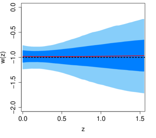
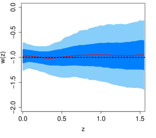
Our final results for are shown in Figure 2. The upper panel shows the results from a GP model with a Gaussian covariance function () while the results in the lower panel are based on an exponential covariance function (). The results are very similar, the Gaussian covariance function leading to a slightly smoother prediction. The mean value of is very close to -1 at redshifts close to zero and rises slightly at redshift . Within our estimated errors, the results are consistent with a cosmological constant . Note, however, that realizations of with nontrivial -dependence are not excluded; as observations improve the allowed range of variability will be further constrained. In Ref. hicken09 a combined analysis of supernova data and baryon acoustic oscillation measurements is carried out. Assuming , the SALT-based dataset yields consistent with our findings.
To summarize, we have presented a new, nonparametric reconstruction technique for the dark energy equation of state and applied it to current supernova observations. The GP-based method can be used to determine the most probable behavior of and to infer how likely a target trajectory is given the current data. Thus it can be used to accept or reject classes of models. The method allows adjusting of smoothness assumptions regarding ; priors on the GP hyperparameters control the allowed arbitrariness (e.g., degree of differentiability). Robustness of the results obtained can be checked by varying these priors. Our results for are consistent with a cosmological constant, with no evidence for a systematic mean evolution in with redshift, although variations within our error limits cannot be ruled out. We have carried out careful tests to ensure that our choices of priors and hyperparameters do not alter the results. Our method possesses several advantages: it avoids artificial biases due to restricted parametric assumptions for , it does not lose information about the data by smoothing it, and it does not introduce arbitrariness (and lack of error control) in reconstruction by representing the data using a certain number of bins, or cutting off information by using a restricted set of basis functions to represent the data. The technique can be easily extended to fold in data from CMB and BAO observations; work in this direction is currently in progress. The GP-based MCMC procedure can be integrated within supernova analysis frameworks, e.g., SNANA snana as a cosmology fitter, following the general methodology presented in Ref. habib07 .
We thank the LANL/UCSC Institute for Scalable Scientific Data Management for supporting this work. Partial support by the DOE under contract W-7405-ENG-36 is also acknowledged. UA, SH, KH, and DH acknowledge support from the LDRD program at LANL; KH acknowledges support from the NASA Theory program. SH and KH thank the Aspen Center for Physics, where part of this work was carried out. We are indebted to Andy Albrecht, Josh Frieman, Adrian Pope, Martin White, and Michael Wood-Vasey for insightful discussions.
References
- (1) A.G. Riess et al., Astron. J. 116, 1009 (1998); S. Perlmutter et al., Astrophys. J. 517, 565 (1999).
- (2) M. Hicken et al., Astrophys J. 700, 1097 (2009).
- (3) S. Banerjee, B.P. Carlin, and A.E. Gelfand, Hierarchical Modeling and Analysis for Spatial Data, New York: Chapman and Hall (2004); C.E. Rasmussen and K.I. Williams, Gaussian Processes for Machine Learning, Boston: MIT Press (2006).
- (4) E. Komatsu et al., arXiv:1001.4538 [astro-ph.CO].
- (5) M. Chevallier and D. Polarski, Int. J. Mod. Phys. D 10, 213 (2001); E.V. Linder, Phys. Rev. Lett. 90, 091301 (2003).
- (6) D. Huterer and A. Cooray, Phys. Rev. D 71, 023506 (2005).
- (7) A. Hojjati, L. Pogosian, and G.-B. Zhao, JCAP 1004, 007 (2010).
- (8) R.A. Daly and S.G. Djorgovski, Astrophys. J. 597, 9 (2003); A. Shafieloo, U. Alam, V. Sahni, and A.A. Starobinsky, Mon. Not. Roy. Astron. Soc. 366, 1081 (2006).
- (9) F. Simpson and S.L. Bridle, Phys. Rev. D 73, 083001 (2006).
- (10) T. Holsclaw, U. Alam, B. Sansó, H. Lee, K. Heitmann, S. Habib, and D. Higdon, Phys. Rev. D 82, 103502 (2010).
- (11) Implementation details of the GP-based MCMC procedure are provided in the supplementary material at http://link.aps.org/supplemental/XXX.
- (12) M. Kowalski et al., Astrophys. J. 686, 749 (2008).
- (13) R. Kessler et al. Publ. Astron. Soc. Pac. 121, 1028 (2009).
- (14) S. Habib, K. Heitmann, D. Higdon, C. Nakhleh, and B. Williams, Phys. Rev. D 76, 083503 (2007).