Study of the scaling properties in SU(2) gauge theory with eight flavors

Abstract:

We present our preliminary study of the SU(2) gauge theory with 8 flavors of fermions in fundamental representation. This theory could be a candidate of the gauge theory with conformal fixed point. By using Wilson/Polyakov loop in a finite volume with twisted boundary conditions, we study the renormalization group flow of the gauge coupling constant. Our calculation gives consistent result with the perturbative prediction of the running coupling in the weak coupling region. We investigate a possible signal for conformal behavior in the strong coupling region.

1 Introduction

There has been a lot of interest in the non-supersymmetric gauge theories with non-trivial infrared fixed point (IRFP) [1, 2]. Such a theory could play an important role in the phenomenology of the physics beyond the standard model. Since the existence of the IRFP gives slow running of the gauge coupling, it may be a possible candidate of walking technicolor model [3, 4, 5, 6, 7]. Within the framework of the walking technicolor scenario, the large anomalous dimensions for the bilinear operators could give a possible way to resolve the tension between the realistic quark masses and the suppressed flavor changing neutral current.

SU(N) gauge theories with many flavors have been considered as traditional candidates for the walking technicolor scenario. In fact, the two-loop perturbative $\beta$ function predicts the existence of the IRFP within a certain region of the number of fermions which is so called conformal window. Near the conformal window, the anomalous dimension is expected to be enhanced from the Schwinger-Dyson analysis. In addition, in such a theory the contribution to the electroweak S parameter might be suppressed in contrast to QCD like theories. These features are favorable from the view point of model construction of the realistic dynamical electroweak breaking. Furthermore, once a theory has an IRFP, it does not break the chiral symmetry and should be inside the conformal window. It is helpful to understand the phase structure of the gauge theory, i.e. whether a model is in the chiral symmetry broken phase or not. The identification of the conformal gauge theory itself is interesting beyond phenomenological issues.

In the lattice calculation, whether a certain model has an IRFP or not can be answered from first principle. A simple way to identify the conformality is an analysis of the renormalization group flow of the gauge coupling constant. Recently non-perturbative lattice calculations of the running coupling constant are widely investigated. There are several methods in analysis, e.g. the Schroedinger functional (SF) running coupling scheme [8, 9] and twisted Polyakov loop method. There has been lots of studies of the running coupling constant e.g. $n_{f}=8,12$ and $16$ flavor models in SU(3) [10, 11], two flavors of adjoint fermions in SU(2) gauge group [12], and for a recent study of the SU(2) with fundamental six-flavor model, see Ref. [13].

In this report, we study the infrared behavior in $n_{f}=8$ flavor SU(2) model. We employ twisted boundary conditions in which the methods for calculation of the renormalized coupling can be defined. This twisted boundary condition does not need the additional boundary terms in contrast to SF boundary so the measured values have no ${O}(a)$ contribution. Therefore we could obtain systematically reliable results. Using the finite volume scaling method, we obtain the renormalization group flow of the gauge coupling constant and study its low-energy behavior. In order to see the non-perturbative features of the theory, we investigate the possible signals for the IRFP by using the growth rate of the running coupling constant. This quantity is easy to compare with the one obtained from the perturbative calculations.

This report is organized as follows. In section 2, we introduce two methods for calculation of the running coupling constant in twisted boundary conditions; one is obtained from the Polyakov loop correlation functions (TPL scheme) and another is from the Wilson loop. In section 3, we show some numerical results on the running coupling constant in 8-flavor SU(2) gauge model. In section 4, we show our preliminary study of the growth rate of the running coupling constant for each of the renormalized coupling. Finally in section 5, we summarize our results.

2 The running coupling in twisted boundary condition

In this section, we present the definition of the twisted boundary conditions for both of link and fermion variables in SU(2) gauge theory. Here we consider twisted boundary conditions [14] for the link variables in $x$ and $y$ directions on the lattice;

$$U_{\mu}(x+\hat{\nu}L/a)=\Omega_{\nu}U_{\mu}\Omega_{\nu}^{\dagger},\ (\nu=x,y)$$ (1)

where the twist matrices $\Omega_{\mu}$ are introduced as follows,

$$\Omega_{x}\Omega_{y}=-\Omega_{y}\Omega_{x},\ \ \Omega_{\mu}\Omega_{\mu}^{\dagger}=1,\ \ \left(\Omega_{\mu}\right)^{2}=-1,\ \ \rm{Tr}\Omega_{\mu}=0.$$ (2)

The consistency of the twisted boundary condition for fermions should accompany with the additional ’smell’ flavor degrees of freedom. We take the following boundary conditions

$$\psi_{\alpha}^{a}(x+\hat{\nu}L/a)=e^{i\pi/2}\Omega_{\nu}^{ab}\psi_{\beta}^{b}\left(\Omega_{\nu}^{\dagger}\right)_{\beta\alpha},$$ (3)

for $\nu=x,y$ directions. Here the indices of $\alpha,\beta$ and $a,b$ represent the smell degree $N_{s}$ and color $N_{c}$. The number of smell should be multiples of the number of color. We take $N_{s}=N_{c}=2$.

Then the TPL scheme coupling [15] is defined as

$$g^{2}_{TPL}=\frac{1}{k}\frac{\langle\sum_{y,z}P_{x}(y,z,L/2a)P_{x}(0,0,0)^{\dagger}\rangle}{\langle\sum_{x,y}P_{z}(x,y,L/2a)P_{z}(0,0,0)^{\dagger}\rangle},$$ (4)

where $P_{x,z}$ are the Polyakov loop in the twisted and untwisted directions defined in a gauge invariant way. For instance $P_{x}$ is given by

$$P_{x}(y,z,t)=\rm{Tr}\left(\prod_{j}U_{x}(x=j,y,z,t)\Omega_{x}e^{i\pi y/L}\right).$$ (5)

The coefficient $k$ is obtained by analytic calculation which gives $k=0.0172\cdots$ .

2.1 Method using Wilson loop

We also introduce the method for the coupling constant by using Wilson loop [16]. We first use the Creutz ratio in a finite volume $(L/a)^{4}$ as

$$\chi(R/a+1/2,L/a)\equiv\ln{\left(\frac{W(R/a+1,R/a+1)W(R,R)}{W(R/a+1,R)W(R/a,R/a+1)}\right)},$$ (6)

where $W(R/a,T/a)$ means the rectangle Wilson loop. Each of $R/a$ and $T/a$ means the length of the Wilson loop for each different direction. To fix the scheme we consider a measurement of the Wilson loop for untwisted-untwisted directions. Taking different directions such as twisted-twisted direction corresponds to the different scheme of defining of the renormalized couplings. Then this quantity is proportional to the gauge coupling $g^{2}$ at leading order. By multiplying the tree level matching factor $1/k$, renormalized gauge coupling constant can be defined by

$$g^{2}_{W}(L/a,R/L+1/2)=\chi(R/a+1/2,L/a)/k.$$ (7)

Here $g^{2}_{W}$ is a function of the ratio $(R/L+1/2)\equiv r$, $L/a$ and physical volume $L(=1/\mu)$ where $\mu$ is the energy scale. In order to obtain the renormalized coupling $g^{2}_{W}$ in a finite volume, we fix the value of r to an appropriate value. In our case, we take $r=0.25$.

Since $\chi(r,L/a)$ itself has a systematic artifact from discretization [16, 11], it is better to improve $g^{2}_{W}(r)$ by using discretized value of the leading factor $k(r)$ instead of its continuum value which is calculated in a lattice perturbation [11]. While both the $k(r)$ and $\chi(r)$ contain large lattice artifacts, some of them may be canceled each other and the ratio $\chi(r)/k(r)$ could behave as a smooth continuous function of $r$.

3 Simulation detail

We carry out the measurements of the coupling from TPL and Wilson loop methods. Our simulations are performed on $L=6,8,10,12,14,16,18$ lattices with plaquette gauge action with one massless staggered fermion with twisted boundary condition which corresponds 8-flavor fermions. The gauge configurations are generated by the Hybrid Monte Carlo algorithm. We take several values of $\beta=1.3\sim 15$ for each of lattices. We accumulate about $2\sim 5\times 10^{4}$ trajectories for $L=6\sim 14$ and about $5,000\sim 20,000$ trajectories for $L=16\sim 18$. Then we take every trajectory for the measurement of the Wilson loop and Polyakov loop. The error estimation is made by a standard Jackknife analysis with $O(10^{3})$ bin size.

As defined in the previous section, the TPL gauge coupling is obtained directly from the configurations as long as $L/a$ is even. While in the case of $L=6,10,14,18$, we can obtain $g_{W}^{2}$ directly, in the case of $L=8,12,16$, we need to interpolate the Creutz ratio as a function of $r$. Since $k(r)$ becomes zero at $r=1/2$, $g^{2}_{W}(r)$ blow up at $r=1/2$ and we find that the function $g^{2}_{W}(r)$ is reasonably fitted by using the pole type functions as $g^{2}_{W}(r)\sim\frac{f(r)}{r-1/2}$ where $f(r)$ is a polynomial function with $f(r=1/2)\neq 0$. Hence we obtain the renormalized gauge couplings from Wilson loop method even in small volumes .

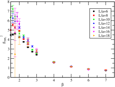
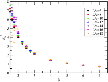
Thus we obtain both the results of the renormalized couplings defined by two methods. The results are shown in Fig.1. As shown here, both show similar $\beta$ dependence and they are close to each other in the weak coupling region. We find the relative error of the Wilson loop coupling is about $1/5\sim 1/10$ of that of TPL coupling even in small $\beta$ and large $L/a$ regions. As it is important to know the infrared region of this model, now we concentrate on the analysis of the coupling from Wilson loop.

Figure 1: The renormalized gauge couplings for each $\beta$ and $L$. In the left panel, the data show the TPL gauge couplings, in the right panel, the data show the Wilson loop couplings.

4 Result

In order to study the renormalization flow of the running couplings, we use the finite scaling method. First we define the step scaling function for the gauge coupling as

$$\Sigma(u,s,a/L)=\left.g^{2}(\beta,sL/a)\right|_{g^{2}(\beta,L/a)=u},$$ (8)

where parameter $s$ is the scaling parameter. In our analysis, we set $s=3/2$. We obtain four data of $g^{2}(\beta,L/a)$ at a fixed $u$ for coarse lattices such that $L/a=6,8,10,12$ by tuning $\beta$. In the case of Wilson loop, it is easy to interpolate to the arbitrary value of $\beta$ by using the following fit function as

$$g^{2}_{W}(\beta)=\sum_{i=1}^{n}\frac{c_{i}}{(\beta-\beta_{0})^{i}}.$$ (9)

Our fitting procedure is as follows. First we carry out the fit of $\beta$ dependence of gauge couplings at each of fixed lattices with the free parameters $\beta_{0}$ and $c_{i}$. We use typically $6\sim 8$ free parameters to fit the results. Fit range of $\beta$ is taken as $\beta=1.5\sim 15$. Thus we interpolate $g^{2}(\beta,L/a)$ at arbitrary value of $\beta$ for each of lattices. In order to obtain the $g^{2}(\beta,L/a)$ for unmeasured lattices of $L/a=9$ and $15$, we also fit the volume dependence of $g^{2}(\beta,a/L)$ at fixed $\beta$ by the following polynomial functions

$$g^{2}_{W}(\beta,L/a)=d_{0}+d_{1}L/a+d_{2}(L/a)^{2},$$ (10)

where the coefficients $d_{i}$ are free parameters. In these fits we use four data points of $L/a=6,8,10,12$ for obtaining the value at $L/a=9$ and $L/a=12,14,16,18$ for $L/a=15$, respectively. Finally using four data points of $\Sigma(u,3/2,a/L)$ we take continuum extrapolation and obtain continuum step scaling function $\sigma(u)$ defined by $\sigma(u)=\lim_{a/L\to 0}\Sigma(u,s,a/L)$. We try to carry out the continuum extrapolations by two ways; one is a linear extrapolation in terms of $(a/L)^{2}$ by using three data points of $a/L$ closing to the continuum limit, i.e. $a/L=1/12,1/15$ and $1/18$ and another is a quadratic extrapolation in terms of $(a/L)^{2}$ by using four data points.

Figure 2: The data shows the results of $\sigma(u)$ for each of lattices $L/a=9,12,15$ and $18$. The continuum extrapolation results for linear and quadratic fits are shown by blue and red curves, respectively. The solid line represent the initial values of $u$ ($u=0.8$ in left panel, $u=4.5$ in right panel). The dotted line represent the two-loop results of the $\sigma(u)$.

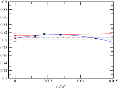
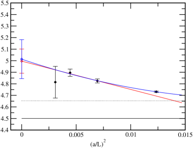
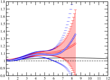
Here we show some results of the continuum extrapolation of $\Sigma(u)$. Figure 2 shows the continuum extrapolations of the $\Sigma(u,s,a/L)$ with $u=0.8$ (left panel) and $u=4.5$ (right panel). Figure 3 shows the result of the $\sigma(u)/u$. In the perturbative region the results at the continuum limit of linear and quadratic extrapolations $\sigma(u=0.8)$ gives consistent result with perturbative 2-loop continuum prediction. On the other hand, in the strong coupling region, We find the result of $\sigma(u)/u$ are larger than that of two-loop continuum perturbation. Although the two results are consistent with each other within $1\sigma$ level and also consistent with the IRFP above $g^{2}_{W}\sim 6$, because the growth rate is consistent with dashed line in Fig. 3, we can not yet conclude clearly that there is an IRFP due to its large statistical uncertainty. In order to determine the renormalization flow of $\sigma(u)$, the more statistics are needed especially in large lattices such as $a/L=1/16$ and $1/18$.

Figure 3: $\sigma(u)/u$ obtained by linear (blue) and quadratic (red) continuum extrapolation. The horizontal axis shows the initial value of $u=g^{2}_{W}$. The vertical axis show the result of $\sigma(u)/u$. For the reference we also show the two-loop perturbative results of the $\sigma(u)/u$ by solid curve. Dashed line represents $\sigma(u)=u$.

5 Summary

In this proceedings we reported on the infrared behavior of the SU(2) gauge theory with fermions of 8-flavor in the fundamental representation. We measured the renormalized gauge couplings defined in twisted boundary conditions. This twisted boundary condition does not need the additional boundary terms so the measured values have no $O(a)$ contribution. Using the finite volume scaling method, we obtained the renormalization group flow of the gauge coupling constant. We found that in the weak coupling region the running of gauge couplings gives consistent result with perturbative two-loop prediction. However, in the strong coupling we can not have conclusive results of the existence of the IRFP due to the large uncertainty.

The accuracy of our results could be improved by accumulation of more statistics. This may help to stabilize the continuum extrapolations of the running coupling and enable us to study the consistency of the two results obtained by two different methods which gives non-trivial check of the existence of the IRFP. We are also studying other physical quantities such as Wilson loop itself and fermion bilinear operators. They could also reveal some properties of the strong coupling gauge theories. These works are still ongoing [17].

Acknowledgements

Main numerical simulations are performed on Hitachi SR11000 and IBM System Blue Gene Solution at High Energy Accelerator Research Organization (KEK) under a support of its Large Scale Simulation Program (No. 09/10-22). This work is also performed by using NEC SX-8 at Yukawa Institute for Theoretical Physics (YITP), Kyoto University and at Research Center for Nuclear Physics (RCNP), Osaka University.

This work is supported in part by the Grants-in-Aid of the Japanese Ministry of Education, Culture, Sports, Science and Technology (No. 22740173, 21$\cdot$897), and the Grant-in-Aid of the Japanese Ministry for Scientific Research on Innovative Areas (No. 20105002, 20105005, 21105501, 21105508). C.-J.D. L. is supported by the National Science Council of Taiwan via grant 96-2122-M-009-020-MY3.

References

- [1] W. E. Caswell, Phys. Rev. Lett. 33, 244 (1974).
- [2] T. Banks and A. Zaks, Nucl. Phys. B 196, 189 (1982).
- [3] S. Weinberg, Phys. Rev. D 13, 974 (1976).
- [4] L. Susskind, Phys. Rev. D 20, 2619 (1979).
- [5] B. Holdom, Phys. Lett. B 150, 301 (1985).
- [6] K. Yamawaki, M. Bando and K. i. Matumoto, Phys. Rev. Lett. 56, 1335 (1986).
- [7] T. W. Appelquist, D. Karabali and L. C. R. Wijewardhana, Phys. Rev. Lett. 57, 957 (1986).
- [8] M. Luscher, P. Weisz and U. Wolff, Nucl. Phys. B 359, 221 (1991).
- [9] M. Luscher, R. Narayanan, P. Weisz and U. Wolff, Nucl. Phys. B 384, 168 (1992) [arXiv:hep-lat/9207009].
- [10] T. Appelquist, G. T. Fleming and E. T. Neil, Phys. Rev. Lett. 100, 171607 (2008) [Erratum-ibid. 102, 149902 (2009)] [arXiv:0712.0609 [hep-ph]]. T. Appelquist, G. T. Fleming and E. T. Neil, Phys. Rev. D 79, 076010 (2009) [arXiv:0901.3766 [hep-ph]].
- [11] Z. Fodor, K. Holland, J. Kuti, D. Nogradi and C. Schroeder, PoS LATTICE2008, 066 (2008) [arXiv:0809.4890 [hep-lat]].
- [12] A. J. Hietanen, K. Rummukainen and K. Tuominen, with two Phys. Rev. D 80, 094504 (2009) [arXiv:0904.0864 [hep-lat]].
- [13] F. Bursa, L. Del Debbio, L. Keegan, C. Pica and T. Pickup, arXiv:1007.3067 [hep-ph].
- [14] G. ’t Hooft, Nucl. Phys. B 153, 141 (1979).
- [15] G. M. de Divitiis, R. Frezzotti, M. Guagnelli and R. Petronzio, Nucl. Phys. B 422, 382 (1994) [arXiv:hep-lat/9312085]. G. M. de Divitiis, R. Frezzotti, M. Guagnelli and R. Petronzio, Nucl. Phys. B 433, 390 (1995) [arXiv:hep-lat/9407028].
- [16] E. Bilgici et al., Phys. Rev. D 80, 034507 (2009) [arXiv:0902.3768 [hep-lat]].
- [17] H. Ohki et al. in preparation.