Studying Frequency Relations of kHz QPOs for 4U 1636-53 and Sco X-1: Observations Confront Theories

Abstract

By fitting the frequencies of simultaneous lower and upper kilohertz Quasi-Periodic Oscillations (kHz QPOs) in two prototype neutron star QPO sources (4U 1636-536 and Sco X-1), we test the predictive power of all currently proposed QPO models. Models predict either a linear, power-law or any other relationship between the two frequencies. We found that for plausible neutron star parameters (mass and angular momentum), no model can satisfactorily reproduce the data, leading to very large chi-squared values in our fittings. Both for 4U 1636-53 and Sco X-1, this is largely due to the fact that the data significantly differ from a linear relationship. Some models perform relatively better but still have their own problems. Such a detailed comparison of data with models shall enable to identify routes for improving those models further.

1. Introduction

The launch of the X-ray timing satellite, Rossi X-ray Timing Explorer (RXTE), led to the discovery of kilohertz Quasi Periodic Oscillations (kHz QPOs) of low mass X-ray binaries (LMXBs) in their X-ray lightcurves. The frequencies of kHz QPOs range from a few hundreds to about one thousand Hz; its time-scale corresponds to the dynamical time of the innermost regions of the accretion flow. Thus such signals may carry crucial information about the central neutron star (NS), such as the mass, spin frequency, angular momentum, radius, magnetic fields and so on. Usually the twin kHz QPOs appear simultaneously and the lower and upper QPOs are almost directly proportional with each other (see e.g. van der Klis, 2006).

Various theoretical models have been proposed to account for the kHz QPO signals. Table 1 shows all the present models we collect. Although each model achieves its success to a certain extent, the origin of kHz QPOs is still highly debated. Furthermore many new models emerge in recent years, and systematic comparisons among them have not been well studied.

Table 1Present models.

Models	Reference
Sonic-point and spin-resonance	[1, 2, 3]
Orbital resonance (3 models)	[4, 5]
Precession (3 models)	[6, 7, 8]
Deformed-disk oscillation	[9]
‘-1r, -2v’ resonance	[10, 11]
Higher-order nonlinearity	[12]
Tidal disruption	[13]
Rayleigh-Taylor gravity wave	[14, 15]
MHD Alfvén wave oscillation	[16]
MHD	[17]
Moving hot spots	[18]

[1] Miller et al (1998); [2] Lamb and Miller (2001); [3] Lamb and Miller (2003); [4] Kluźniak and Abramowicz (2001); [5] Abramowicz et al (2003); [6] Stella and Vietri (1999); [7] Bursa (2005); [8] Stuchlík et al (2007); [9] Kato (2001); [10] Török et al (2007); [11] Bakala et al (2008); [12] Mukhopadhyay (2009); [13] Germanà et al (2009); [14] Osherovich and Titarchuk (1999); [15] Titarchuk (2003); [16] Zhang (2004); [17] Shi and Li (2009); [18] Bachetti et al (2010).

In view of this, we investigate systematically the predictive ability of the present kHz QPO models. We focus on those that predict the frequency relation of twin kHz QPOs. The moving hot spots model is not included. This model performs a 3D MHD simulations of the accretion around a NS. The simulations show that the moving hot spots on the surface of a NS can develop oscillations in the lightcurves. However, this model does not provide any analytic relation between the twin QPOs (Bachetti et al, 2010).

In this work, we measure the frequency relations of the twin kHz QPOs for 4U 1636-53 and Sco X-1, then fit the models with the measured results. We choose these two NS systems for several reasons. Firstly, both of them have strong kHz QPOs over a wide frequency range; both of them have been observed more than 10 years with RXTE. Thus the bias from the sample selection is minimized. Moreover, the different properties of these two sources allow us to discuss the predictive ability of the models. They are typical Atoll and Z source, respectively. The putative spin frequency for 4U 1636-53 is $581$ Hz (Strohmayer, 2001; Strohmayer and Markwardt, 2002), whereas the spin frequency of Sco X-1 remains unknown.

In the following, we firstly describe the data reduction procedure. Then we fit the frequency relations with all the available models. The predictions of NS properties in each model will be presented. Finally we discuss and conclude our investigation results.

2. Data Analysis

We have retrieved all the public archival data of the two sources with the Proportional Counter Array (PCA) on board RXTE. The observation time is from Feb. 28th, 1996 to Sep. 25th, 2007 for 4U 1636-53, and from May 5th, 1996 to Feb. 4th, 2006 for Sco X-1.

For 4U 1636-53, we use the event mode data for 1156 ObsIDs, with time resolution better than 256 $\mu$s and an energy band of 2-40 keV. With the similar analysis procedure in Barret et al (2006) and Boutelier et al (2009a), the PDS as well as the QPO parameters (peak frequency, width and amplitude) in each ObsID are obtained. For the ObsIDs with PDS containing the lower QPO, we track its time evolution in every 128 s. Following that in Barret et al (2005), all the 128 s PDS are aligned in every 30 Hz interval of the lower QPO with the shift-and-add technique (Méndez et al, 1998). Then we search for twin QPOs in each interval. For the ObsID with PDS containing only the upper QPOs, we directly align the PDS of each ObsID in every 30 Hz interval of upper QPO. Again the twin QPOs in each interval are searched. Finally, the two parts of results are combined and we obtain the frequency relation.

For Sco X-1, we analyze the Generic Binned mode data in 187 ObsIDs with time resolution better than 256 $\mu$s and an energy band of 2-40 keV. Considering the effects of the deadtime, we use a model of two Lorentzians plus a powerlaw to fit each PDS. The powerlaw component denotes the deadtime-modified Poisson noise; the Lorentzians account for the contribution of the twin kHz QPOs. We then apply the shift-and-add technique to the ObsID averaged PDS as described above on the upper QPOs’ frequency, because the span and significance of the upper QPOs are larger than that of the lower QPOs. The interval of shift-and-add is 50 Hz. Similar to the result in Méndez and van der Klis (2000), our frequency relation shows some subtle structure when the lower QPO is around 800 Hz.

3. Comparisons between Models and Data

In the following, we restrict the NS parameters $M\in[1.4,2.4]$ $M_{\odot}$ and $j\in[0,0.3]$ ($j\equiv{Jc/GM^{2}}$) in our fittings, corresponding to reasonable equations of state (EOS) of NSs (Lattimer & Prakash 2007), where $M$ and $j$ are the mass and dimensionless angular momentum parameter of a NS, respectively. The fitting results are summarized in Table 2. For some models, the best fitting values of $M$ and $j$ approach the upper or lower limits. In each of these cases, we made an extended fitting to relax the limits to $M\in[1.0,4.0]$ $M_{\odot}$ and $j\in[0,0.5]$; these results are presented in Table 3 and discussed in Section 4.

3.1. Comparison with the sonic-point and spin-resonance model

The sonic-point and spin-resonance model (Miller et al, 1998; Lamb and Miller, 2001, 2003) attributes the formation of the twin kHz QPOs to the interaction between the orbital motion of the flow and the NS rotation. The interaction happens at the ‘sonic point’ where the radial inflow becomes supersonic. In the frame of the model, the X-ray source is a NS with a surface magnetic field about ${10^{7}\sim 10^{10}}$ G and a spin of a few hundreds Hz, which accretes gas via a Keplerian disk. At the sonic point $r_{\rm sp}$, some of the accreting gas is channeled by the magnetic field and then impacts the NS surface to produce the lower QPO. Some remains in clumps with the Keplerian disk flow, producing the upper QPO. Therefore the upper frequency $\nu_{2}$ is the Keplerian frequency $\nu_{\rm K}$ at $r_{\rm sp}$; the lower one $\nu_{1}$ is the beat frequency between $\nu_{\rm K}$ and the NS spin $\nu_{\rm s}$, i.e. $\nu_{1}\approx\nu_{\rm B}=\nu_{\rm K}-\nu_{\rm s}$. The first version of the model (Miller et al, 1998) leads to a constant peak separation $\Delta\nu$, close to $\nu_{\rm s}$. The second version (Lamb and Miller, 2001) introduced inward drifts of gas to make $\Delta\nu$ dependent on $\nu_{1}$ (or $\nu_{2}$). The inward drifts make $\nu_{1}$ greater than $\nu_{\rm B}$ and $\nu_{2}$ less than $\nu_{\rm K}$ for a prograde gas flow,

$$\nu_{1}\approx{\nu_{\rm B}}/(1-\upsilon_{\rm cl}/\upsilon_{\rm g}),$$ (1)

$$\nu_{2}\approx{\nu_{\rm K}}(1-\frac{1}{2}\upsilon_{\rm cl}/\upsilon_{\rm g}),$$ (2)

where $\upsilon_{\rm cl}$ is the inward radial velocity of clumps near $r_{\rm sp}$, $\upsilon_{\rm g}$ the characteristic inward radial velocity of gas. $\upsilon_{\rm cl}$ and $\upsilon_{\rm g}$ are supposed to be approximately constant during the lifetime of a clump, and $\upsilon_{\rm cl}\ll{\upsilon_{\rm g}}$.

Lamb and Miller (2003) proposed the third version to explain that the frequency separation is close to $\nu_{\rm spin}$ in some stars but close to $\nu_{\rm spin}/2$ in others. The upper QPO is likewise close to the Keplerian frequency $\nu_{\rm K}$ at $r_{\rm sp}$. They showed that magnetic and radiation fields rotating with the star will preferentially excite vertical motions in the disk at the ‘spin-resonance’ radius $r_{\rm sr}$ where $\nu_{\rm K}-\nu_{\rm s}$ is equal to the vertical epicyclic frequency. There are two cases in this model. Case 1 supposes that the flow at $r_{\rm sr}$ is relatively smooth, then the vertical motions excited at $r_{\rm sr}$ modulate the X-ray flux at $\nu_{1}\approx\nu_{2}-\nu_{\rm s}$. Case 1 is fully compatible with the second version (Lamb and Miller, 2001). Case 2 assumes that the flow at $r_{\rm sr}$ is highly clumped. In this case, the vertical motions excited at $r_{\rm sr}$ modulate the X-ray flux at $\nu_{1}\approx\nu_{2}-\nu_{\rm s}/2$.

Figure 1.— Fitting results to the sonic-point and spin-resonance model for 4U 1636-53 (top) and Sco X-1 (bottom). The data points with error bars are the observed frequency relations and the curves represent the model predictions. In the top panel, the solid curve represents the best fitting result, the dashed one shows the fitting result by fixing $\nu_{\rm s}=581$ Hz.

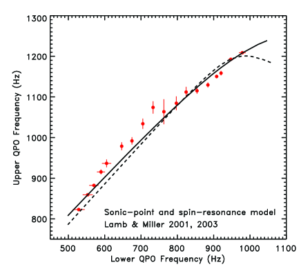
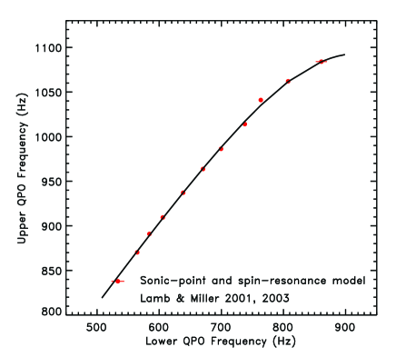
Figure 1 (top panel) displays the fitting result for 4U 1636-53. We set $\nu_{1}\approx\nu_{2}-\nu_{\rm s}/2$ as 4U 1636-53 belongs to the second case in Lamb and Miller (2003). The ratio $\upsilon_{\rm cl}/\upsilon_{\rm g}$ is represented by a free parameter, the torque coefficient $c_{N}$ (see Lamb and Miller, 2001, for detail). Our fitting result is $M=1.545$ $M_{\odot}$, $\nu_{\rm s}=652\pm 5$ Hz, $c_{N}=0.00274$. The fitting does not give a spin frequency close to $581$ Hz. Moreover, our measured $\Delta\nu$ ranges from $220$ to $340$ Hz, which could be smaller or larger than $\nu_{\rm s}/2$ ($290.5$ Hz). In fact, such behavior of $\Delta\nu$ is already shown in Jonker et al (2002). Though successful in explaining a changing $\Delta\nu$ close to half of the spin frequency, the latest version predicts that $\Delta\nu$ is always smaller (larger) than $\nu_{\rm s}/2$ for a prograde (retrograde) flow. When $\nu_{1}$ is below about $800$ Hz, $\Delta\nu$ is larger than $290.5$ Hz; otherwise, it is smaller than $290.5$ Hz. Finally one can notice that the fitting result by fixing $\nu_{\rm s}=581$ Hz shows larger deviations from the data points.

The fitting result for Sco X-1 is shown in Figure 1 (bottom panel), giving $M=1.80$ $M_{\odot}$, $\nu_{\rm s}=329.5$ Hz (or $\nu_{\rm s}=659$ Hz) and $c_{N}=0.00216$, depending on which case we choose. Comparing with the fitting result in Lamb and Miller (2001) and Lamb and Miller (2001), we get a larger $M$ and a slightly smaller $\nu_{\rm s}$. The reduced $\chi^{2}$ is slightly larger, partly due to our more precise results with smaller error bars.

3.2. Comparisons with orbital resonance models

Kluźniak and Abramowicz (2001), Abramowicz et al (2003) introduced several kHz QPO models based on the idea of the resonances between the radial and vertical frequencies in orbital motion.

3.2.1 The $2:3$ parametric resonance model

A parametric resonance instability occurs near $\omega_{r}=2\omega_{\theta}/n$ for $n=1,2,3,\cdots$ in an oscillator that obeys a Mathieu-type equation of motion,

$$\delta\ddot{\theta}+\omega^{2}_{\theta}[1+h\cos(\omega_{r}t)]\delta\theta=0\ ,$$ (3)

where $\delta\theta$ is the small deviation of elevation $\theta$, the dot denotes the time derivative, $h$ is a known constant. $\omega_{r}=2\pi\nu_{r}$ and $\omega_{\theta}=2\pi\nu_{\theta}$, where $\nu_{r}$ and $\nu_{\theta}$ are the radial and vertical epicyclic frequency, respectively (Abramowicz et al, 2003).

The model predicts $\nu_{r}:\nu_{\theta}=2:n$. When $n$ has the smallest possible value, the strongest resonance is excited. Since $\nu_{r}<\nu_{\theta}$, the smallest possible value for resonance is $n=3$ , meaning that $\nu_{r}:\nu_{\theta}=2:3$. Simply supposing $\nu_{1}=\nu_{r}$ and $\nu_{2}=\nu_{\theta}$ (Kluźniak and Abramowicz, 2002), one can infer the $2:3$ ratio of the twin kHz QPO peak frequencies. The excitation of the resonance has been studied with numerical simulations (Abramowicz et al, 2003) and an analytic method (Rebusco, 2004).

Figure 2.— Fitting results to the parametric resonance model for 4U 1636-53 (top) and Sco X-1(bottom). The dashed curve represents the model with $\nu_{1}:\nu_{2}=2:3$. The dotted curves denote the simple assumption ($\nu_{2}=\nu_{\theta}$, $\nu_{1}=\nu_{r}$) with different $M$ and $j$. The solid curve shows a linear frequency relation according to Abramowicz et al (2005).

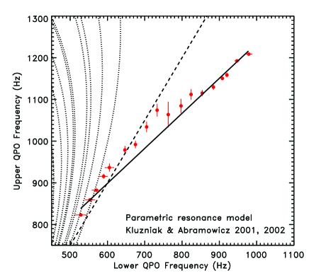
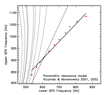
The behavior of the frequency relation in the parametric resonance model is shown in Figure 2, in comparison to our measured data. At first, one can notice that the linear $2:3$ frequency relation (dashed) is not in agreement with the observations. Then we also notice that the model with $\nu_{2}=\nu_{\theta}$ and $\nu_{1}=\nu_{r}$ deviates from data much more (dotted); it is even unable to follow the basic downward-bending track of the data points. Actually the assumption $\nu_{1}=\nu_{r}$ is inappropriate for a NS. Under the condition of $M\in[1.4,2.4]$ $M_{\odot}$ and $j\in[0,0.3]$, theoretical $\nu_{r}$ has a maximum value about $635$ Hz when $M=1.4$ $M_{\odot}$, $j=0.3$ (see e.g. Stella and Vietri, 1999, the equations of orbital frequencies). However, the measured $\nu_{1}$ reaches as large as $800\sim 1000$ Hz. As shown in the figure, the rightmost dotted curve represents the predicted frequency relation with $M=1.4$ $M_{\odot}$, $j=0.3$ and the leftmost one with $M=2.4$ $M_{\odot}$, $j=0$. The predicted curves with other values of $M$ and $j$ lie between them. Finally a linear frequency relation, i.e. $\nu_{2}=\nu_{\theta}$ and $\nu_{2}=k\nu_{1}+b$, is proposed in Abramowicz et al (2005). We use it to fit the data and get $k=0.840$, $b=395$ Hz for 4U 1636-53, and $k=0.805$, $b=422$ Hz for Sco X-1, respectively. Then we get the ratio of $\nu_{1}$ to $\nu_{2}$ for these two sources to be $0.725$ and $0.683$, respectively, close to but higher than $2:3$. Adopting a function as $\nu_{2}=k*\nu_{1}+b$, Belloni et al (2005) also concluded the similar ratios. We will discuss the ratios in Section 4. Here we just show that the linear fit is naturally disfavored by the data points with apparent non-linearity.

3.2.2 The forced $1:2$ and $1:3$ resonance model

In the numerical simulations of oscillations of a perfect fluid torus (Abramowicz et al, 2003), there is an evident resonant forcing of vertical oscillations. The forcing is caused by the radial oscillations through a pressure coupling. This result supports another possible resonance model (Abramowicz and Kluźniak, 2001; Abramowicz et al, 2004). In the model, the resonances occur in a forced non-linear oscillator,

$$\delta\ddot{\theta}+\omega^{2}_{\theta}\delta\theta+[{\rm non\ linear\ terms\ in}\ \delta\theta]=h(r)\cos(\omega_{r}t),\omega_{\theta}=n\omega_{r}$$ (4)

here again $\omega_{r}=2\pi\nu_{r}$ and $\omega_{\theta}=2\pi\nu_{\theta}$.

This model predicts that one of the combination frequencies, i.e. $\nu_{-}=\nu_{\theta}-\nu_{r}$ and $\nu_{+}=\nu_{\theta}+\nu_{r}$, has a $2:3$ ratio to the vertical frequency. For $n=2$, the forced epicyclic resonance $\nu_{r}:\nu_{\theta}=1:2$,

$$\nu_{1}=\nu_{\theta},\qquad\nu_{2}=\nu_{+},$$ (5)

and for $n=3$, the forced epicyclic resonance $\nu_{r}:\nu_{\theta}=1:3$,

$$\nu_{1}=\nu_{-},\qquad\nu_{2}=\nu_{\theta}.$$ (6)

Figure 3.— The fitting results to the forced resonance models for 4U 1636-53 (top) and Sco X-1(bottom). The solid curve and the dashed one show the forced $1:2$ and $1:3$ resonance model, respectively.

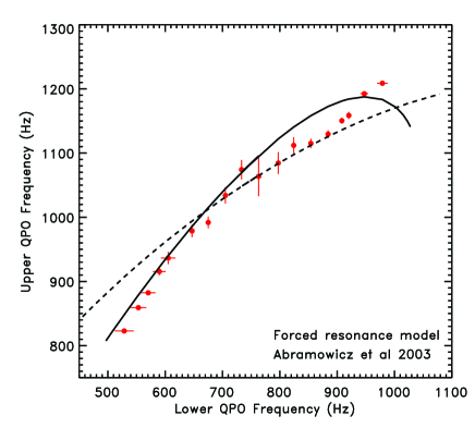
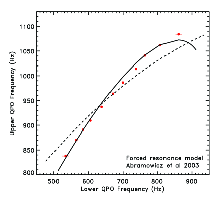
We fit the observed QPO frequency relations with the forced resonance models in Figure 3. The forced $1:2$ model predicts that $\nu_{2}$ climbs up to a maximum value at $\nu_{1}\approx 950$ Hz, then decreases rapidly. However, our analysis results for the two LMXBs do not show the trend that $\nu_{2}$ should decrease as $\nu_{1}$ increases. Regarding the forced $1:3$ model, it cannot adequately describe the data points, especially at the high and low frequencies. The $\nu_{2}$ predicted is higher than that observed at low frequencies, but lower than that observed at high frequencies. It means that the observed $\Delta\nu$ does not decrease so sharply as the model predicts. In addition, these two forced models give very large reduced $\chi^{2}$.

3.3. Comparisons with precession models

This section investigates the predictive ability of three precession models, namely, relativistic precession model, vertical precession model and total precession model. In these precession models, QPOs can be excited by various resonances with the precession frequencies and orbital frequencies under certain conditions, such as inhomogeneities orbiting the inner disk boundary (Stella, 2001).

For the well-known relativistic precession model (Stella and Vietri, 1999), the upper QPO $\nu_{2}$ is assumed to be the azimuthal frequency $\nu_{\phi}$, the lower QPO $\nu_{1}$ is expressed as the relativistic periastron precession frequency,

$$\nu_{1}=\nu_{\phi}-\nu_{r},$$ (7)

$$\nu_{2}=\nu_{\phi}.$$ (8)

In the vertical precession model (Bursa, 2005), $\nu_{1}$ is same as that in Eq. (7); $\nu_{2}$ is hypothesized as $\nu_{\theta}$.

In the total precession model (Stuchlík et al, 2007), $\nu_{1}$ is the total precession frequency, and $\nu_{2}$ is ascribed to the Keplerian frequency $\nu_{\rm K}$ (or the vertical frequency $\nu_{\theta}$),

$$\nu_{1}=\nu_{\theta}-\nu_{r}$$ (9)

$$\nu_{2}=\nu_{\rm K}\qquad or\qquad\nu_{2}=\nu_{\theta}.$$ (10)

Figure 4.— The fitting results to the precession models for 4U 1636-53 (top) and Sco X-1 (bottom). The solid, dotted and dashed curves represent the predictions of the relativistic, vertical and total precession models, respectively. The three curves almost overlap, especially the relativistic and vertical models.

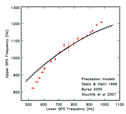
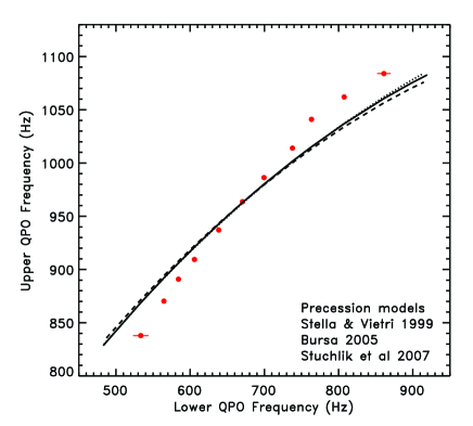
Figure 4 illustrates the comparison of the precession models with the observed data. Notice that the models almost overlap and have the same deviation as the forced $1:3$ resonance model: $\nu_{2}$ is predicted too low at high frequencies and too high at low frequencies. Hence the deviation from the observations increases significantly at high and low frequencies. In addition, the relativistic and vertical precession models give large $M$ and $j$. Though the total precession model give smaller $M$ and $j$, the fit has largest $\chi^{2}$ among the precession models.

3.4. Comparisons with disk oscillation models

The resonances between specific modes in an accretion disk are also studied for exciting the observed kHz QPOs. In this section, we investigate two models of this kind.

3.4.1 The deformed-disk oscillation model

Kato (2001) brought forward the deformed-disk resonance model. kHz QPOs are excited by a horizontal resonance in a deformed (warped or eccentric) disk under inviscid and adiabatic perturbations. The perturbations vary as $\exp[i(\omega t-m\phi)]$, where $\omega$ is the frequency of the perturbations and $m$ ($=0,1,2,\cdots$) denotes the number of arms in the azimuthal direction. Various modes of perturbations are considered in a series of their works (Kato, 2003, 2005, 2009). In the model, QPOs are inertial-acoustic oscillations (p-mode) and the gravity oscillations (g-mode), or their combination. The twin kHz QPOs are,

$$\nu_{1}=2(\nu_{\rm K}-\nu_{r})$$ (11)

$$\nu_{2}=2\nu_{\rm K}-\nu_{r}.$$ (12)

Figure 5.— The fitting results to the deformed-disk resonance model for 4U 1636-53 (top) and Sco X-1(bottom). The solid curve represents the best fitting result with $M\approx 2.4$ $M_{\odot}$, $j=0$. The predicted $M$ and $j$ are almost identical in the two LMXBs.

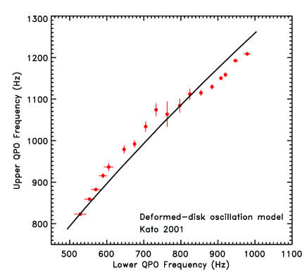
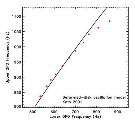
Figure 5 exhibits the best fittings for 4U 1636-53 and Sco X-1. The fitting results ($M\approx 2.4$ $M_{\odot}$, $j=0$) are consistent with that in Kato (2007). The model gives a large NS mass. At the same time, the fittings to the two different NS systems give the same set of $M$ and $j$. However the model describes the measured data points relatively better than most of other models, though it predicts $\nu_{2}$ slightly larger than that observed at high frequencies.

3.4.2 The ‘-1r, -2v’ resonance model

Unlike the deformed disk oscillation model, the perturbations in the ‘-1r, -2v’ resonance model (Török et al, 2007; Bakala et al, 2008) are not stressed in the azimuthal direction. In this model, the kHz QPOs are excited by the resonance between the radial $m=1$ and the vertical $m=2$ modes. The excited QPOs are supposed to be,

$$\nu_{1}=\nu_{\rm K}-\nu_{r},$$ (13)

$$\nu_{2}=2\nu_{\rm K}-\nu_{\theta}.$$ (14)

Figure 6.— The fitting results to the ‘-1r, -2v’ resonance model for 4U 1636-53 (top) and Sco X-1(bottom).

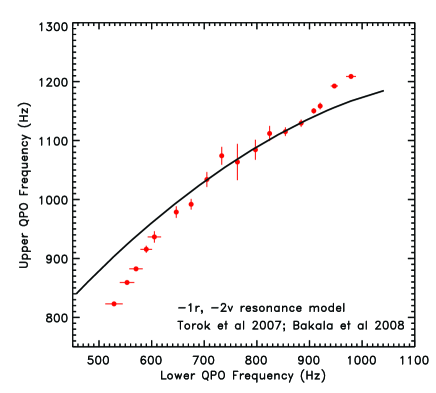
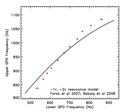
The fitting results to the model are displayed in Figure 6. Like the precession and forced $1:3$ resonance models, the model predictions cannot reproduce the observations, especially at low and high frequencies. The fittings have very large $\chi^{2}$ and give $M=2.4$ $M_{\odot}$ reaching the upper limit in the fitting.

3.5. Comparison with the higher-order nonlinearity model

Mukhopadhyay (2009) treated accreting systems as damped harmonic oscillators. These oscillators exhibit epicyclic oscillations with higher-order nonlinear resonance. The resonance is expected to be driven by the coupling between the strong disturbance from a NS and the weaker one from the flow. In the model, the lower and upper kHz QPOs are proposed to be,

$$\nu_{1}=\nu_{\theta}-\frac{\nu_{\rm s}}{2},$$ (15)

$$\nu_{2}=\nu_{r}+\frac{n}{2}\nu_{\rm s}.$$ (16)

In the disk around a NS, $n=1$ corresponds to a nonlinear coupling, resulting in $\Delta\nu=\nu_{2}-\nu_{1}\sim\nu_{\rm s}/2$; whereas $n=2$ corresponds to a linear coupling, resulting in $\Delta\nu\sim\nu_{\rm s}$. However, $n=3$ may correspond to the higher-order coupling which is expected to be too weak to produce any observable effects. For $n=1$ and $n=2$, the model divides NSs into fast and slow rotators.

To compute the QPO frequencies, the spin parameter $j$ should be determined in the following way. If a NS is considered to be spherical in shape with equatorial radius $R$, spin $\nu_{\rm s}$, mass $M$, radius of gyration $R_{G}$, then the moment of inertia and the spin parameter are computed by,

$$I=MR_{G}^{2},\qquad j=\frac{I\Omega_{s}}{GM^{2}/c},$$ (17)

where $\Omega_{s}=2\pi\nu_{\rm s}$. It is known that for a solid sphere $R_{G}^{2}=2R^{2}/5$ and for a hollow sphere $R_{G}^{2}=2R^{2}/3$. However a very fast rotating NS is expected to be ellipsoidal and not completely solid. Therefore $0.35\leq(R_{G}/R)^{2}\leq 0.5$ is chosen in the model.

Figure 7.— The fitting results to the higher-order nonlinearity model for 4U 1636-53 (top) and Sco X-1(bottom). Top panel: the solid curve represents the best fitting result under $n=1$. The dashed curve, which almost overlaps the solid one, is the fitting under $n=2$. The dotted curve and dot-dashed one denote the fittings by setting $\nu_{\rm s}=581$ Hz under $n=1$ and $n=2$, respectively. Bottom panel: the solid and dashed curves indicate the best fitting results under $n=1$ and $n=2$.

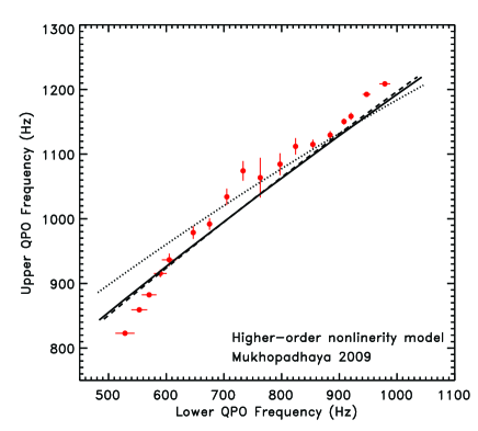
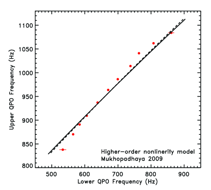
The model parameters, i.e. $M$, $\nu_{\rm s}$, $R$ and $(R_{G}/R)^{2}$, can be obtained by the fitting. For 4U 1636-53, Mukhopadhyay (2009) treated it as a fast rotator with $\nu_{\rm s}=581$ Hz and fit the frequency relation under $n=1$. In his work, only six data points were collected in the diagram of $\Delta\nu$ versus $\nu_{1}$. Then he excluded the data points at low frequencies, corresponding to the ones with large deviations from the model. Finally he gave a low NS mass about $1.2\sim 1.4$ $M_{\odot}$. For Sco X-1, the fitting was done both under $n=1$ and $n=2$ and he argued that Sco X-1 is a slow rotator with $n=2$ and $\nu_{\rm s}$ about $300$ Hz.

Our fitting results with different $n$ are shown in Figure 7. Here we fit all the data points in the two NS systems without any exclusion. For 4U 1636-53, the best fitting value is $M=1.40$ $M_{\odot}$, $\nu_{\rm s}=489$ Hz, $R=23.1$ km, $(R_{G}/R)^{2}=0.38$ under $n=1$ and $M=1.40$, $\nu_{\rm s}=307$ Hz, $R=26.5$ km, $(R_{G}/R)^{2}=0.46$ under $n=2$. We find that under $n=1$ and $n=2$ the model gives the curves almost superposed (solid and dashed in the figure). Moreover, $\nu_{2}$ predicted by the model is too high at low frequencies. By setting $\nu_{\rm s}=581$ Hz and $n=1$, we obtain the results with much larger deviations (dotted curve). For Sco X-1, the model curves under $n=1$ and $n=2$ almost overlap, resulting in $467$ Hz and $294$ Hz spin frequencies. The best fitting value of other parameters is $M=1.40$ $M_{\odot}$, $R=23.0$ km, $(R_{G}/R)^{2}=0.40$ under $n=1$ and $M=1.40$, $R=27.3$ km, $(R_{G}/R)^{2}=0.45$ under $n=2$. For $n=2$, our results are consistent with that in Mukhopadhyay (2009).

3.6. Comparison with the tidal disruption model

Tidal disruption of the orbits of low-mass satellites around a Schwarzschild black hole has recently been studied by Čadež et al (2008). In the clumps of material orbiting such a black hole, a spherical blob can be squeezed and stretched by tidal forces into a ring-like shape along the orbit, and thus making radial oscillations (Germanà et al, 2009). With simulations of such accretion processes, they generated simulated light curves and fit the power spectra of the light curves. Both twin kHz QPOs are found and the peak frequencies are supposed to be,

$$\nu_{1}=\nu_{\rm K},$$ (18)

$$\nu_{2}=\nu_{\rm K}+\nu_{r}.$$ (19)

Figure 8.— The fitting results to the tidal disruption model for 4U 1636-53 (top) and Sco X-1 (bottom). The curves exhibits the disagreement with the data points when $\nu_{1}>800$ Hz.

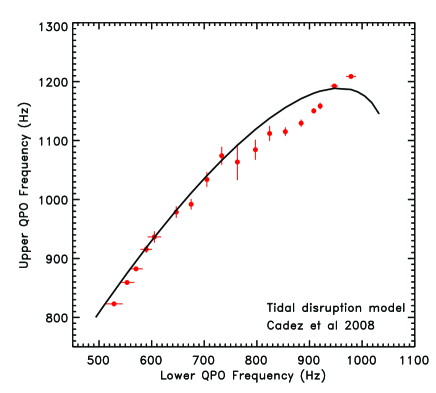
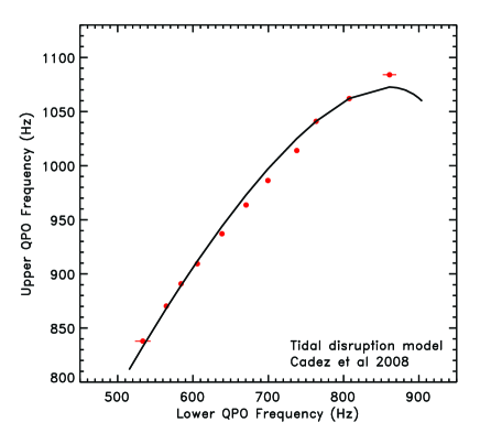
Figure 8 shows the best fittings to this model in the two NS systems. As we see, the model describes well the main parts of the frequency relations, particularly at low frequencies ($\nu_{1}\leq 800$ Hz). At high frequencies, however, the model predicts maximum value of $\nu_{2}$ and then a sharp decrease. It is not supported by observations. Another incompatibility is a high NS mass predicted, which is up to $2.4$ $M_{\odot}$ in this model.

3.7. The Rayleigh-Taylor gravity wave model

Osherovich and Titarchuk (1999) and Titarchuk (2003) described QPOs by the Rayleigh-Taylor instability associated with Rossby waves and rotational splitting. Twin kHz QPOs are explained as oscillations of large scale inhomogeneities (hot blobs) thrown into the NS’s magnetosphere. Participating in the radial oscillations with the Keplerian frequency $\nu_{\rm K}$, such blobs are also simultaneously under the influence of the Coriolis force. For such mode of oscillations, $\nu_{2}$ and $\nu_{\rm K}$ hold an upper hybrid frequency relation: $\nu_{2}^{2}-\nu_{\rm K}^{2}=4\nu_{\rm m}^{2}$, where $\nu_{\rm m}$ is the rotational frequency of the magnetosphere near the equatorial plane. If the magnetosphere corotates with the NS (solid-body rotation), then the spin rotation of the NS would be determined. For the first order approximation, $\nu_{\rm m}=\nu_{\rm s}=const$. Within the second-order approximation, the slow variation of $\nu_{\rm m}$ as a function of $\nu_{\rm K}$ reveals the structure of the magnetospheric differential rotation. Hence, in the model,

$$\nu_{1}=\nu_{\rm K}$$ (20)

$$\nu_{2}=(\nu_{\rm K}^{2}+4\nu_{\rm m}^{2})^{1/2},$$ (21)

and within the dipole-quadrupole-octupole approximation of the magnetic field, the rotation frequency of the magnetosphere is,

$$\nu_{\rm m}(\nu_{\rm K})=C_{0}+C_{1}\nu_{\rm K}^{4/3}+C_{2}\nu_{\rm K}^{8/3}+C_{3}\nu_{\rm K}^{4},$$ (22)

where $C_{0}=\nu_{\rm s}$, $C_{2}=2\sqrt{C_{1}C_{3}}$.

Figure 9.— The fitting results to the Rayleigh-Taylor gravity wave model for 4U 1636-53 (top) and Sco X-1 (bottom). The solid curves are the best fitting results while the dash curve in the top panel is the fitting result by setting $\nu_{\rm s}=581$ Hz.

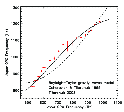
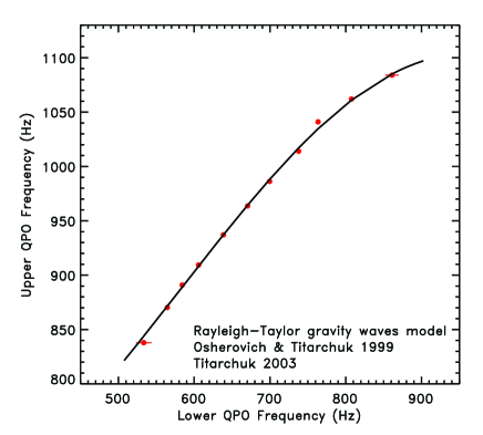
Our fitting treats $M$, $C_{0}$, $C_{1}$, $C_{3}$ as free parameters. The fitting results are shown in Figure 9. For 4U 1636-53, the best fitting (solid curve) returns $M=1.78$ $M_{\odot}$, $C_{0}=371$, $C_{1}=-0.050$, $C_{3}=-7.7$. The spin frequency $\nu_{\rm s}=371$ Hz, not close to $581$ Hz. When we fix $\nu_{\rm s}=581$ Hz, a concave curve (dashed) is obtained, whereas the track of data points bends downward with a convex shape. For Sco X-1, the best fitting values are $M=1.66$ $M_{\odot}$, $C_{0}=350$, $C_{1}=-0.046$, $C_{3}=-10.5$, respectively. Notice that the NS spin frequency of $350$ Hz is consistent with $345$ Hz in Osherovich and Titarchuk (1999). Moreover, the resulting NS mass $1.66$ $M_{\odot}$ is reasonable based on the EOS of NS (Lattimer and Prakash, 2007).

3.8. Comparisons with the models including the effect of magnetohydrodynamics

The last two models above have included the effect of magnetohydrodynamics (MHD) around a rotating NS. In a LMXB containing a magnetized NS, the material in the accretion disk first rotates in a Keplerian motion, then corotates with the magnetosphere as it is trapped by the NS magnetic field at the magnetospheric radius, and finally flows along the field lines to the polar cap of the NS. Some resonant modes may be excited by the perturbations at the magnetospheric radius (Zhang, 2004; Shi and Li, 2009).

3.8.1 The MHD Alfvén wave oscillation model

Zhang (2004) explained the twin kHz QPOs with the MHD Alfvén wave oscillations excited by the distortion of the NS magnetosphere. The model assumes that the infalling MHD material of the Keplerian accretion flow distorts the magnetosphere in the regions with enhanced mass density gradients, leading to resonant shear Alfvén waves. In this model, the upper frequency QPO is the Keplerian orbital frequency,

$$\nu_{2}=\nu_{\rm K}=1850AX^{3/2}\quad{\rm Hz},$$ (23)

with the parameters $X=R/r$ and $A=(m/R_{6}^{3})^{1/2}$, where $R_{6}=R/10^{6}$ $({\rm cm})$ and $m=M/M_{\odot}$ are the NS radius $R$ and mass $M$ in units of $10^{6}$ cm and solar masses, respectively. The quantity $A^{2}$ is proportional to the average mass density of the NS, expressed as, $\langle{\rho}\rangle=3M/(4\pi{R^{3}})\approx{2.4}\times 10^{14}({\rm g}/{\rm cm}^{3})(A/0.7)^{2}$.

The lower frequency QPO is identified as the Alfvén oscillation frequency, given as,

$$\nu_{1}=\nu_{2}X^{3/4}\sqrt{1-\sqrt{1-X}}.$$ (24)

Figure 10.— The fitting results to the MHD Alfvén wave model for 4U 1636-53 (top) and Sco X-1(bottom).

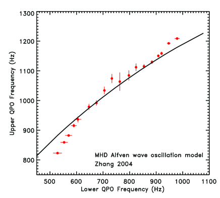
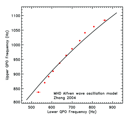
Since $X$ is eliminated in the fitting process, we only have one parameter $A$. The comparisons between the model predictions and the observations are shown in Figure 10. Similar to the precession models, this model also predicts $\nu_{2}$ too high at low frequencies and too low at high frequencies, leading to the increased deviations from the observations at low and high frequencies. The result also indicates that $\Delta\nu$ predicted by this model decreases too sharply compared to the observations. The fitting for Sco X-1 is somewhat better than that for 4U 1636-53. Our result of $A\approx 0.7$ agrees with that obtained by Zhang et al (2008), in which the relation of $\Delta\nu$ versus $\nu_{2}$ was fitted and the result shows a discrepancy with the observations.

3.8.2 The MHD model

Shi and Li (2009) presented another explanation for kHz QPO signals in LMXBs based on MHD oscillation modes in a NS’s magnetosphere. Several MHD wave modes are derived by solving the dispersion equations. They proposed that the coupling of the two resonant MHD modes may lead to the twin kHz QPOs. Finally, they presented the following linear frequency relations,

$$\nu_{2}=\sqrt{1+\delta^{2}}(\nu_{1}+\nu_{\rm s}),\qquad({\rm LSCS})$$ (25)

$$\nu_{2}=\frac{1}{\sqrt{1+\varepsilon^{2}}}(\nu_{1}+\nu_{\rm s}),\qquad({\rm SSCS})$$ (26)

where $\delta^{2}=(\lambda^{2}-\eta^{2})/(1+\eta^{2})$ and $\varepsilon^{2}=(\eta^{2}-\lambda^{2})/(1+\lambda^{2})$. Here $\lambda$ and $\eta$ are two constants linking the Alfvén velocity, acoustic velocity and Keplerian velocity of MHD wave in the model. The model divided the twin kHz QPOs into two groups with the slope of $\nu_{2}/\nu_{\rm s}$ vs. $\nu_{1}/\nu_{\rm s}$ relation either larger or smaller than 1.0, i.e., the large slope coefficient sources (LSCS) and the small slope coefficient sources (SSCS), respectively. With our fitting, we find that both 4U 1636-53 and Sco X-1 belong to the latter group, since Eq. (25) gives bad fitting results with reduced $\chi^{2}>10^{5}$.

Figure 11.— The fitting results to the MHD model for 4U 1636-53 (top) and Sco X-1(bottom). The solid curves are the best fitting results. In the top panel, the dashed curve is the result with $\nu_{\rm s}=581$ Hz fixed.

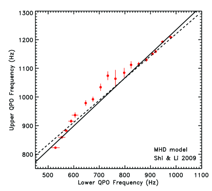
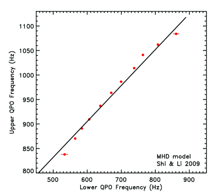
The fitting results are plotted in Figure 11. Firstly, both for 4U 1636-53 and Sco X-1, the observed relations of $\nu_{2}$ with $\nu_{1}$ are not linear; the data points have a track to bend downwards. Secondly, for 4U 1636-53, the best fitting predicts $\epsilon=0.65$ and $\nu_{\rm s}=470$ Hz. The spin frequency is not close to $581$ Hz. Also, Shi and Li (2009) cannot fit well 4U 1636-53 by holding $\nu_{\rm s}=581$ Hz. Their result gives $\epsilon=0.77$ and a large reduced $\chi^{2}=23$. In the case of Sco X-1, our fitting gives $\nu_{\rm s}=525$ Hz, considerably larger than that from other models.

4. Discussion and conclusion

We have presented the newly obtained and more accurate results on the frequency relations of the kHz twin QPOs for 4U 1636-53 and Sco X-1. The peak frequencies of lower and upper QPOs are almost directly proportional to each other. The data points tend to bend downwards between $500$ to $1250$ Hz in the diagram of $\nu_{1}$ versus $\nu_{2}$. Both of the frequency relations show some subtle structure around $\nu_{1}\approx 800$ Hz.

Based on the frequency relations, we have systematically investigated the predictive ability of all currently available models, with which the frequency relation can be calculated. Our conclusions are as follows:

(1) The sonic-point and spin-resonance model seems to be only suitable for Z-sources. The model describes well the frequency relation for Sco X-1. However, in the case of 4U 1636-53, the model predicts that $\Delta\nu$ is always less than half of the spin frequency for a prograde flow, while the observed $\Delta\nu$ can be larger and smaller than $\nu_{\rm s}/2$. It indicates that a single rotational direction of accretion flow cannot explain the behavior of $\Delta\nu$. According to the model, such behavior of $\Delta\nu$ may be produced by a flow that retrogrades when it is far away from the NS, but then switches to a prograde orbit at some special radius when it is closer to the NS. However no evidence is found to support such sudden switch of the orbital motion.

(2) The $2:3$ parametric resonance model predicts a frequency relation bending upwards. Within the limit of NS parameters for reasonable NS EOS, it cannot give $\nu_{1}$ as high as observations. Further more, as claimed in previous papers (Belloni et al, 2005; Zhang et al, 2006), this model leads to the predicted $\Delta\nu$ increase with the QPO frequency. However, the observed downward-bending track in the diagram of $\nu_{1}$ versus $\nu_{2}$ indicates a rough inverse proportion between $\Delta\nu$ and $\nu_{1}$ (or $\nu_{2}$). As regards the forced resonance model, the $1:2$ model predicts a decrease of $\nu_{2}$ at high frequencies; the $1:3$ model predicts $\nu_{2}$ higher (lower) than the observed values at low (high) frequencies. In fact, all of the orbital resonance models are introduced to explain the observed clustering of $2:3$ ratios between $\nu_{1}$ and $\nu_{2}$. However, Belloni et al (2005) have demonstrated that a simple random walk of the QPO frequencies can reproduce qualitatively the observed distributions in frequency and frequency ratio. Later Boutelier et al (2009b) have pointed out that the clustering originates naturally from the sensitivity-limited observations and does not support preferred frequency ratios in NS systems. Our results therefore suggest that the orbital resonance models should be further investigated in order to improve their predictive power for the frequency relation.

(3) All the precession models nearly overlap with each other. Their predicted $\nu_{2}$ is higher (lower) than that observed at low (high) frequencies. The deviations from the observations increases significantly at high and low frequencies. In more detail, the relativistic and vertical precession models predict a NS mass higher than $\sim 2.2$ $M_{\odot}$. As can be found from Table 3, when we relax the fitting limits of $M\in[1.4,2.4]$ and $j\in[0,0.3]$, the extended analysis shows that these two models could describe the data points better with relatively higher $M$ and $j$. Essentially, the inferred high NS mass may be arisen from the assumption of the vacuum circumstance around the NS in introducing the periastron precession term (Zhang et al, 2009). It should be mentioned that considering a small eccentricity ($\lesssim 0.1$) which decreases with increasing $\nu_{\phi}$, the relativistic precession model would explain the frequency relation better (Stella and Vietri 1999). In this paper, we do not consider the effect of eccentricity on the frequency relation because we focus on the NS properties. For the total precession model, it gives lower values of $M$ and $j$ but larger reduced $\chi^{2}$.

(4) The deformed-disk resonance model describes the observations relatively better than most of models. The fittings give the same $M$ and $j$ for the two LMXBs. It suggests that the model may reveal some common properties of Atoll and Z sources. Nevertheless the high mass predicted and the deviations at high frequencies show the model could be modified. For example, the effect of magnetic field could be taken into account. For the ‘-1r, -2v’ resonance model, it behaves like the procession models. Considering that the best fitting results of these two models approach the upper limit of $M$, we also performed the extended fitting. Both for 4U 1636-53 and Sco X-1, the fitting results do not improve significantly.

(5) The higher-order nonlinearity model classifies NSs based on the values of $n$. After the investigation, one can notice that the model predict the nearly identical frequency relations under all values of $n$ taken here. Thereby, given that we do not know the spin frequency of Sco X-1, the classification that Sco X-1 is a slow rotator with $n=2$ is not well founded. The superposed fitting curves under $n=1$ and $n=2$ for 4U 1636-53 also indicate some kinds of ambiguity of the classification. Apart from that, when $n=1$ is chosen, like that in Mukhopadhyay (2009), the spin frequency predicted is not close to $581$ Hz. Besides, the model predicts a very low NS mass reaching the lower limit in our fitting. Our extended analysis shows that the NS masses for the two sources are predicted down to $1.0$ $M_{\odot}$, quite low for most known NS EOS.

(6) The tidal disruption model can describe the main part of the observed frequency relations, though it predicts a high NS mass. Maybe it is due to the essential difference between NS and black hole systems. This implies that the kHz QPOs should be greatly affected by the surroundings close to the central object. After all, the agreement with the observations at low frequencies is remarkable, corresponding to the place relatively distant to the center. At that place, the clumps of material (or particles) are not being exposed to the compact object so much. As can be found from Table 3, the fitting results of the model can be improved greatly in our extended fitting, in favor of very large NS masses. The model should be modified to better describe the data points at high frequencies and to get a more reasonable mass for NS.

(7) The Rayleigh-Taylor gravity wave model can follow the frequency relation in Sco X-1, while for 4U 1636-53 it cannot predict the $581$ Hz spin frequency. This may be because the dipole-quadrupole-octupole approximation is not sufficiently accurate for the magnetic field. Therefore, this model seems promising for explaining the origin of kHz QPOs if its description of NS magnetic field is more accurate. For the sake of comprehensiveness, it should be noted that this model predicts not only the high-frequency QPOs, but also the low frequency ones. When the low QPOs are also considered, the fittings do not always work, unless for one particular frequency range one of the low-frequency QPOs is assumed to be a harmonic of an unseen one, whereas in the other intervals it is the fundamental frequency.

(8) The MHD Alfvén wave oscillation model has the same problem as the precession models with increased deviations from the observations at high and low frequencies. It should be noted that the model was put forward based on the analogy of the solar coronal atmosphere to a NS system. Though the solar coronal atmosphere has been studied a lot, the mechanism of Alfvén wave oscillations in a NS system remains unclear. The model’s performance in our fittings indicates that such mechanism should be investigated further.

(9) The MHD model predicts a linear frequency relation, which is inconsistent with the measured frequency relations. At the same time, the model cannot predict reasonable spin frequencies for the two NSs.

Generally, we also find that:

(10) These models diverge strongly in their predictions of the NS properties. Different models predict spin frequency from less than $300$ Hz to more than $600$ Hz. The angular momentum is predicted as from 0 to 0.3, covering entirely the range of the limit in the fitting. The predicted NS mass from different models also covers the whole range $[1.4,2.4]$ $M_{\odot}$.

(11) The problem of increased deviations at high and low frequencies exists in six models: the forced $1:3$ model, the three precession models, the ‘-1r, -2v’ resonance model and the MHD Alfvén wave oscillation model. The first five models almost overlap in the plot of their fitting results. Since $\nu_{\rm K}\approx\nu_{\theta}$ (exactly equal if $\nu_{\rm s}=0$), these five models have nearly identical expressions of $\nu_{1}$ and $\nu_{2}$. Those five models form the group of the largest $\chi^{2}$ in Table 2. The MHD Alfvén oscillation model performs slightly better than those five models, despite that its $\chi^{2}$ remains much larger than the other remaining models. All of the six models propose that the upper frequency QPO is Keplerian, i.e. $\nu_{2}=\nu_{\rm K}$. It infers that for these models, the interpretation is not favored by the data.

(12) Those models including the effects of magnetic field obtain the best fitting results, such as the sonic-point beat frequency and the Rayleigh-Taylor gravity wave model. At least, they can depict the frequency relation for Sco X-1.

Finally, one should notice the fact that no model gives a statistically acceptable $\chi^{2}$ in the fittings. We argue that all the models predicting a linear, power-law or any other frequency relation are not fully supported by the observations, at least for this two sources.

After the investigation, we comment that since among these models we investigated here, three models of them (deformed-disk resonance, tidal disruption and the Rayleigh-Taylor gravity wave model) have performed relatively better than other models, we speculate that a model which combines these three models together could reveal the physical origin of the observed kHz QPO signals. It is worth noticing that each of them still has its own problems.

Table 2The fitting parameters of all models for 4U 1636-536 and Sco X-1. The errors have been computed by setting $\Delta\chi^{2}=1$.

	4U 1636-536				Sco X-1
Models	M ($M_{\odot}$)	j or spin (Hz)	Reduced $\chi^{2}$	Dof	M ($M_{\odot}$)	j or spin (Hz)	Reduced $\chi^{2}$	Dof
SP SR Case 1	-	-	-	-	1.80$\pm$0.02	330$+2\atop-1$	3.0	8
SP SR Case 2	1.545$+0.046\atop-0.042$	652$\pm$6	7.5	15	1.80$\pm$0.02	659$+4\atop-2$	3.0	8
fix spin	1.746$+0.008\atop-0.009$	581	$18.9$	15
Para. Res.	great	departure	from	frequency	relation
linear relation	2.04$\pm$0.01	0.19$\pm$0.01	11	14	2.09$\pm$0.01	0.07$\pm$0.01	71	7
Forced 1:3	1.815$+0.003\atop-0.004$	0.0001$+0.0010\atop-0.0001$	186	16	1.97$\pm$0.01	0.000$+0.001\atop-0.0$	306	9
Forced 1:2	2.095$+0.006\atop-0.003$	0.0$+0.005\atop-0.0$	28	16	2.32$\pm$0.01	0.0$+0.001\atop-0.0$	54	9
Rel. Pre.	2.319$+0.003\atop-0.005$	0.30$+0.0\atop-0.001$	156	16	2.40$+0.0\atop-0.01$	0.250$\pm$0.001	244	9
Ver. Pre.	2.160$+0.003\atop-0.004$	0.300$+0.0\atop-0.001$	158	16	2.33$\pm$0.01	0.299$\pm$0.001	230	9
Tot. Pre.	1.814$+0.004\atop-0.003$	0.0$+0.001\atop-0.0$	186	16	1.971$+0.001\atop-0.002$	0.0$+0.001\atop-0.0$	306	9
Deformed-disk	2.400$+0.0\atop-0.001$	0.00$+0.0002\atop-0.0$	31	16	2.400$+0.0\atop-0.001$	0.0$+0.001\atop-0.0$	447	9
‘-1r, -2v’ Res.	2.400$+0.0\atop-0.001$	0.238$+0.002\atop-0.001$	154	16	2.400$+0.0\atop-0.002$	0.172$+0.002\atop-0.001$	248	9
Hi. non-line. n=1	1.401$\pm 0.001$	488.6$+0.01\atop-0.07$	85	14	1.40$+0.01\atop-0.0$	467 $\pm$1	86	7
fix spin	2.10$+0.01\atop-0.02$	581	211	15
Hi. non-line. n=2	1.401$\pm 0.001$	306.7$+0.01\atop-0.07$	70	14	1.40$+0.01\atop-0.0$	294$\pm$1	70	7
Tidal Disruption	2.400$+0.0\atop-0.003$	0.166$+0.001\atop-0.002$	18	16	2.400$+0.0\atop-0.002$	0.045$+0.001\atop-0.002$	43	9
R-T G. Wave	1.78$+0.47\atop-0.38$	371.1$+1.2\atop-2.7$	10	14	1.66$+0.34\atop-0.26$	350.4$+0.3\atop-0.8$	4.4	7
fix spin	1.86$+0.38\atop-0.40$	581	$38$	15
Alfvén Wave Res.	A=0.699$\pm$0.002		81	17	A=0.658$\pm$0.001		68	10
MHD	$\epsilon=$0.647$+0.013\atop-0.014$	470.3$+7.3\atop-7.7$	10	16	$\epsilon$=0.928$+0.001\atop-0.007$	635$+6\atop-5$	56	9
fix spin	$\epsilon$=0.928$+0.002\atop-0.003$	581	21	17

Table 3The fitting parameters of the extended analysis for 4U 1636-536 and Sco X-1.

	4U 1636-536				Sco X-1
Models	M ($M_{\odot}$)	j or spin (Hz)	Reduced $\chi^{2}$	Dof	M ($M_{\odot}$)	j or spin (Hz)	Reduced $\chi^{2}$	Dof
Rel. Pre.	2.8	0.49	131	16	3.07	0.499	165	9
Ver. Pre.	2.46	0.5	141	16	2.65	0.5	188	9
Deformed-disk	2.48	0.00	22	16	2.45	0.0	395	9
‘-1r, -2v’ Res.	3.61	0.500	129	16	3.75	0.471	183	9
Hi. non-line. n=1	1.0	460	50	14	1.0	438	61	7
Hi. non-line. n=2	1.0	283	34	14	1.0	282	59	7
Tidal Disruption	3.33	0.483	8	16	2.70	0.19	26	9

References

- Abramowicz et al (2003) Abramowicz M.A., Karas V., Kluźniak W., Lee W.H., Rebusco P., PASJ, 55, 467 (2003)
- Abramowicz et al (2004) Abramowicz M.A., Kluźniak W., Stuchlik K., Török G., arXiv:astro-ph/0401464 (2004)
- Abramowicz et al (2005) Abramowicz M.A., Barret D., Bursa M., Horák J., Kluźniak W., Rebusco P., Török G., ragt.meet, 1 (2005)
- Abramowicz and Kluźniak (2001) Abramowicz M.A. and Kluźniak W., A&A, 374, L19 (2001)
- Bachetti et al (2010) Bachetti M., Romanova M., Kulkarni A., Burderi L., di Salvo T., MNRAS, 403, 1193 (2010)
- Bakala et al (2008) Bakala, P., Šrámková E., Stuchlík Z., Török G., AIPC, 1054, 123 (2008)
- Barret et al (2005) Barret D., Olive J.F., Miller M.C., MNRAS, 361, 855 (2005)
- Barret et al (2006) Barret D., Olive J.F., Miller M.C., MNRAS, 370, 1140 (2006)
- Belloni et al (2005) Belloni T., Méndez M., Homan J., ESNS.Conf., 339 (2005)
- Boutelier et al (2009a) Boutelier M., Barret, D., Miller M.C., MNRAS, 399, 1901 (2009)
- Boutelier et al (2009b) Boutelier M., Barret, D., Lin Y.F., Török G., MNRAS, 401, 1290 (2010)
- Bursa (2005) Bursa M., RAGtime 6/7: Workshops on black holes and neutron stars, 39 (2005)
- Čadež et al (2008) Čadež A., Calvani M., Kostić U., A&A, 478, 527 (2008)
- Germanà et al (2009) Germanà C., Kostić U., Čadež A., Calvani M., AIPC, 1126, 367 (2009)
- Jonker et al (2002) Jonker P.G., Méndez M. and van der Klis M., MNRAS, 336, L1 (2002)
- Kato (2001) Kato S., PASJ, 53, 1 (2001)
- Kato (2003) Kato S., PASJ, 55, 801 (2003)
- Kato (2005) Kato S., PASJ, 57, 699 (2005)
- Kato (2007) Kato S., PASJ, 59, 451 (2007)
- Kato (2009) Kato S., PASJ, 61, 1237 (2009)
- Kluźniak and Abramowicz (2001) Kluźniak W. and Abramowicz M.A., Acta Physica Polonica B, 32, 3605(2001)
- Kluźniak and Abramowicz (2002) Kluźniak W. and Abramowicz M.A., arXiv:astro-ph/0203314 (2002)
- Lamb and Miller (2001) Lamb F.K. and Miller M.C., ApJ, 554, 1210 (2001)
- Lamb and Miller (2003) Lamb F.K. and Miller M.C., arXiv:astro-ph/0308179 (2003)
- Lattimer and Prakash (2007) Lattimer J.M., Prakash M., Physics Reports, 442, 109 (2007)
- Méndez and van der Klis (2000) Méndez M. and van der Klis M., MNRAS, 318, 938 (2000)
- Méndez et al (1998) Méndez M., van der Klis M., van Paradijs J., Lewin W.H.G., Vaughan B.A., Kuulkers E., Zhang W., Lamb F.K., Psaltis D., ApJ, 494, L65 (2000)
- Miller et al (1998) Miller M.C., Lamb F.K., Psaltis D., ApJ, 508, 791 (1998)
- Mukhopadhyay (2009) Mukhopadhyay B., ApJ, 694, 387 (2009)
- Osherovich and Titarchuk (1999) Osherovich V. and Titarchuk L., ApJ, 522, L113 (1999)
- Rebusco (2004) Rebusco P., PASJ, 56, 553 (2004)
- Shi and Li (2009) Shi C. and Li X.D., MNRAS, 392, 264 (2009)
- Stella and Vietri (1999) Stella L. and Vietri M., Physical Review Letters, 82, 17 (1999)
- Stella (2001) Stella L., AIPC, 599, 365 (2001)
- Strohmayer (2001) Strohmayer T.E., Advances in Space Research, 28, 511 (2001)
- Strohmayer and Markwardt (2002) Strohmayer T.E. and Markwardt C.B., ApJ, 577, 337 (2002)
- Stuchlík et al (2007) Stuchlík Z., Török G., Bakala P., arXiv:0704.2318 (2007)
- Titarchuk (2003) Titarchuk L., ApJ, 591, 354 (2003)
- Török et al (2007) Török G., Bursa M., Horák J., Stuchlík Z., Bakala P., ragt.meet, 501 (2007)
- van der Klis (2006) van der Klis M., Advances in Space Research, 38, 2675 (2006)
- Zhang (2004) Zhang C.M., A&A, 423, 401 (2004)
- Zhang et al (2006) Zhang C.M., Yin H.X., Zhao Y.H., Song L.M., Zhang F., MNRAS, 366, 1373 (2006)
- Zhang et al (2008) Zhang C.M., Yin H.X., Zhao Y.H., AIPC, 968, 223 (2008)
- Zhang et al (2009) Zhang C.M., Wei Y.C., Yin H.X., Zhao Y.H., Lei Y.J., Song L.M., Zhang F., Yan Y., arXiv:0912.0768 (2009)