Two-loop Resummation in Fractional Analytic Perturbation Theory

Alexander P. Bakuleva111E-mail: bakulev@theor.jinr.ru
a Bogoliubov Laboratory of Theoretical Physics, JINR
Jolio-Curie 6, Dubna, 141980 Russia
Abstract

This talk describes the resummation approach in (Fractional) Analytic Perturbation Theory (FAPT) in QCD. First, we make a short historical review of the (F)APT approach and then shortly describe the global scheme of FAPT which allows one to take into account heavy-quark thresholds. After that we show how it is possible to resum a non-power series in (F)APT both in the one- and two-loop approximations. As an application we suggest our analysis of the Higgs boson decay H0bb¯superscript𝐻0𝑏¯𝑏{H^{0}\to b\overline{b}}, important for the LHC program, and of the vector-current Adler function.

1 Analytic Perturbation Theory in QCD

First, I’d like to remind the history of Analytic Perturbation Theory (APT). Strictly speaking, APT was initiated by the paper of N. N. Bogolyuov et al. in 1959 [1], where ghost-free effective coupling for QED was constructed using the dispersion-relations method. Then, in 1982, Radyushkin [2], and Krasnikov and Pivovarov [3], using the same dispersion-relations technique, suggested regular (for sΛ2𝑠superscriptΛ2s\geq\Lambda^{2}) QCD running coupling in the Minkowski region, αs(s)as(s)/βfsubscript𝛼𝑠𝑠subscript𝑎𝑠𝑠subscript𝛽𝑓\alpha_{s}(s)\equiv a_{s}(s)/\beta_{f}, namely, as[L]=π1arctan(π/L)subscript𝑎𝑠delimited-[]𝐿superscript𝜋1𝜋𝐿a_{s}[L]=\pi^{-1}\arctan(\pi/L) with L=ln(s/Λ2)𝐿𝑠superscriptΛ2L=\ln(s/\Lambda^{2}) and βf=b0(Nf)/(4π)=(112Nf/3)/(4π)subscript𝛽𝑓subscript𝑏0subscript𝑁𝑓4𝜋112subscript𝑁𝑓34𝜋\beta_{f}=b_{0}(N_{f})/(4\pi)=(11-2N_{f}/3)/(4\pi).222We use the notations f(Q2)𝑓superscript𝑄2f(Q^{2}) and f[L]𝑓delimited-[]𝐿f[L] in order to specify the arguments we mean — squared momentum Q2superscript𝑄2Q^{2} or its logarithm L=ln(s/Λ2)𝐿𝑠superscriptΛ2L=\ln(s/\Lambda^{2}) or ln(Q2/Λ2)superscript𝑄2superscriptΛ2\ln(Q^{2}/\Lambda^{2}), that is f[L]=f(Λ2eL)𝑓delimited-[]𝐿𝑓superscriptΛ2superscript𝑒𝐿f[L]=f(\Lambda^{2}\cdot e^{L}) and Λ2superscriptΛ2\Lambda^{2} is usually referred to the Nf=3subscript𝑁𝑓3N_{f}=3 region. (This normalized coupling as[L]subscript𝑎𝑠delimited-[]𝐿a_{s}[L] in standard QCD PT is just 1/L1𝐿1/L in the one-loop approximation.)

Thirteen years later, Dokshitzer et al. constructed an IR finite αseff(Q2)superscriptsubscript𝛼𝑠effsuperscript𝑄2{\alpha_{s}^{\textbf{eff}}(Q^{2})} in the Euclidean domain using a renormalon-based approach with dispersion relations [4]. After that, Jones and Solovtsov [5, 6] discovered the coupling which appears to be finite for all s𝑠s and coincides with the Radyushkin’s one for sΛ2𝑠superscriptΛ2s\geq\Lambda^{2}, namely

𝔄1[L]subscript𝔄1delimited-[]𝐿\displaystyle{\mathfrak{A}}_{1}[L]\!\! =\displaystyle\!\!=\!\! sρ1(σ)σ𝑑σ=1πarccosLπ2+L2.superscriptsubscript𝑠subscript𝜌1𝜎𝜎differential-d𝜎1𝜋𝐿superscript𝜋2superscript𝐿2\displaystyle\!\!\int_{s}^{\infty}\!\frac{\rho_{1}(\sigma)}{\sigma}\,d\sigma\ =\ \frac{1}{\pi}\,\arccos\frac{L}{\sqrt{\pi^{2}+L^{2}}}\,. (1a)
Just at the same time, Ball, Beneke and Braun reproduced in the pQCD-based renormalon approach as[L]=π1arctan(π/L)subscript𝑎𝑠delimited-[]𝐿superscript𝜋1𝜋𝐿a_{s}[L]=\pi^{-1}\arctan(\pi/L) in the low-energy Minkowski region [7, 8], and Shirkov and Solovtsov [9], using the same dispersion-relations approach of [1], discovered the ghost-free coupling,
𝒜1[L]subscript𝒜1delimited-[]𝐿\displaystyle\mathcal{A}_{1}[L]\!\! =\displaystyle\!\!=\!\! 0ρ1(σ)σ+Q2𝑑σ=1L1eL1,superscriptsubscript0subscript𝜌1𝜎𝜎superscript𝑄2differential-d𝜎1𝐿1superscript𝑒𝐿1\displaystyle\!\!\int_{0}^{\infty}\!\frac{\rho_{1}(\sigma)}{\sigma+Q^{2}}\,d\sigma\ =\ \frac{1}{L}-\frac{1}{e^{L}-1}\,, (1b)

in the Euclidean region with L=ln(Q2/Λ2)𝐿superscript𝑄2superscriptΛ2L=\ln(Q^{2}/\Lambda^{2}). But Shirkov–Solovtsov approach, named APT, appears to be more powerful: in the Euclidean domain, q2=Q2superscript𝑞2superscript𝑄2\displaystyle-q^{2}=Q^{2}, L=lnQ2/Λ2𝐿superscript𝑄2superscriptΛ2\displaystyle L=\ln Q^{2}/\Lambda^{2}, it generates the set of images for the effective coupling and its n𝑛n-th powers, {𝒜n[L]}nsubscriptsubscript𝒜𝑛delimited-[]𝐿𝑛\displaystyle\left\{{\mathcal{A}}_{n}[L]\right\}_{n\in\mathbb{N}}, whereas in the Minkowski domain, q2=ssuperscript𝑞2𝑠\displaystyle q^{2}=s, L=lns/Λ2𝐿𝑠superscriptΛ2\displaystyle L=\ln s/\Lambda^{2}, it generates another set, {𝔄n[L]}nsubscriptsubscript𝔄𝑛delimited-[]𝐿𝑛\displaystyle\left\{{\mathfrak{A}}_{n}[L]\right\}_{n\in\mathbb{N}} (see also in [10]). APT is based on the Renormalization Group (RG) and causality that guarantees standard perturbative UV asymptotics and spectral properties. The power series mdmasm[L]subscript𝑚subscript𝑑𝑚superscriptsubscript𝑎𝑠𝑚delimited-[]𝐿\sum_{m}d_{m}a_{s}^{m}[L] transforms into a non-power series mdm𝔄m[L]subscript𝑚subscript𝑑𝑚subscript𝔄𝑚delimited-[]𝐿\sum_{m}d_{m}{\mathfrak{A}}_{m}[L] or mdm𝒜m[L]subscript𝑚subscript𝑑𝑚subscript𝒜𝑚delimited-[]𝐿\sum_{m}d_{m}{\mathcal{A}}_{m}[L] in APT. The global version of APT, which takes into account the heavy-quark thresholds, has been elaborated in [11].

By the analytization in APT for an observable f(Q2)𝑓superscript𝑄2f(Q^{2}) we mean the “Källen–Lehmann” representation

[f(Q2)]an=0ρf(σ)σ+Q2iϵ𝑑σsubscriptdelimited-[]𝑓superscript𝑄2ansuperscriptsubscript0subscript𝜌𝑓𝜎𝜎superscript𝑄2𝑖italic-ϵdifferential-d𝜎\displaystyle\left[f(Q^{2})\right]_{\text{an}}=\int_{0}^{\infty}\!\frac{\rho_{f}(\sigma)}{\sigma+Q^{2}-i\epsilon}\,d\sigma (2a)
with ρf(σ)=1πIm[f(σ)]subscript𝜌𝑓𝜎1𝜋Imdelimited-[]𝑓𝜎\displaystyle\rho_{f}(\sigma)=\frac{1}{\pi}\,\textbf{Im}\,\big{[}f(-\sigma)\big{]}, which transforms to different prescriptions for couplings in the Euclidean and Minkowski domains
𝒜n[L]subscript𝒜𝑛delimited-[]𝐿\displaystyle\mathcal{A}_{n}[L]\! =\displaystyle\!=\! AE[αsn]=0ρn(σ)σ+Q2𝑑σ;subscriptAEdelimited-[]superscriptsubscript𝛼𝑠𝑛superscriptsubscript0subscript𝜌𝑛𝜎𝜎superscript𝑄2differential-d𝜎\displaystyle\!\textbf{A}_{\textbf{E}}\left[\alpha_{s}^{n}\right]=\int_{0}^{\infty}\!\frac{\rho_{n}(\sigma)}{\sigma+Q^{2}}\,d\sigma\,; (2b)
𝔄n[L]subscript𝔄𝑛delimited-[]𝐿\displaystyle\mathfrak{A}_{n}[L]\! =\displaystyle\!=\! AM[αsn]=sρn(σ)σ𝑑σ.subscriptAMdelimited-[]superscriptsubscript𝛼𝑠𝑛superscriptsubscript𝑠subscript𝜌𝑛𝜎𝜎differential-d𝜎\displaystyle\!\textbf{A}_{\textbf{M}}\left[\alpha_{s}^{n}\right]=\int_{s}^{\infty}\!\frac{\rho_{n}(\sigma)}{\sigma}\,d\sigma\,. (2c)

In the one-loop approximation, we have then ρ1(σ)=1/Lσ2+π2subscript𝜌1𝜎1superscriptsubscript𝐿𝜎2superscript𝜋2\rho_{1}(\sigma)=1/\sqrt{L_{\sigma}^{2}+\pi^{2}} and Eqs. (1), whereas analytic images of the higher powers (n2,nformulae-sequence𝑛2𝑛n\geq 2,n\in\mathbb{N}) are [2, BRS00]

(𝒜n[L]𝔄n[L])=1(n1)!(ddL)n1(𝒜1[L]𝔄1[L]).binomialsubscript𝒜𝑛delimited-[]𝐿subscript𝔄𝑛delimited-[]𝐿1𝑛1superscript𝑑𝑑𝐿𝑛1binomialsubscript𝒜1delimited-[]𝐿subscript𝔄1delimited-[]𝐿\displaystyle{\mathcal{A}_{n}[L]\choose\mathfrak{A}_{n}[L]}=\frac{1}{(n-1)!}\left(-\frac{d}{dL}\right)^{n-1}{\mathcal{A}_{1}[L]\choose\mathfrak{A}_{1}[L]}\,. (3)

At first glance, the APT is a complete theory supplying tools to produce an analytic answer for any perturbative series in QCD. But in 2001 Karanikas and Stefanis reminded the need for more tools to produce analytic expressions for hadronic observables, calculated perturbatively [12]. Indeed, in the standard QCD PT one has also:

  1. (i)

    the factorization procedure in QCD that gives rise to the appearance of logarithmic factors of the type: asν[L]Lsuperscriptsubscript𝑎𝑠𝜈delimited-[]𝐿𝐿a_{s}^{\nu}[L]\,L;

  2. (ii)

    the RG evolution that generates evolution factors of the type B(Q2)=[Z(Q2)/Z(μ2)]𝐵superscript𝑄2delimited-[]𝑍superscript𝑄2𝑍superscript𝜇2B(Q^{2})=\left[Z(Q^{2})/Z(\mu^{2})\right] B(μ2)𝐵superscript𝜇2B(\mu^{2}), which reduce in the one-loop approximation to Z(Q2)asν[L]similar-to𝑍superscript𝑄2superscriptsubscript𝑎𝑠𝜈delimited-[]𝐿Z(Q^{2})\sim a_{s}^{\nu}[L] with ν=γ0/(2b0)𝜈subscript𝛾02subscript𝑏0\nu=\gamma_{0}/(2b_{0}) being a fractional number (here the subscript 0 means that the corresponding quantity is calculated in the one-loop approximation).

They suggested the principle of analytization “as a whole” in the Q2superscript𝑄2Q^{2} plane for hadronic amplitudes, obtained in QCD PT, thus generalizing the analytic approach suggested in [13].333More precisely, they proposed the analytization recipe for terms like 01𝑑x01𝑑yαs(Q2xy)f(x)f(y)superscriptsubscript01differential-d𝑥superscriptsubscript01differential-d𝑦subscript𝛼ssuperscript𝑄2𝑥𝑦𝑓𝑥𝑓𝑦\int_{0}^{1}\!dx\!\int_{0}^{1}\!dy\,\alpha_{\text{s}}\left(Q^{2}xy\right)f(x)f(y), which can be treated as an effective account for the logarithmic terms in the next-to-leading-order approximation of perturbative QCD. A review of both approaches can be found in [14], whereas an extensive discussion of the APT application to the pion form factor analysis is contained in [15].

All that means that in order to generalize APT in the “analytization as a whole” direction one needs to construct analytic images of new functions: asν,asνLm,superscriptsubscript𝑎𝑠𝜈superscriptsubscript𝑎𝑠𝜈superscript𝐿𝑚\displaystyle a_{s}^{\nu},~{}a_{s}^{\nu}\,L^{m},\ldots . This task has been performed in the framework of the so-called FAPT, suggested in [16, 17]. Now we briefly describe this approach. In the one-loop approximation, using the recursive relation (3), we can obtain explicit expressions for 𝒜ν[L]subscript𝒜𝜈delimited-[]𝐿{\mathcal{A}}_{\nu}[L] and 𝔄ν[L]subscript𝔄𝜈delimited-[]𝐿{\mathfrak{A}}_{\nu}[L]:

𝒜ν[L]subscript𝒜𝜈delimited-[]𝐿\displaystyle{\mathcal{A}}_{\nu}[L]\!\! =\displaystyle\!\!=\!\! 1LνF(eL,1ν)Γ(ν);1superscript𝐿𝜈𝐹superscript𝑒𝐿1𝜈Γ𝜈\displaystyle\!\!\frac{1}{L^{\nu}}-\frac{F(e^{-L},1-\nu)}{\Gamma(\nu)}\,;~{} (4a)
𝔄ν[L]subscript𝔄𝜈delimited-[]𝐿\displaystyle{\mathfrak{A}}_{\nu}[L]\!\! =\displaystyle\!\!=\!\! sin[(ν1)arccos(Lπ2+L2)]π(ν1)(π2+L2)(ν1)/2.sindelimited-[]𝜈1𝐿superscript𝜋2superscript𝐿2𝜋𝜈1superscriptsuperscript𝜋2superscript𝐿2𝜈12\displaystyle\!\!\frac{\text{sin}\left[(\nu-1)\arccos\left(\frac{L}{\sqrt{\pi^{2}+L^{2}}}\right)\right]}{\pi(\nu-1)\left(\pi^{2}+L^{2}\right)^{(\nu-1)/2}}\,.~{} (4b)

Here F(z,ν)𝐹𝑧𝜈F(z,\nu) is the reduced Lerch transcendental function, which is an analytic function in ν𝜈\nu. This function has very interesting properties, which were discussed extensively in the previous papers [16, 17, 18, 19].

The construction of FAPT with a fixed number of quark flavors, Nfsubscript𝑁𝑓N_{f}, is a two-step procedure: we start with the perturbative result [as(Q2)]νsuperscriptdelimited-[]subscript𝑎𝑠superscript𝑄2𝜈\left[a_{s}(Q^{2})\right]^{\nu}, generate the spectral density using ρν(σ)=1πIm[as(σ)]νsubscript𝜌𝜈𝜎1𝜋Imsuperscriptdelimited-[]subscript𝑎𝑠𝜎𝜈\displaystyle\rho_{\nu}(\sigma)=\frac{1}{\pi}\,\textbf{Im}\,\big{[}a_{s}(-\sigma)\big{]}^{\nu}, and then obtain analytic couplings 𝒜ν[L]subscript𝒜𝜈delimited-[]𝐿{\mathcal{A}}_{\nu}[L] and 𝔄ν[L]subscript𝔄𝜈delimited-[]𝐿{\mathfrak{A}}_{\nu}[L] via the relations like Eqs. (2). Here Nfsubscript𝑁𝑓N_{f} is fixed and factorized out. We can proceed in the same manner with Nfsubscript𝑁𝑓N_{f}-dependent quantities: [αs(Q2;Nf)]νsuperscriptdelimited-[]subscript𝛼𝑠superscript𝑄2subscript𝑁𝑓𝜈\left[\alpha_{s}(Q^{2};N_{f})\right]^{\nu} \Rightarrow ρ¯ν(σ;Nf)=ρ¯ν[Lσ;Nf]ρν(σ)/βfνsubscript¯𝜌𝜈𝜎subscript𝑁𝑓subscript¯𝜌𝜈subscript𝐿𝜎subscript𝑁𝑓subscript𝜌𝜈𝜎superscriptsubscript𝛽𝑓𝜈\overline{\rho}_{\nu}(\sigma;N_{f})=\overline{\rho}_{\nu}[L_{\sigma};N_{f}]\equiv\rho_{\nu}(\sigma)/\beta_{f}^{\nu} \Rightarrow 𝒜¯ν[L;Nf]subscript¯𝒜𝜈𝐿subscript𝑁𝑓\overline{\mathcal{A}}_{\nu}[L;N_{f}] and 𝔄¯ν[L;Nf]subscript¯𝔄𝜈𝐿subscript𝑁𝑓\overline{\mathfrak{A}}_{\nu}[L;N_{f}] — here Nfsubscript𝑁𝑓N_{f} is fixed, but not factorized out. The global version of FAPT [18], which takes into account heavy-quark thresholds, is constructed along the same lines but starting from the global perturbative coupling [αsglob(Q2)]νsuperscriptdelimited-[]superscriptsubscript𝛼𝑠globsuperscript𝑄2𝜈\left[\alpha_{s}^{\,\text{\tiny glob}}(Q^{2})\right]^{\nu}, being a continuous function of Q2superscript𝑄2Q^{2} due to adopting different values of QCD scales ΛfsubscriptΛ𝑓\Lambda_{f}, which correspond to different values of Nfsubscript𝑁𝑓N_{f}. We illustrate here the case of only one heavy-quark threshold at s=m42𝑠superscriptsubscript𝑚42s=m_{4}^{2}, corresponding to the transition Nf=3Nf=4subscript𝑁𝑓3subscript𝑁𝑓4N_{f}=3\to N_{f}=4. Then we obtain the discontinuous spectral density

ρnglob(σ)=θ(Lσ<L4)ρ¯n[Lσ;3]+θ(L4Lσ)ρ¯n[Lσ+λ4;4]superscriptsubscript𝜌𝑛glob𝜎𝜃subscript𝐿𝜎subscript𝐿4subscript¯𝜌𝑛subscript𝐿𝜎3𝜃subscript𝐿4subscript𝐿𝜎subscript¯𝜌𝑛subscript𝐿𝜎subscript𝜆44\displaystyle\rho_{n}^{\text{\tiny glob}}(\sigma)=\theta\left(L_{\sigma}<L_{4}\right)\,\overline{\rho}_{n}\left[L_{\sigma};3\right]+\theta\left(L_{4}\leq L_{\sigma}\right)\,\overline{\rho}_{n}\left[L_{\sigma}+\lambda_{4};4\right] (5)

with Lσln(σ/Λ32)subscript𝐿𝜎𝜎superscriptsubscriptΛ32L_{\sigma}\equiv\ln\left(\sigma/\Lambda_{3}^{2}\right), Lfln(mf2/Λ32)subscript𝐿𝑓superscriptsubscript𝑚𝑓2superscriptsubscriptΛ32L_{f}\equiv\ln\left(m_{f}^{2}/\Lambda_{3}^{2}\right) and λfln(Λ32/Λf2)subscript𝜆𝑓superscriptsubscriptΛ32superscriptsubscriptΛ𝑓2\lambda_{f}\equiv\ln\left(\Lambda_{3}^{2}/\Lambda_{f}^{2}\right) for f=4𝑓4f=4, which is expressed in terms of fixed-flavor spectral densities with 3 and 4 flavors, ρ¯n[L;3]subscript¯𝜌𝑛𝐿3\overline{\rho}_{n}[L;3] and ρ¯n[L+λ4;4]subscript¯𝜌𝑛𝐿subscript𝜆44\overline{\rho}_{n}[L+\lambda_{4};4]. However, it generates the continuous Minkowski coupling

𝔄νglob[L]=θ(L<L4)(𝔄¯ν[L;3]+Δ43𝔄¯ν)+θ(L4L)𝔄¯ν[L+λ4;4]superscriptsubscript𝔄𝜈globdelimited-[]𝐿𝜃𝐿subscript𝐿4subscript¯𝔄𝜈𝐿3subscriptΔ43subscript¯𝔄𝜈𝜃subscript𝐿4𝐿subscript¯𝔄𝜈𝐿subscript𝜆44\displaystyle{\mathfrak{A}}_{\nu}^{\text{\tiny glob}}[L]=\theta\left(L\!<\!L_{4}\right)\Bigl{(}\overline{{\mathfrak{A}}}_{\nu}[L;3]+\Delta_{43}\overline{{\mathfrak{A}}}_{\nu}\Bigr{)}+\theta\left(L_{4}\!\leq\!L\right)\,\overline{{\mathfrak{A}}}_{\nu}[L+\lambda_{4};4] (6a)
with Δ43𝔄¯ν=𝔄¯ν[L4+λ4;4]𝔄¯ν[L4;3]subscriptΔ43subscript¯𝔄𝜈subscript¯𝔄𝜈subscript𝐿4subscript𝜆44subscript¯𝔄𝜈subscript𝐿43\Delta_{43}\overline{{\mathfrak{A}}}_{\nu}=\overline{{\mathfrak{A}}}_{\nu}[L_{4}+\lambda_{4};4]-\overline{{\mathfrak{A}}}_{\nu}[L_{4};3] and the analytic Euclidean coupling 𝒜νglob[L]superscriptsubscript𝒜𝜈globdelimited-[]𝐿{\cal A}_{\nu}^{\text{\tiny glob}}[L]
𝒜νglob[L]=𝒜¯ν[L+λ4;4]+L4ρ¯ν[Lσ;3]ρ¯ν[Lσ+λ4;4]1+eLLσ𝑑Lσ.superscriptsubscript𝒜𝜈globdelimited-[]𝐿subscript¯𝒜𝜈𝐿subscript𝜆44superscriptsubscriptsubscript𝐿4subscript¯𝜌𝜈subscript𝐿𝜎3subscript¯𝜌𝜈subscript𝐿𝜎subscript𝜆441superscript𝑒𝐿subscript𝐿𝜎differential-dsubscript𝐿𝜎\displaystyle{\cal A}_{\nu}^{\text{\tiny glob}}[L]=\overline{{\cal A}}_{\nu}[L+\lambda_{4};4]+\int\limits_{-\infty}^{L_{4}}\!\frac{\overline{\rho}_{\nu}[L_{\sigma};3]-\overline{\rho}_{\nu}[L_{\sigma}+\lambda_{4};4]}{1+e^{L-L_{\sigma}}}\,dL_{\sigma}\,. (6b)

The same strategy one needs to use when working in a higher-loop approximation — then, analytic formulas even for the fixed-Nfsubscript𝑁𝑓N_{f} case are unavailable (the spectral density is expressed in terms of the imaginary part of the Lambert function) and one is forced to use integral representations of the type (2) to calculate analytic couplings and other quantities of interest. One more complication here is the more complex evolution law: for example, in the two-loop approximation the evolution factor B(Q2)=[Z(Q2)/Z(μ2)]𝐵superscript𝑄2delimited-[]𝑍superscript𝑄2𝑍superscript𝜇2B(Q^{2})=\left[Z(Q^{2})/Z(\mu^{2})\right] has Z(Q2)asν0[L](1+c1as[L])ν1similar-to𝑍superscript𝑄2superscriptsubscript𝑎𝑠subscript𝜈0delimited-[]𝐿superscript1subscript𝑐1subscript𝑎𝑠delimited-[]𝐿subscript𝜈1Z(Q^{2})\sim a_{s}^{\nu_{0}}[L](1+c_{1}a_{s}[L])^{\nu_{1}}, with exponents ν0subscript𝜈0\nu_{0} and ν1subscript𝜈1\nu_{1} being known numerical coefficients — for more details see in [18].

2 Resummation in (F)APT

We consider now the perturbative expansion of a typical physical quantity, like the Adler function and the ratio R𝑅R, in the one-loop APT. Due to the limited space of our presentation, we provide all formulas only for quantities in the Minkowski region:

[L]=n=1dn𝔄n[L].delimited-[]𝐿superscriptsubscript𝑛1subscript𝑑𝑛subscript𝔄𝑛delimited-[]𝐿\displaystyle\mathcal{R}[L]=\sum_{n=1}^{\infty}d_{n}\,\mathfrak{A}_{n}[L]\,. (7a)
We suggest that there exist a generating function P(t)𝑃𝑡P(t) for the coefficients d~n=dn/d1subscript~𝑑𝑛subscript𝑑𝑛subscript𝑑1\tilde{d}_{n}=d_{n}/d_{1}:
d~n=0P(t)tn1𝑑twith0P(t)𝑑t=1.subscript~𝑑𝑛superscriptsubscript0𝑃𝑡superscript𝑡𝑛1differential-d𝑡withsuperscriptsubscript0𝑃𝑡differential-d𝑡1\tilde{d}_{n}=\int_{0}^{\infty}\!\!P(t)\,t^{n-1}dt~{}~{}~{}\text{with}~{}~{}~{}\int_{0}^{\infty}\!\!P(t)\,dt=1\,. (7b)
To shorten our formulae, we use for the integral 0f(t)P(t)𝑑tsuperscriptsubscript0𝑓𝑡𝑃𝑡differential-d𝑡\displaystyle\int\limits_{0}^{\infty}\!\!f(t)P(t)dt the following notation: f(t)P(t)subscriptdelimited-⟨⟩delimited-⟨⟩𝑓𝑡𝑃𝑡\langle\langle{f(t)}\rangle\rangle_{P(t)}. Then, the coefficients dn=d1tn1P(t)subscript𝑑𝑛subscript𝑑1subscriptdelimited-⟨⟩delimited-⟨⟩superscript𝑡𝑛1𝑃𝑡d_{n}=d_{1}\,\langle\langle{t^{n-1}}\rangle\rangle_{P(t)} and the series (7a) can be represented as follows (we put for shortness d1=1subscript𝑑11d_{1}=1):
[L]=n=1tn1P(t)𝔄n[L].delimited-[]𝐿superscriptsubscript𝑛1subscriptdelimited-⟨⟩delimited-⟨⟩superscript𝑡𝑛1𝑃𝑡subscript𝔄𝑛delimited-[]𝐿\displaystyle\mathcal{R}[L]=\sum_{n=1}^{\infty}\langle\langle{t^{n-1}}\rangle\rangle_{P(t)}\,\mathfrak{A}_{n}[L]\,. (7c)

2.1 One-loop case

Due to the recurrence relations (4), as has been shown in [20], we have the exact result for the sum in (7c), viz.,

[L]=𝔄1[Lt]P(t).delimited-[]𝐿subscriptdelimited-⟨⟩delimited-⟨⟩subscript𝔄1delimited-[]𝐿𝑡𝑃𝑡\displaystyle\mathcal{R}[L]=\langle\langle{\mathfrak{A}_{1}[L-t]}\rangle\rangle_{P(t)}\,. (8)

The integral over the variable t𝑡t has a rigorous meaning, ensured by the finiteness of the coupling 𝔄1[t]1subscript𝔄1delimited-[]𝑡1\mathfrak{A}_{1}[t]\leq 1 and the fast fall-off of the generating function P(t)𝑃𝑡P(t). This result resembles the result of resummation of the large (β0nαs)n1superscriptsuperscriptsubscript𝛽0𝑛subscript𝛼𝑠𝑛1(\beta_{0}^{n}\alpha_{s})^{n-1} terms due to Neubert [21], but here we have no problem with renormalon poles, i. e., in our case the integral 𝔄1[Lt]P(t)subscriptdelimited-⟨⟩delimited-⟨⟩subscript𝔄1delimited-[]𝐿𝑡𝑃𝑡\langle\langle{\mathfrak{A}_{1}[L-t]}\rangle\rangle_{P(t)} is nicely convergent. Note that the same type of approach in the one-loop APT has been independently invented two years later444Note that the paper of Mikhailov [20] was put into arXiv in November, 2004, and after a long discussions with referees published only in 2007, whereas the paper of Cvetic and Valenzuela [22] was put in arXiv in August, 2006, and published the same year. It is interesting to remind here the title of Mikhailov’s paper: “Generalization of BLM procedure and its scales in any order of pQCD: A practical approach” — we see that it was devoted to completely different subject and Eq. (8), numerated in this paper as Eq. (2.7), was obtained in passing. by Cvetic and Valenzuela [22] within the framework of the so-called “skeleton expansion”.

We have first accomplished the generalization of result (8) to the case of global APT [11], taking into account heavy-quark thresholds [18, 23]. Then, one starts with the series of type (7c), where 𝔄n[L]subscript𝔄𝑛delimited-[]𝐿\mathfrak{A}_{n}[L] are substituted by their global analogs 𝔄nglob[L]superscriptsubscript𝔄𝑛globdelimited-[]𝐿\mathfrak{A}_{n}^{\text{\tiny glob}}[L] (note that due to the different normalizations of the global couplings, 𝔄nglob[L]𝔄n[L]/βfsimilar-to-or-equalssuperscriptsubscript𝔄𝑛globdelimited-[]𝐿subscript𝔄𝑛delimited-[]𝐿subscript𝛽𝑓\mathfrak{A}_{n}^{\text{\tiny glob}}[L]\simeq\mathfrak{A}_{n}[L]/\beta_{f}, the coefficients dnsubscript𝑑𝑛d_{n} should also be changed). Then, we have

glob[L]=θ(L<L4)Δ4𝔄¯1[t]+𝔄¯1[Ltβ3;3]P(t)+θ(LL4)𝔄¯1[L+λ4tβ4;4]P(t),superscriptglobdelimited-[]𝐿𝜃𝐿subscript𝐿4subscriptdelimited-⟨⟩delimited-⟨⟩subscriptΔ4subscript¯𝔄1delimited-[]𝑡subscript¯𝔄1𝐿𝑡subscript𝛽33𝑃𝑡𝜃𝐿subscript𝐿4subscriptdelimited-⟨⟩delimited-⟨⟩subscript¯𝔄1𝐿subscript𝜆4𝑡subscript𝛽44𝑃𝑡\displaystyle\mathcal{R}^{\text{\tiny glob}}[L]=\theta(L\!<\!L_{4})\langle\langle{\Delta_{4}\overline{\mathfrak{A}}_{1}[t]+\overline{\mathfrak{A}}_{1}\!\Big{[}L\!-\!\frac{t}{\beta_{3}};3\Big{]}}\rangle\rangle_{P(t)}+\theta(L\!\geq\!L_{4})\langle\langle{\overline{\mathfrak{A}}_{1}\!\Big{[}L\!+\!\lambda_{4}-\!\frac{t}{\beta_{4}};4\Big{]}}\rangle\rangle_{P(t)}\,,~{} (9)

where Δ4𝔄¯ν[t]𝔄¯ν[L4+λ4t/β4;4]𝔄¯ν[L3t/β3;3]subscriptΔ4subscript¯𝔄𝜈delimited-[]𝑡subscript¯𝔄𝜈subscript𝐿4subscript𝜆4𝑡subscript𝛽44subscript¯𝔄𝜈subscript𝐿3𝑡subscript𝛽33\Delta_{4}\overline{\mathfrak{A}}_{\nu}[t]\equiv\overline{\mathfrak{A}}_{\nu}\!\Big{[}L_{4}+\lambda_{4}-t/\beta_{4};4\Big{]}-\overline{\mathfrak{A}}_{\nu}\!\Big{[}L_{3}-t/\beta_{3};3\Big{]}.

The second generalization has been obtained for the case of global FAPT. The starting point in this case is the generalized recurrence relation

1n+νddLn+ν[L]=n+1+ν[L],1𝑛𝜈𝑑𝑑𝐿subscript𝑛𝜈delimited-[]𝐿subscript𝑛1𝜈delimited-[]𝐿\displaystyle-\frac{1}{n+\nu}\,\frac{d}{dL}\,\mathcal{F}_{n+\nu}[L]=\mathcal{F}_{n+1+\nu}[L]\,, (10)

where [L]delimited-[]𝐿{\mathcal{F}}[L] denotes one of the analytic quantities 𝒜[L]𝒜delimited-[]𝐿\mathcal{A}[L] or 𝔄[L]𝔄delimited-[]𝐿\mathfrak{A}[L]. The result of summation of the series n=0tn1P(t)𝔄n+νglob[L]superscriptsubscript𝑛0subscriptdelimited-⟨⟩delimited-⟨⟩superscript𝑡𝑛1𝑃𝑡superscriptsubscript𝔄𝑛𝜈globdelimited-[]𝐿\sum_{n=0}^{\infty}\langle\langle{t^{n-1}}\rangle\rangle_{P(t)}\,\mathfrak{A}_{n+\nu}^{\text{\tiny glob}}[L] is the complete analog of Eq. (9) with the substitutions

P(t)Pν(t)=01P(t1x)νxν1dx1x,𝑃𝑡subscript𝑃𝜈𝑡superscriptsubscript01𝑃𝑡1𝑥𝜈superscript𝑥𝜈1𝑑𝑥1𝑥\displaystyle P(t)\Rightarrow P_{\nu}(t)=\int_{0}^{1}\!P\left(\frac{t}{1-x}\right)\frac{\nu\,x^{\nu-1}dx}{1-x}\,, (11)

where d0d0𝔄¯ν[L]subscript𝑑0subscript𝑑0subscript¯𝔄𝜈delimited-[]𝐿d_{0}\Rightarrow d_{0}\,\overline{\mathfrak{A}}_{\nu}[L], 𝔄¯1[Lt]𝔄¯1+ν[Lt]subscript¯𝔄1delimited-[]𝐿𝑡subscript¯𝔄1𝜈delimited-[]𝐿𝑡\overline{\mathfrak{A}}_{1}[L-t]\Rightarrow\overline{\mathfrak{A}}_{1+\nu}[L-t], and Δ4𝔄¯1[t]Δ4𝔄¯1+ν[t]subscriptΔ4subscript¯𝔄1delimited-[]𝑡subscriptΔ4subscript¯𝔄1𝜈delimited-[]𝑡\Delta_{4}\overline{\mathfrak{A}}_{1}[t]\Rightarrow\Delta_{4}\overline{\mathfrak{A}}_{1+\nu}[t]. All needed formulas have also been obtained in parallel for the Euclidean case, see in [18].

2.2 Two-loop case

In the case of the two-loop running of αs(2)(Q2)=4πa(2)(Q2)/b0superscriptsubscript𝛼𝑠2superscript𝑄24𝜋subscript𝑎2superscript𝑄2subscript𝑏0\alpha_{s}^{(2)}(Q^{2})=4\,\pi\,a_{(2)}(Q^{2})/b_{0}, i. e., when the β𝛽\beta-function has the following form (with c1b1/b02subscript𝑐1subscript𝑏1superscriptsubscript𝑏02c_{1}\equiv b_{1}/b_{0}^{2})

β(a(2))=a(2)2[1+c1a(2)],𝛽subscript𝑎2superscriptsubscript𝑎22delimited-[]1subscript𝑐1subscript𝑎2\displaystyle\beta(a_{(2)})=-a_{(2)}^{2}\,\left[1+c_{1}\,a_{(2)}\right]\,, (12)

we have two types of complication. First, the recurrence relations (3) and (10) transform into

1n+νddLn+ν[L]=n+1+ν[L]+c1n+2+ν[L],1𝑛𝜈𝑑𝑑𝐿subscript𝑛𝜈delimited-[]𝐿subscript𝑛1𝜈delimited-[]𝐿subscript𝑐1subscript𝑛2𝜈delimited-[]𝐿\displaystyle-\frac{1}{n+\nu}\,\frac{d}{dL}\,\mathcal{F}_{n+\nu}[L]=\mathcal{F}_{n+1+\nu}[L]+c_{1}\,\mathcal{F}_{n+2+\nu}[L]\,, (13)

where [L]delimited-[]𝐿{\mathcal{F}}[L] denotes now one of the analytic quantities 𝒜(2)[L]superscript𝒜2delimited-[]𝐿\mathcal{A}^{(2)}[L], 𝔄(2)[L]superscript𝔄2delimited-[]𝐿\mathfrak{A}^{(2)}[L], or ρ(2)[L]superscript𝜌2delimited-[]𝐿\rho^{(2)}[L]. Second, the evolution factors appear to be more complicated as well, namely,

𝒵ν0;ν1[L]=a(2)ν0[L](1+c1a(2))ν1[L],subscript𝒵subscript𝜈0subscript𝜈1delimited-[]𝐿superscriptsubscript𝑎2subscript𝜈0delimited-[]𝐿superscript1subscript𝑐1subscript𝑎2subscript𝜈1delimited-[]𝐿\displaystyle\mathcal{Z}_{\nu_{0};\nu_{1}}[L]=a_{(2)}^{\nu_{0}}[L]\left(1+c_{1}\,a_{(2)}\right)^{\nu_{1}}[L]\,, (14)

with exponents ν0subscript𝜈0\nu_{0} and ν1subscript𝜈1\nu_{1} being numerical combinations of anomalous-dimension coefficients γ0subscript𝛾0\gamma_{0}, γ1subscript𝛾1\gamma_{1}, and β𝛽\beta-function coefficients β0subscript𝛽0\beta_{0}, β1subscript𝛽1\beta_{1}.

For these reasons, we need to consider the resummation of the following series:

𝒮ν[L]subscript𝒮𝜈delimited-[]𝐿\displaystyle\mathcal{S}_{\nu}[L] =\displaystyle= n=1tn1P(t)n+ν[L];superscriptsubscript𝑛1subscriptdelimited-⟨⟩delimited-⟨⟩superscript𝑡𝑛1𝑃𝑡subscript𝑛𝜈delimited-[]𝐿\displaystyle\sum_{n=1}^{\infty}\langle\langle{t^{n-1}}\rangle\rangle_{P(t)}\,\mathcal{F}_{n+\nu}[L]\,; (15a)
𝒮ν0,ν1[L]subscript𝒮subscript𝜈0subscript𝜈1delimited-[]𝐿\displaystyle\mathcal{S}_{\nu_{0},\nu_{1}}[L] =\displaystyle= n=1tn1P(t)n+ν0,ν1[L].superscriptsubscript𝑛1subscriptdelimited-⟨⟩delimited-⟨⟩superscript𝑡𝑛1𝑃𝑡subscript𝑛subscript𝜈0subscript𝜈1delimited-[]𝐿\displaystyle\sum_{n=1}^{\infty}\langle\langle{t^{n-1}}\rangle\rangle_{P(t)}\,\mathcal{F}_{n+\nu_{0},\nu_{1}}[L]\,. (15b)
In the last line, one has n+ν0,ν1[L]=n+ν0,ν1(2)[L]subscript𝑛subscript𝜈0subscript𝜈1delimited-[]𝐿superscriptsubscript𝑛subscript𝜈0subscript𝜈12delimited-[]𝐿\mathcal{F}_{n+\nu_{0},\nu_{1}}[L]=\mathcal{B}_{n+\nu_{0},\nu_{1}}^{(2)}[L] or 𝔅n+ν0,ν1(2)[L]superscriptsubscript𝔅𝑛subscript𝜈0subscript𝜈12delimited-[]𝐿\mathfrak{B}_{n+\nu_{0},\nu_{1}}^{(2)}[L] (or—in the case of global FAPT—the spectral density ρn+ν0,ν1(2)[L]superscriptsubscript𝜌𝑛subscript𝜈0subscript𝜈12delimited-[]𝐿\rho_{n+\nu_{0},\nu_{1}}^{(2)}[L] for these functions) with
(ν0;ν1[L]𝔅ν0;ν1[L])=(AEAM)[a(2)ν0(1+c1a(2))ν1][L]binomialsubscriptsubscript𝜈0subscript𝜈1delimited-[]𝐿subscript𝔅subscript𝜈0subscript𝜈1delimited-[]𝐿binomialsubscriptAEsubscriptAMdelimited-[]superscriptsubscript𝑎2subscript𝜈0superscript1subscript𝑐1subscript𝑎2subscript𝜈1delimited-[]𝐿\displaystyle{\mathcal{B}_{\nu_{0};\nu_{1}}[L]\choose\mathfrak{B}_{\nu_{0};\nu_{1}}[L]}={\textbf{A}_{\textbf{E}}\choose\textbf{A}_{\textbf{M}}}\left[a_{(2)}^{\nu_{0}}\left(1+c_{1}\,a_{(2)}\right)^{\nu_{1}}\right][L] (15c)

being the analytic images of the two-loop evolution factors in the Euclidean and Minkowski regions, correspondingly. These problems have been successfully resolved in our recent paper [24] and here we show only the results.

First, we need to define the two-loop evolution “logarithmic time” τ(t)𝜏𝑡\tau(t):

τ(t)tc1ln[1+tc1].𝜏𝑡𝑡subscript𝑐11𝑡subscript𝑐1\displaystyle\tau(t)\equiv t-c_{1}\,\ln\left[1+\frac{t}{c_{1}}\right]\,. (16)

Then the two-loop FAPT resummation procedure produces the following answers:
For the series (15a) the resummed expression is

𝒮ν[L]subscript𝒮𝜈delimited-[]𝐿\displaystyle\mathcal{S}_{\nu}[L]\! =\displaystyle\!=\! 1+ν[L]t2c1+t01zν𝑑z˙1+ν[L+τ(tz)τ(t)]P(t)subscriptdelimited-⟨⟩delimited-⟨⟩subscript1𝜈delimited-[]𝐿superscript𝑡2subscript𝑐1𝑡superscriptsubscript01superscript𝑧𝜈differential-d𝑧subscript˙1𝜈delimited-[]𝐿𝜏𝑡𝑧𝜏𝑡𝑃𝑡\displaystyle\!\left\langle\!\!\!\left\langle\mathcal{F}_{1+\nu}[L]-\frac{t^{2}}{c_{1}+t}\,\int_{0}^{1}\!z^{\nu}dz\,\dot{\mathcal{F}}_{1+\nu}[L+\tau(t\,z)-\tau(t)]\right\rangle\!\!\!\right\rangle_{\!\!\!P(t)} (17a)
+\displaystyle\!+\! c1tc1+t{2+ν[L]01𝑑zt2zν+1c1+tz˙2+ν[L+τ(tz)τ(t)]}P(t),subscriptdelimited-⟨⟩delimited-⟨⟩subscript𝑐1𝑡subscript𝑐1𝑡subscript2𝜈delimited-[]𝐿superscriptsubscript01differential-d𝑧superscript𝑡2superscript𝑧𝜈1subscript𝑐1𝑡𝑧subscript˙2𝜈delimited-[]𝐿𝜏𝑡𝑧𝜏𝑡𝑃𝑡\displaystyle\!\left\langle\!\!\!\left\langle\frac{c_{1}\,t}{c_{1}+t}\,\left\{\mathcal{F}_{2+\nu}[L]-\int_{0}^{1}\!dz\,\frac{t^{2}\,z^{\nu+1}}{c_{1}+t\,z}\,\dot{\mathcal{F}}_{2+\nu}[L+\tau(t\,z)-\tau(t)]\right\}\!\right\rangle\!\!\!\right\rangle_{\!\!\!P(t)},~{}~{}~{}
whereas for the series (15b) —
𝒮ν0,ν1[L]subscript𝒮subscript𝜈0subscript𝜈1delimited-[]𝐿\displaystyle\mathcal{S}_{\nu_{0},\nu_{1}}[L]\! =\displaystyle\!=\! 1+ν0;ν1[L]+δ0,ν0+ν1t[c1c1+t]1ν12+ν0;ν1[Lτ(t)]P(t)subscriptdelimited-⟨⟩delimited-⟨⟩subscript1subscript𝜈0subscript𝜈1delimited-[]𝐿subscript𝛿0subscript𝜈0subscript𝜈1𝑡superscriptdelimited-[]subscript𝑐1subscript𝑐1𝑡1subscript𝜈1subscript2subscript𝜈0subscript𝜈1delimited-[]𝐿𝜏𝑡𝑃𝑡\displaystyle\!\left\langle\!\!\!\left\langle\mathcal{B}_{1+\nu_{0};\nu_{1}}[L]+\delta_{0,{\nu_{0}+\nu_{1}}}\,t\,\left[\frac{c_{1}}{c_{1}+t}\right]^{1-\nu_{1}}\mathcal{B}_{2+\nu_{0};\nu_{1}}[L-\tau(t)]\right\rangle\!\!\!\right\rangle_{\!\!\!P(t)} (17b)
\displaystyle\!-\! t2(c1+t)1ν101𝑑zzν0+ν1(c1+tz)ν1d1+ν0;ν1[L+τ(tz)τ(t)]dLP(t)subscriptdelimited-⟨⟩delimited-⟨⟩superscript𝑡2superscriptsubscript𝑐1𝑡1subscript𝜈1superscriptsubscript01differential-d𝑧superscript𝑧subscript𝜈0subscript𝜈1superscriptsubscript𝑐1𝑡𝑧subscript𝜈1𝑑subscript1subscript𝜈0subscript𝜈1delimited-[]𝐿𝜏𝑡𝑧𝜏𝑡𝑑𝐿𝑃𝑡\displaystyle\!\left\langle\!\!\!\left\langle\frac{t^{2}}{(c_{1}+t)^{1-\nu_{1}}}\,\int\limits_{0}^{1}\!dz\,\frac{z^{\nu_{0}+\nu_{1}}}{(c_{1}+t\,z)^{\nu_{1}}}\frac{d\mathcal{B}_{1+\nu_{0};\nu_{1}}[L+\tau(t\,z)-\tau(t)]}{dL}\right\rangle\!\!\!\right\rangle_{\!\!\!P(t)}~{}~{}~{}
+\displaystyle\!+\! c1t(c1+t)1ν101𝑑z(ν0+ν1)zν0+ν11(c1+tz)ν12+ν0;ν1[L+τ(tz)τ(t)]P(t),subscriptdelimited-⟨⟩delimited-⟨⟩subscript𝑐1𝑡superscriptsubscript𝑐1𝑡1subscript𝜈1superscriptsubscript01differential-d𝑧subscript𝜈0subscript𝜈1superscript𝑧subscript𝜈0subscript𝜈11superscriptsubscript𝑐1𝑡𝑧subscript𝜈1subscript2subscript𝜈0subscript𝜈1delimited-[]𝐿𝜏𝑡𝑧𝜏𝑡𝑃𝑡\displaystyle\!\left\langle\!\!\!\left\langle\frac{c_{1}\,t}{(c_{1}+t)^{1-\nu_{1}}}\,\int\limits_{0}^{1}\!dz\,\frac{(\nu_{0}+\nu_{1})\,z^{\nu_{0}+\nu_{1}-1}}{(c_{1}+t\,z)^{\nu_{1}}}\,\mathcal{B}_{2+\nu_{0};\nu_{1}}[L+\tau(t\,z)-\tau(t)]\right\rangle\!\!\!\right\rangle_{\!\!\!P(t)},~{}~{}~{}
with δ0,ν0+ν1subscript𝛿0subscript𝜈0subscript𝜈1\delta_{0,{\nu_{0}+\nu_{1}}} being a Kronecker delta symbol.

3 Applications to Higgs boson decay

Here we analyze the Higgs boson decay to a b¯b¯𝑏𝑏\overline{b}b pair. For its width we have

Γ(Hbb¯)=Γ0b(mb2)R~S(MH2)3mb2,ΓH𝑏¯𝑏superscriptsubscriptΓ0𝑏superscriptsubscript𝑚𝑏2subscript~𝑅Ssuperscriptsubscript𝑀𝐻23superscriptsubscript𝑚𝑏2\displaystyle\Gamma(\text{H}\to b\overline{b})=\Gamma_{0}^{b}(m_{b}^{2})\,\frac{\widetilde{R}_{\text{\tiny S}}(M_{H}^{2})}{3\,m_{b}^{2}}\,, (18)

with Γ0b(mb2)=3GFMHmb2/42πsuperscriptsubscriptΓ0𝑏superscriptsubscript𝑚𝑏23subscript𝐺𝐹subscript𝑀𝐻superscriptsubscript𝑚𝑏242𝜋\Gamma_{0}^{b}(m_{b}^{2})=3\,G_{F}\,M_{H}\,m_{b}^{2}/{4\sqrt{2}\pi}, mbsubscript𝑚𝑏m_{b} and MHsubscript𝑀𝐻M_{H} are the pole mass of the b𝑏b-quark and the mass of the Higgs boson, respectively, R~S(MH2)=m¯b2(MH2)RS(MH2)subscript~𝑅Ssuperscriptsubscript𝑀𝐻2subscriptsuperscript¯𝑚2𝑏superscriptsubscript𝑀𝐻2subscript𝑅Ssuperscriptsubscript𝑀𝐻2\widetilde{R}_{\text{\tiny S}}(M_{H}^{2})=\overline{m}^{2}_{b}(M_{H}^{2})\,R_{\text{S}}(M_{H}^{2}) and RS(s)subscript𝑅S𝑠R_{\text{\tiny S}}(s) is the R𝑅R-ratio for the scalar correlator, see for details in [16, 25].

In the one-loop FAPT this generates the following non-power series expansion:555Appearance of denominators πnsuperscript𝜋𝑛\pi^{n} in association with the coefficients d~nsubscript~𝑑𝑛\tilde{d}_{n} is due to dnsubscript𝑑𝑛d_{n} normalization.

~S(1)[L]=3m^(1)2{𝔄ν0glob[L]+d1 Sn1d~n Sπn𝔄n+ν0glob[L]},superscriptsubscript~S1delimited-[]𝐿3superscriptsubscript^𝑚12superscriptsubscript𝔄subscript𝜈0globdelimited-[]𝐿superscriptsubscript𝑑1 Ssubscript𝑛1superscriptsubscript~𝑑𝑛 Ssuperscript𝜋𝑛superscriptsubscript𝔄𝑛subscript𝜈0globdelimited-[]𝐿\displaystyle\widetilde{\mathcal{R}}_{\text{\tiny S}}^{\,(1)}[L]=3\,\hat{m}_{(1)}^{2}\,\Bigg{\{}\mathfrak{A}_{\nu_{0}}^{\text{\tiny glob}}[L]+d_{1}^{\text{\,\tiny S}}\,\sum_{n\geq 1}\frac{\tilde{d}_{n}^{\text{\,\tiny S}}}{\pi^{n}}\,\mathfrak{A}_{n+\nu_{0}}^{\text{\tiny glob}}[L]\Bigg{\}}\,, (19)

where m^(1)2=8.53±0.09superscriptsubscript^𝑚12plus-or-minus8.530.09\hat{m}_{(1)}^{2}=8.53\pm 0.09 GeV2 is the RG-invariant of the one-loop m¯b2(μ2)superscriptsubscript¯𝑚𝑏2superscript𝜇2\overline{m}_{b}^{2}(\mu^{2}) evolution, written in the following way: m¯b2(μ2)=m^(1)2αsν0(μ2)superscriptsubscript¯𝑚𝑏2superscript𝜇2superscriptsubscript^𝑚12superscriptsubscript𝛼𝑠subscript𝜈0superscript𝜇2\overline{m}_{b}^{2}(\mu^{2})=\hat{m}_{(1)}^{2}\,\alpha_{s}^{\nu_{0}}(\mu^{2}) with ν0=2[γ0/b0]Nf=5=1.04subscript𝜈02subscriptdelimited-[]subscript𝛾0subscript𝑏0subscript𝑁𝑓51.04\nu_{0}=2[\gamma_{0}/b_{0}]_{N_{f}=5}=1.04, and γ0subscript𝛾0\gamma_{0} is the leading-order quark-mass anomalous dimension. This value m^(1)2superscriptsubscript^𝑚12\hat{m}_{(1)}^{2} has been obtained using the one-loop relation [26, 27] between the pole mass of the b𝑏b quark, mbsubscript𝑚𝑏m_{b}, and the value of the running mass at the scale μ=m¯b(μ2)subscript𝜇subscript¯𝑚𝑏superscriptsubscript𝜇2\mu_{*}=\overline{m}_{b}(\mu_{*}^{2}), which we call m¯b(m¯b2)subscript¯𝑚𝑏superscriptsubscript¯𝑚𝑏2\overline{m}_{b}(\overline{m}_{b}^{2}). Here we also extract the value of d1 S=17CF/4=17/3superscriptsubscript𝑑1 S17subscript𝐶F4173d_{1}^{\text{\,\tiny S}}=17\,C_{\text{F}}/4=17/3 out of higher perturbative coefficients, so that d~n S=3dn S/17superscriptsubscript~𝑑𝑛 S3superscriptsubscript𝑑𝑛 S17\tilde{d}_{n}^{\text{\,\tiny S}}=3\,d_{n}^{\text{\,\tiny S}}/17 and d~1 S=1superscriptsubscript~𝑑1 S1\tilde{d}_{1}^{\text{\,\tiny S}}=1.

In the two-loop case we obtain

m¯b2(μ2)superscriptsubscript¯𝑚𝑏2superscript𝜇2\displaystyle\overline{m}_{b}^{2}(\mu^{2}) =\displaystyle\!=\! m^(2)2αsν0(μ2)[1+c1b0αs(μ2)4π2]ν1;superscriptsubscript^𝑚22superscriptsubscript𝛼𝑠subscript𝜈0superscript𝜇2superscriptdelimited-[]1subscript𝑐1subscript𝑏0subscript𝛼𝑠superscript𝜇24superscript𝜋2subscript𝜈1\displaystyle\hat{m}_{(2)}^{2}\alpha_{s}^{\nu_{0}}(\mu^{2})\left[1+\frac{c_{1}\,b_{0}\,\alpha_{s}(\mu^{2})}{4\pi^{2}}\right]^{\nu_{1}}\,; (20a)
~S(2)[L]superscriptsubscript~S2delimited-[]𝐿\displaystyle\widetilde{\mathcal{R}}_{\text{\tiny S}}^{\,(2)}[L] =\displaystyle\!=\! 3m^(2)2{𝔅ν0,ν1(2);glob[L]+d1 Sn1d~n Sπn𝔅n+ν0,ν1(2);glob[L]},3superscriptsubscript^𝑚22superscriptsubscript𝔅subscript𝜈0subscript𝜈12globdelimited-[]𝐿superscriptsubscript𝑑1 Ssubscript𝑛1superscriptsubscript~𝑑𝑛 Ssuperscript𝜋𝑛superscriptsubscript𝔅𝑛subscript𝜈0subscript𝜈12globdelimited-[]𝐿\displaystyle 3\hat{m}_{(2)}^{2}\,\Bigg{\{}\mathfrak{B}_{\nu_{0},\nu_{1}}^{(2);\text{glob}}[L]+d_{1}^{\text{\,\tiny S}}\,\sum_{n\geq 1}\frac{\tilde{d}_{n}^{\text{\,\tiny S}}}{\pi^{n}}\,\mathfrak{B}_{n+\nu_{0},\nu_{1}}^{(2);\text{glob}}[L]\Bigg{\}}\,, (20b)

where the RG-invariant mass m^(2)2=8.22±0.09GeV2superscriptsubscript^𝑚22plus-or-minus8.220.09superscriptGeV2\hat{m}_{(2)}^{2}=8.22\pm 0.09~{}\text{GeV}^{2}, while the value of ν0subscript𝜈0\nu_{0} is the same as in the one-loop case, and ν1=2[(γ1b0γ0b1)/(b0b1)]Nf=5=1.86subscript𝜈12subscriptdelimited-[]subscript𝛾1subscript𝑏0subscript𝛾0subscript𝑏1subscript𝑏0subscript𝑏1subscript𝑁𝑓51.86\nu_{1}=2\,[(\gamma_{1}\,b_{0}-\gamma_{0}\,b_{1})/(b_{0}\,b_{1})]_{N_{f}=5}=1.86 (γ1subscript𝛾1\gamma_{1} is the next-to-leading-order quark-mass anomalous dimension). Note that we determined both values, m^(1)2superscriptsubscript^𝑚12\hat{m}_{(1)}^{2} and m^(2)2superscriptsubscript^𝑚22\hat{m}_{(2)}^{2}, using the estimates for m¯b(m¯b2)subscript¯𝑚𝑏superscriptsubscript¯𝑚𝑏2\overline{m}_{b}(\overline{m}_{b}^{2}) derived by Penin and Steinhauser [28].

In order to estimate now the importance of higher-order corrections, we need to construct some model for the generating function P(t)𝑃𝑡P(t). We use a Lipatov-like model [23] with c=2.4𝑐2.4c=2.4, β=0.52𝛽0.52\beta=-0.52, which generates factorially growing coefficients d~n Ssuperscriptsubscript~𝑑𝑛 S\tilde{d}_{n}^{\text{\,\tiny S}}:

d~n Ssuperscriptsubscript~𝑑𝑛 S\displaystyle\tilde{d}_{n}^{\text{\,\tiny S}}\!\! =\displaystyle\!\!=\!\! cn1Γ(n+1)+βΓ(n)1+β,superscript𝑐𝑛1Γ𝑛1𝛽Γ𝑛1𝛽\displaystyle\!\!c^{n-1}\frac{\Gamma(n+1)+\beta\,\Gamma(n)}{1+\beta}\,, (21a)
PS(t)subscript𝑃S𝑡\displaystyle P_{\text{\tiny S}}(t)\!\! =\displaystyle\!\!=\!\! (t/c)+βc(1+β)et/c.𝑡𝑐𝛽𝑐1𝛽superscript𝑒𝑡𝑐\displaystyle\!\!\frac{(t/c)+\beta}{c\,(1+\beta)}\,e^{-{t/c}}\,. (21b)

this model gives a very good prediction for d~n Ssuperscriptsubscript~𝑑𝑛 S\tilde{d}_{n}^{\text{\,\tiny S}} with n=2,3,4𝑛234n=2,3,4, calculated in QCD PT [25]: 7.507.507.50, 61.161.161.1, and 625625625 in comparison with 7.427.427.42, 62.362.362.3, and 620620620. Moreover, it predicts the value d~5 S=7826superscriptsubscript~𝑑5 S7826\tilde{d}_{5}^{\text{\,\tiny S}}=7826 which is in a good agreement with the PMS [29, 30] prediction d~5 PMS=7782superscriptsubscript~𝑑5 PMS7782\tilde{d}_{5}^{\text{\,\tiny PMS}}=7782, obtained in [24].

Then, we apply the FAPT resummation technique to estimate how good is the N𝑁Nth order truncation

ΓHbb¯(1)[L;N]=Γ0b(m^(1)2)[𝔄ν0glob[L]+d1 Sn=1Nd~n Sπn𝔄n+ν0glob[L]]superscriptsubscriptΓ𝐻𝑏¯𝑏1𝐿𝑁superscriptsubscriptΓ0𝑏superscriptsubscript^𝑚12delimited-[]superscriptsubscript𝔄subscript𝜈0globdelimited-[]𝐿superscriptsubscript𝑑1 Ssuperscriptsubscript𝑛1𝑁superscriptsubscript~𝑑𝑛 Ssuperscript𝜋𝑛superscriptsubscript𝔄𝑛subscript𝜈0globdelimited-[]𝐿\displaystyle\Gamma_{H\to b\overline{b}}^{\,(1)}[L;N]=\Gamma_{0}^{b}\left(\hat{m}_{(1)}^{2}\right)\,\left[{\mathfrak{A}}_{\nu_{0}}^{\text{\tiny glob}}[L]+d_{1}^{\text{\,\tiny S}}\,\sum_{n=1}^{N}\frac{\tilde{d}_{n}^{\text{\,\tiny S}}}{\pi^{n}}\,{\mathfrak{A}}_{n+\nu_{0}}^{\text{\tiny glob}}[L]\right] (22a)
in approximating the whole one-loop width ΓHbb¯(1)[L]superscriptsubscriptΓ𝐻𝑏¯𝑏1delimited-[]𝐿\Gamma_{H\to b\overline{b}}^{(1)}[L] in the range L[12.4,13.5]𝐿12.413.5L\in[12.4,13.5] which corresponds to the range MH[100,172]subscript𝑀𝐻100172M_{H}\in[100,172] GeV with ΛQCDNf=3=201subscriptsuperscriptΛsubscript𝑁𝑓3QCD201\Lambda^{N_{f}=3}_{\text{QCD}}=201 MeV and 𝔄1glob(mZ2)=0.1226subscriptsuperscript𝔄glob1superscriptsubscript𝑚𝑍20.1226{\mathfrak{A}}^{\text{\tiny glob}}_{1}(m_{Z}^{2})=0.1226. In this range, we have L5<L<L6=ln(mt2/Λ32)subscript𝐿5𝐿subscript𝐿6superscriptsubscript𝑚𝑡2superscriptsubscriptΛ32L_{5}<L<L_{6}=\ln(m_{t}^{2}/\Lambda_{3}^{2}) and hence
ΓHbb¯(1);[L]=Γ0b(m^(1)2){𝔄ν0glob[L]+d1 Sπ𝔄¯1+ν0[L+λ5tπβ5;5]+Δ6𝔄¯1+ν0[tπ]Pν0 S}superscriptsubscriptΓ𝐻𝑏¯𝑏1delimited-[]𝐿superscriptsubscriptΓ0𝑏superscriptsubscript^𝑚12subscriptsuperscript𝔄globsubscript𝜈0delimited-[]𝐿superscriptsubscript𝑑1 S𝜋subscriptdelimited-⟨⟩delimited-⟨⟩subscript¯𝔄1subscript𝜈0𝐿subscript𝜆5𝑡𝜋subscript𝛽55subscriptΔ6subscript¯𝔄1subscript𝜈0delimited-[]𝑡𝜋superscriptsubscript𝑃subscript𝜈0 S\displaystyle\Gamma_{H\to b\overline{b}}^{(1);\infty}[L]=\Gamma_{0}^{b}\left(\hat{m}_{(1)}^{2}\right)\,\left\{\mathfrak{A}^{\text{\tiny glob}}_{\nu_{0}}[L]+\frac{d_{1}^{\text{\,\tiny S}}}{\pi}\,\left\langle\!\!\!\left\langle{\overline{\mathfrak{A}}_{1+\nu_{0}}\Big{[}L\!+\!\lambda_{5}\!-\!\frac{t}{\pi\beta_{5}};5\Big{]}+\Delta_{6}\overline{\mathfrak{A}}_{1+\nu_{0}}\left[\frac{t}{\pi}\right]}\right\rangle\!\!\!\right\rangle_{\!\!P_{\nu_{0}}^{\text{\,\tiny S}}}\right\}~{} (22b)

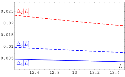
with Pν0 S(t)superscriptsubscript𝑃subscript𝜈0 S𝑡P_{\nu_{0}}^{\text{\,\tiny S}}(t) defined via Eqs. (11) and (21). We analyze the accuracy of the truncated FAPT expressions (22a) and compare them with the total sum (22b) using relative errors ΔN[L]=1ΓHbb¯(1)[L;N]/ΓHbb¯(1);[L]subscriptΔ𝑁delimited-[]𝐿1superscriptsubscriptΓ𝐻𝑏¯𝑏1𝐿𝑁superscriptsubscriptΓ𝐻𝑏¯𝑏1delimited-[]𝐿\Delta_{N}[L]=1-\Gamma_{H\to b\overline{b}}^{\,(1)}[L;N]/\Gamma_{H\to b\overline{b}}^{(1);\infty}[L]. In Fig. 1 we show these errors for N=2𝑁2N=2, N=3𝑁3N=3, and N=4𝑁4N=4 in the analyzed range of L[11,13.7]𝐿1113.7L\in[11,13.7]. We see that already ΓHbb¯(1)[L;2]superscriptsubscriptΓ𝐻𝑏¯𝑏1𝐿2\Gamma_{H\to b\overline{b}}^{\,(1)}[L;2] gives an accuracy of the order of 2.5%, whereas ΓHbb¯(1)[L;3]superscriptsubscriptΓ𝐻𝑏¯𝑏1𝐿3\Gamma_{H\to b\overline{b}}^{\,(1)}[L;3] is of the order of 1%.

Refer to caption   Refer to caption

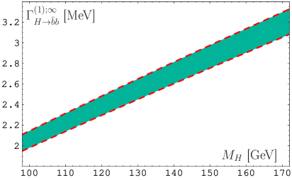
Figure 1: Left panel: The relative errors ΔN[L]subscriptΔ𝑁delimited-[]𝐿\Delta_{N}[L], N=2,3𝑁23N=2,3 and 444, of the truncated FAPT in comparison with the exact summation result, Eq. (22b). Right panel: The width ΓHbb¯subscriptΓ𝐻𝑏¯𝑏\Gamma_{H\to b\overline{b}} as a function of the Higgs boson mass MHsubscript𝑀𝐻M_{H} in the resummed FAPT. The width of the shaded strip is due to the overall uncertainties, induced by the uncertainties of the resummation procedure and the pole mass error-bars. Both panels show the results obtained in the one-loop FAPT [24].

Looking in the left panel of Fig. 1, we understand that in order to have an accuracy better than 0.5%, we need to take into account the 4-th correction. We also verified that the uncertainty due to P(t)𝑃𝑡P(t)-modelling is small, 0.6%less-than-or-similar-toabsentpercent0.6\lesssim 0.6\%, while the m¯b(m¯b2)subscript¯𝑚𝑏superscriptsubscript¯𝑚𝑏2\overline{m}_{b}(\overline{m}_{b}^{2})-induced uncertainty is of the order of 2%percent22\%. The overall uncertainty then is of the order of 3%percent33\%, see in the right panel of Fig. 1.

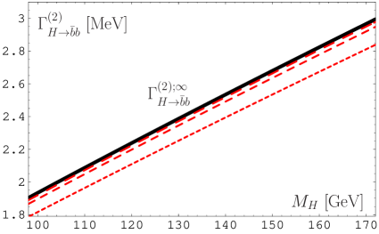
Qualitatively, the same picture is reproduced at the two-loop order [24]. In the left panel of Fig. 2, we discuss the convergence properties of the decay widths, truncated at the order N𝑁N, relative to the resummed two-loop result ΓHbb¯(2);(MH)superscriptsubscriptΓ𝐻𝑏¯𝑏2subscript𝑀𝐻\Gamma_{H\to b\overline{b}}^{(2);\infty}(M_{H}). We see that our conclusions drawn from the one-loop analysis remain valid. Indeed, ΓHbb¯(2)(MH;2)superscriptsubscriptΓ𝐻𝑏¯𝑏2subscript𝑀𝐻2\Gamma_{H\to b\overline{b}}^{(2)}(M_{H};2) deviates from the resummed quantity by not more than 2%, whereas ΓHbb¯(2)(MH;3)superscriptsubscriptΓ𝐻𝑏¯𝑏2subscript𝑀𝐻3\Gamma_{H\to b\overline{b}}^{(2)}(M_{H};3) reaches an even higher precision level of the order of 0.7%.

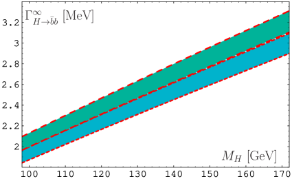
In the right panel of Fig. 2, we show the results for the decay width ΓHbb¯(MH)superscriptsubscriptΓ𝐻𝑏¯𝑏subscript𝑀𝐻\Gamma_{H\to b\overline{b}}^{\infty}(M_{H}) in the resummed two-loop FAPT, varying the mass in the interval m^(2)=8.22±0.13subscript^𝑚2plus-or-minus8.220.13\hat{m}_{(2)}=8.22\pm 0.13 GeV according to the Penin–Steinhauser estimate m¯b(m¯b2)=4.35±0.07subscript¯𝑚𝑏superscriptsubscript¯𝑚𝑏2plus-or-minus4.350.07\overline{m}_{b}(\overline{m}_{b}^{2})=4.35\pm 0.07 GeV [28]. Comparing this outcome with the one-loop result—upper strip in the same panel of this figure—reveals a 5% reduction of the two-loop estimate. This reduction consists of two parts: one part (+7%absentpercent7\approx+7\%) is due to the difference m^(1)2m^(2)2superscriptsubscript^𝑚12superscriptsubscript^𝑚22\hat{m}_{(1)}^{2}-\hat{m}_{(2)}^{2} in both approximations, while the other (2%absentpercent2\approx-2\%) comes from the difference in the values of RS(MH)subscript𝑅𝑆subscript𝑀𝐻R_{S}(M_{H}) in the one- and the two-loop approximations.
Refer to caption Refer to caption

Figure 2: Left panel: The two-loop width ΓHbb¯subscriptΓ𝐻𝑏¯𝑏\Gamma_{H\to b\overline{b}} as a function of the Higgs-boson mass MHsubscript𝑀𝐻M_{H} in the resummed (black solid line) and the truncated (at the order N𝑁N) FAPT [24]. Here, the short-dashed line corresponds to N=1𝑁1N=1, the dashed one to N=2𝑁2N=2, and the long-dashed line to N=3𝑁3N=3. Right panel: The two-loop width ΓHbb¯superscriptsubscriptΓ𝐻𝑏¯𝑏\Gamma_{H\to b\overline{b}}^{\infty} as a function of the Higgs-boson mass MHsubscript𝑀𝐻M_{H} in the resummed FAPT is shown (lower strip). The upper strip shows the corresponding one-loop result.

4 Application to the vector correlator Adler function

Now we analyze the Adler function of the vector correlator. We model the generating function of the perturbative coefficients dnsubscript𝑑𝑛d_{n} [31] (note that here d1=1subscript𝑑11d_{1}=1, so that d~n=dnsubscript~𝑑𝑛subscript𝑑𝑛\tilde{d}_{n}=d_{n})

DV[L]=d0+n=1dn(αs[L]π)nsubscript𝐷Vdelimited-[]𝐿subscript𝑑0superscriptsubscript𝑛1subscript𝑑𝑛superscriptsubscript𝛼𝑠delimited-[]𝐿𝜋𝑛\displaystyle D_{\text{V}}[L]=d_{0}+\sum_{n=1}^{\infty}d_{n}\,\left(\frac{\alpha_{s}[L]}{\pi}\right)^{n} (23)

using a generalized Lipatov-like model:

dnVsuperscriptsubscript𝑑𝑛V\displaystyle d_{n}^{\text{V}} =\displaystyle= cn1δn+1nδ21Γ(n),superscript𝑐𝑛1superscript𝛿𝑛1𝑛superscript𝛿21Γ𝑛\displaystyle c^{n-1}\,\frac{\delta^{n+1}-n}{\delta^{2}-1}\,\Gamma(n)\,, (24a)
PV(t)subscript𝑃V𝑡\displaystyle P_{\text{V}}(t) =\displaystyle= δet/cδ(t/c)et/cc(δ21).𝛿superscript𝑒𝑡𝑐𝛿𝑡𝑐superscript𝑒𝑡𝑐𝑐superscript𝛿21\displaystyle\frac{\delta\,e^{-t/c\delta}-(t/c)\,e^{-t/c}}{c\left(\delta^{2}-1\right)}\,. (24b)

Our predictions, obtained with this generating function by fitting the two known coefficients d~2subscript~𝑑2\tilde{d}_{2} and d~3subscript~𝑑3\tilde{d}_{3}, have been included in Table 1 (see [24]). We observe a good agreement between our estimate d4V=27.1superscriptsubscript𝑑4V27.1d_{4}^{\text{V}}=27.1 and the value 27.4, calculated recently by Chetyrkin et al. in Ref. [31]. Would we use instead a fitting procedure, which would take into account the fourth-order coefficient d4subscript𝑑4d_{4} in order to predict d5subscript𝑑5d_{5}, we should readjust the model parameters in (24) to the new values {c=3.5526,δ=1.32453}formulae-sequence𝑐3.5526𝛿1.32453\left\{c=3.5526,~{}\delta=1.32453\right\}. In order to explore to what extent the exact knowledge of the higher-order coefficients dnsubscript𝑑𝑛d_{n} is important, we employed our model (24) in [24] with different values of the parameters: c=3.63𝑐3.63c=3.63 and δ=1.3231𝛿1.3231\delta=1.3231. These values were selected in order to reproduce the exact value of the coefficient d4=27.4subscript𝑑427.4d_{4}=27.4 by the value, close to the Naive Non-Abelization (NNA) prediction [32]. The difference between the resummed results of the two models in the region of Nf=4subscript𝑁𝑓4N_{f}=4 appears to be very small — of the order of 0.2%percent0.20.2\%.

Table 1: Coefficients dnsubscript𝑑𝑛d_{n} for the Adler-function series with Nf=4subscript𝑁𝑓4N_{f}=4. The numbers in the square brackets denote the lower and the upper limits of the Improved NNA (INNA) estimates.

PT coefficients  d1subscript𝑑1d_{1}\vphantom{{}^{|}_{|}}  d2subscript𝑑2d_{2}  d3subscript𝑑3d_{3}  d4subscript𝑑4d_{4}  d5subscript𝑑5d_{5} pQCD results with Nf=4subscript𝑁𝑓4N_{f}=4 [31] 111\vphantom{{}^{|}_{|}}  1.52  2.59  27.4  — Model (24) with c=3.555,δ=1.3245formulae-sequence𝑐3.555𝛿1.3245c=3.555,~{}\delta=1.3245 111\vphantom{{}^{|}_{|}}  1.52  2.59  27.1  2024 Model (24) with c=3.553,δ=1.3245formulae-sequence𝑐3.553𝛿1.3245c=3.553,~{}\delta=1.3245 111\vphantom{{}^{|}_{|}}  1.52  2.60  27.3  2025 Model (24) with c=3.630,δ=1.3231formulae-sequence𝑐3.630𝛿1.3231c=3.630,~{}\delta=1.3231 111\vphantom{{}^{|}_{|}}  1.53  2.26  20.7  2020 “INNA” prediction of  [24] 111\vphantom{{}^{|}_{|}}  1.44  [3.5,9.6]3.59.6[3.5,9.6]  [20.4,48.1]20.448.1[20.4,48.1]  [674,2786]6742786[674,2786]

We also show in Table 1 the dnsubscript𝑑𝑛d_{n} estimates obtained by using the Improved NNA (INNA) approximation, developed in our last paper [24] by taking into account not only the b0nαsnsuperscriptsubscript𝑏0𝑛superscriptsubscript𝛼𝑠𝑛b_{0}^{n}\alpha_{s}^{n} terms, but also the b1kb0n2kαsnsuperscriptsubscript𝑏1𝑘superscriptsubscript𝑏0𝑛2𝑘superscriptsubscript𝛼𝑠𝑛b_{1}^{k}b_{0}^{n-2k}\alpha_{s}^{n} ones. This technique produces predictions for higher-order coefficients in terms of intervals for the dnsubscript𝑑𝑛d_{n}values. We see that our model predictions for the d5subscript𝑑5d_{5} coefficient are all inside the INNA interval.

Then, we have

DVAPT(Q2)superscriptsubscript𝐷VAPTsuperscript𝑄2\displaystyle D_{\text{V}}^{\text{APT}}(Q^{2}) =\displaystyle= 1+n1dnVπn𝒜nglob(Q2),1subscript𝑛1subscriptsuperscript𝑑V𝑛superscript𝜋𝑛superscriptsubscript𝒜𝑛globsuperscript𝑄2\displaystyle 1+\sum_{n\geq 1}\frac{d^{\text{V}}_{n}}{\pi^{n}}\,\mathcal{A}_{n}^{\text{\tiny glob}}(Q^{2})\,, (25a)
DVAPT(Q2;N)superscriptsubscript𝐷VAPTsuperscript𝑄2𝑁\displaystyle D_{\text{V}}^{\text{APT}}(Q^{2};N) =\displaystyle= 1+n=1NdnVπn𝒜nglob(Q2).1superscriptsubscript𝑛1𝑁subscriptsuperscript𝑑V𝑛superscript𝜋𝑛superscriptsubscript𝒜𝑛globsuperscript𝑄2\displaystyle 1+\sum_{n=1}^{N}\frac{d^{\text{V}}_{n}}{\pi^{n}}\,\mathcal{A}_{n}^{\text{\tiny glob}}(Q^{2})\,. (25b)

Refer to caption

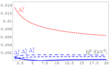
Figure 3: The relative errors ΔNV(Q2)subscriptsuperscriptΔV𝑁superscript𝑄2\Delta^{\text{V}}_{N}(Q^{2}) evaluated for different values of N𝑁N: N=1𝑁1N=1 (short-dashed red line), N=2𝑁2N=2 (solid blue line), N=3𝑁3N=3 (dashed blue line), and N=4𝑁4N=4 (long-dashed blue line) of the truncated APT given by Eq. (25b), in comparison with the exact result of the APT resummation procedure.

The global-APT resummation result for DVAPT(Q2)superscriptsubscript𝐷VAPTsuperscript𝑄2D_{\text{V}}^{\text{APT}}(Q^{2}) can be estimated using our resummation formulas from [18, 23, 24], which we shortly explained in Sect. 2. We show in Fig. 3 the relative errors ΔNV(Q2)=1DVAPT(Q2;N)/DVAPT(Q2)superscriptsubscriptΔ𝑁Vsuperscript𝑄21superscriptsubscript𝐷VAPTsuperscript𝑄2𝑁superscriptsubscript𝐷VAPTsuperscript𝑄2\Delta_{N}^{\text{V}}(Q^{2})=1-D_{\text{V}}^{\text{APT}}(Q^{2};N)/D_{\text{V}}^{\text{APT}}(Q^{2}) evaluated in the range Q2[2,20]superscript𝑄2220Q^{2}\in[2,20] GeV2 for four values N=1,2,3,4𝑁1234N=1,2,3,4. We observe from this figure that already DVAPT(Q2;1)superscriptsubscript𝐷VAPTsuperscript𝑄21D_{\text{V}}^{\text{APT}}(Q^{2};1) provides an accuracy in the vicinity of 1%, whereas DVAPT(Q2;2)superscriptsubscript𝐷VAPTsuperscript𝑄22D_{\text{V}}^{\text{\tiny APT}}(Q^{2};2) is smaller then 0.1% in the interval Q2=120superscript𝑄2120Q^{2}=1-20 GeV2. This means that there is no real need to calculate further corrections: at the level of an accuracy of the order of 1% it is quite enough to take into account only the terms up to d2subscript𝑑2d_{2}. Again, we verified that this conclusion is stable with respect to the variation of the model PV(t)subscript𝑃V𝑡P_{\text{V}}(t) parameters. This conclusion is in some sense surprising: The best order of truncation of the FAPT series in the region Q2=220superscript𝑄2220Q^{2}=2-20 GeV2 is reached by the N2LO approximation, i.e., by keeping just the d2subscript𝑑2d_{2}-term.

5 Conclusions

We described here the resummation approach in the global versions of both APT and FAPT for the one- and two-loop running of the effective QCD coupling. We argued that this approach produces finite answers, provided the generating function P(t)𝑃𝑡P(t) of the perturbative coefficients dnsubscript𝑑𝑛d_{n} is known. We considered two applications of our approach to the physical problems of current interest.

In the case of the Higgs boson decay, Hb¯b𝐻¯𝑏𝑏H\to\bar{b}b, the main conclusion is that to achieve a truncation accuracy of the order of 1% for the width ΓHbb¯(MH)subscriptΓ𝐻𝑏¯𝑏subscript𝑀𝐻\Gamma_{H\to b\overline{b}}(M_{H}) it is enough to take into account up to the third correction — in complete agreement with Kataev&Kim [33]. In the case of the vector-current Adler function, 𝒟V(Q2)subscript𝒟Vsuperscript𝑄2\mathcal{D}_{\text{V}}(Q^{2}), the truncation accuracy is of the order 0.1%, already reached at N2LO, i. e., by taking into account up to the second-order correction.

In our approach the knowledge of higher-order coefficients, d4subscript𝑑4d_{4}, is needed in order to construct a reliable model for the generating functions P(t)𝑃𝑡P(t). Meanwhile, we showed that the exact values of still higher coefficients, d5subscript𝑑5d_{5}, are not so important.

Acknowledgements

I wish to thank Sergey Mikhailov and Nico Stefanis for a fruitful collaboration, and Konstantin Chetyrkin, Andrey Grozin, Andrey Kataev and Alexey Pivovarov for useful remarks and discussions. This work was supported in part by the Russian Foundation for Fundamental Research, grant No.   08-01-00686, the BRFBR–JINR Cooperation Programme, contract No. F10D-001, and the Heisenberg–Landau Programme under Grant 2010.

References

  • [1] N. N. Bogolyubov, A. A. Logunov, and D. V. Shirkov, Soviet Physics JETP 10 (1960) 574.
  • [2] A. V. Radyushkin, JINR Rapid Commun. 78 (1996) 96; [JINR Preprint, E2-82-159, 26 Febr. 1982; arXiv: hep-ph/9907228].
  • [3] N. V. Krasnikov and A. A. Pivovarov, Phys. Lett. B116 (1982) 168.
  • [4] Y. L. Dokshitzer, G. Marchesini, and B. R. Webber, Nucl. Phys. B469, 93 (1996).
  • [5] H. F. Jones and I. L. Solovtsov, Phys. Lett. B349, 519 (1995).
  • [6] H. F. Jones, I. L. Solovtsov, and O. P. Solovtsova, Phys. Lett. B357, 441 (1995).
  • [7] M. Beneke and V. M. Braun, Phys. Lett. B348 (1995) 513.
  • [8] P. Ball, M. Beneke, and V. M. Braun, Nucl. Phys. B452 (1995) 563.
  • [9] D. V. Shirkov and I. L. Solovtsov, JINR Rapid Commun. 2 [76] (1996) 5; Phys. Rev. Lett. 79 (1997) 1209; Theor. Math. Phys. 150 (2007) 132.
  • [10] Y. A. Simonov, Phys. Atom. Nucl. 65 (2002) 135.
  • [11] D. V. Shirkov, Theor. Math. Phys. 127, 409 (2001); Eur. Phys. J. C22, 331 (2001).
  • [12] A. I. Karanikas and N. G. Stefanis, Phys. Lett. B504 (2001) 225; B636, 330 (2006).
  • [13] N. G. Stefanis, W. Schroers, and H.-C. Kim, Phys. Lett. B449 (1999) 299; Eur. Phys. J. C18 (2000) 137.
  • [14] N. G. Stefanis, Lect. Notes Phys. 616 (2003) 153.
  • [15] A. P. Bakulev, K. Passek-Kumerički, W. Schroers, and N. G. Stefanis, Phys. Rev. D70 (2004) 033014.
  • [16] A. P. Bakulev, S. V. Mikhailov, and N. G. Stefanis, Phys. Rev. D72 (2005) 074014, 119908(E); ibid. 75 (2007) 056005; 77 (2008) 079901(E).
  • [17] A. P. Bakulev, A. I. Karanikas, and N. G. Stefanis, Phys. Rev. D72 (2005) 074015.
  • [18] A. P. Bakulev Phys. Elem. Part. Nucl. 40 (2009) 715.
  • [19] N. G. Stefanis, arXiv:0902.4805 [hep-ph].
  • [20] S. V. Mikhailov, JHEP 06 (2007) 009 [hep-ph/0411397].
  • [21] M. Neubert, Phys. Rev. D51 (1995) 5924.
  • [22] G. Cvetic and C. Valenzuela, Phys. Rev. D74 (2006) 114030 [hep-ph/0608256].
  • [23] A. P. Bakulev and S. V. Mikhailov, in Proc. Int. Seminar on Contemp. Probl. of Part. Phys., dedicated to the memory of I. L. Solovtsov, Dubna, Jan. 17–18, 2008., Eds. A. P. Bakulev et al. (JINR, Dubna, 2008), pp. 119–133 (arXiv:0803.3013).
  • [24] A. P. Bakulev, S. V. Mikhailov, and N. G. Stefanis, JHEP 1006 (2010) 085.
  • [25] P. A. Baikov, K. G. Chetyrkin, and J. H. Kühn, Phys. Rev. Lett. 96 (2006) 012003.
  • [26] K. G. Chetyrkin and M. Steinhauser, Phys. Rev. Lett. 83, 4001 (1999).
  • [27] K. G. Chetyrkin and M. Steinhauser, Nucl. Phys. B573 (2000) 617.
  • [28] A. A. Penin and M. Steinhauser, Phys. Lett. B538 (2002) 335.
  • [29] A. L. Kataev and V. V. Starshenko, Mod. Phys. Lett. A10 (1995) 235.
  • [30] K. G. Chetyrkin, B. A. Kniehl, and A. Sirlin, Phys. Lett. B402 (1997) 359.
  • [31] P. A. Baikov, K. G. Chetyrkin, and J. H. Kühn, Phys. Rev. Lett. 101 (2008) 012002; ibid. 104 (2010) 132004.
  • [32] D. J. Broadhurst and A. L. Kataev, Phys. Lett. B315 (1993) 179; ibid. B544 (2002) 154.
  • [33] A. L. Kataev and V. T. Kim, in Proc. Int. Seminar on Contemp. Probl. of Part. Phys., dedicated to the memory of I. L. Solovtsov, Dubna, Jan. 17–18, 2008., Eds. A. P. Bakulev et al. (JINR, Dubna, 2008), pp. 167–182 (arXiv:0804.3992);
    PoS ACAT08 (2009) 004.