The Sparsest Clusters With O Stars
Abstract
There is much debate on how high-mass star formation varies with environment, and whether the sparsest star-forming environments are capable of forming massive stars. To address this issue, we have observed eight apparently isolated OB stars in the SMC using HST’s Advanced Camera for Surveys. Five of these objects appear as isolated stars, two of which are confirmed to be runaways. The remaining three objects are found to exist in sparse clusters, with companion stars revealed, having masses of 1 – 4 . Stochastic effects dominate in these sparse clusters, so we perform Monte Carlo simulations to explore how our observations fit within the framework of empirical, galactic cluster properties. We generate clusters using a simplistic –2 power-law distribution for either the number of stars per cluster () or cluster mass (). These clusters are then populated with stars randomly chosen from a Kroupa IMF. We find that simulations with cluster lower-mass limits of and match best with observations of SMC and Galactic OB star populations. We examine the mass ratio of the second-most massive and most massive stars , finding that our observations all exist below the 20th percentile of our simulated clusters. However, all of our observed clusters lie within the parameter space spanned by the simulated clusters, although some are in the lowest 5th percentile frequency. These results suggest that clusters are built stochastically by randomly sampling stars from a universal IMF with a fixed stellar upper-mass limit. In particular, we see no evidence to suggest a relation. Our results may be more consistent with core accretion models of star formation than with competitive accretion models, and they are inconsistent with the proposed steepening of the integrated galaxy IMF (IGIMF).
Subject headings:
galaxies: Magellanic Clouds – galaxies: star clusters – galaxies: stellar content – stars: early-type – stars: formation1. Introduction
Most observational properties of galaxies and stellar populations are directly influenced by star formation. Massive stars, although small in number, disproportionally affect observables such as the integrated light from galaxies, feedback effects, star formation rates, and many others. However, there is significant debate regarding the conditions under which massive stars form. The competitive accretion model of star formation requires that a population of low-mass stars must form in the presence of a high-mass star (e.g. Bonnell et al. 2004), while the core accretion model of star formation allows for massive stars to form in relative isolation (e.g. Krumholz et al. 2009). Empirical studies are similarly divided on the connection between cluster mass and massive star formation. A physical relationship between the two (e.g. Weidner & Kroupa 2006, hereafter WK06) would indicate that massive stars always form in clusters, while random statistical sampling (e.g. Elmegreen 2000) would indicate that massive stars preferentially form in clusters. One observational method to differentiate between these theories is to examine the sparsest environments where massive stars are found. A targeted study of field massive stars can quantify limitations on the minimum stellar groupings needed for massive star formation. Such a study, which we present in this work, provides direct observational constraints for the two competing theories of star formation.
The core accretion model suggests that stars of all masses form by a fragmentation process in molecular clouds, where cores collapsing due to self-gravity represent the mass available to form an individual star or stellar multiple system (e.g. Shu et al. 1987). In this model, massive stars must necessarily form from massive cores; however, it is unclear how such massive cores (up to hundreds of Jeans masses) can collapse without further fragmentation. Analytic models by Krumholz & McKee (2008) suggest that sufficiently dense clouds having surface densities g/cm-2 will trap stellar and accretion radiation that heats clouds and prevents further fragmentation. Additionally, 3-D hydrodynamic simulations by Krumholz et al. (2009) reveal that self-shielding occurs along filaments resulting from gravitational and Rayleigh-Taylor instabilities, thereby channeling gas onto massive stars despite radiation pressures that dominate gravitational forces. These simulations result in the formation of a high-mass star or multiple system with a small companion population of low-mass stars. Similarly, Spaans & Silk (2000) show that the star formation properties of a gravitationally collapsing molecular cloud are highly dependent upon the equation of state of that cloud. For a cloud polytropic equation of state given by where is the thermal pressure and is the gas density, they concluded that yields a peaked stellar initial mass function (IMF) rather than a power-law distribution. Li et al. (2003) conduct further simulations and find that molecular clouds with will most likely result in the formation of massive, isolated stars.
In contrast, the competitive accretion model suggests that fragmentation only produces low-mass stars, with high-mass stars formed by winning a competition for the remaining gas (e.g. Zinnecker 1982). In this scenario, the mass of a star is highly dependent upon the star-forming environment, with high-mass stars preferentially located at the bottom of the gravitational potential where the majority of a cluster gas reservoir gets funneled (Bonnell et al. 2001). This model of massive star formation requires that massive stars form in a clustered environment, with an explicit relation between the mass of a cluster () and the mass of the most massive star in the cluster () given by (Bonnell et al. 2004). Thus, competitive accretion forms massive stars along with a fully populated cluster of lower mass companion stars (Bonnell et al. 2007).
One of the primary differences between the observational predictions of these models is in the formation of high-mass stars in low environments. Competitive accretion argues that formation of a high-mass star in a low-mass cluster is extremely difficult, while core accretion places no formal constraint on cluster mass. The competitive accretion model implies that the IMF is not a universal property of star formation, but instead tends to limit for a given . However, the IMF has been robustly verified for a wide range of star-forming environments, leading many to argue that , the upper stellar mass limit, is a universal property of star formation, regardless of environment (see Elmegreen 2000, 2006, 2008). In the case of a universal IMF, the relationship between and is determined by the statistical mean (Oey & Clarke 2005). Not everyone agrees with the universality of the IMF; for example, WK06 argue for the existence of a deterministic - relation using analytic models. They further their argument by aggregating a data sample of Galactic clusters from which they find a strong correlation between and , closely following the derived - relation in Weidner & Kroupa (2004). Weidner et al. (2010a), who update and greatly expand the observational data set, conclude using a variety of statistical tests, that it is highly unlikely that the sample of Galactic clusters is generated from random sampling of a universal IMF.
However, Selman & Melnick (2008), using the same data from WK06, argue that the correlation of with may be caused by the quick dispersal of clusters dominated by a single massive star due to gravitational instabilities. Since these objects would no longer be identifiable as clusters, such a dispersal effect would bias the WK06 cluster sample against clusters that formed with a flatter-than-Salpeter mass function, leaving behind only those clusters that follow a more standard Salpeter mass function. Maschberger & Clarke (2008) complement the WK06 data set with a sample of very small clusters from Testi et al. (1997) and find that the resultant ensemble of clusters does not significantly deviate from the expectations of a universal stellar IMF, when examining the correlation between the number of stars in a cluster () and . They argue that analyses using instead of are more reliable since is a directly observable quantity, while must be inferred. They caution that observational and sample selection effects can greatly influence the correlation of with or and that much more observational data is needed to reach a conclusion.
A - relation, if it exists, has broad implications for cumulative stellar populations of galaxies. The power-law form of the cluster mass function is robust, similar to the IMF, with empirical derivations from a wide range of Galactic objects and environments, generally consistent with a power-law slope of –1.7 to –2.3 (§3.2). Coupling the cluster mass function, which is highly weighted towards low-mass clusters, with a deterministic - relation can have a large effect on the integrated galactic initial mass function (IGIMF) for stars. The primary consequences include a decrease in the expected number of OB stars within galaxies and an overall steepening of the IGIMF for the composite stellar population of a galaxy (Kroupa & Weidner 2003; Weidner & Kroupa 2005). A steepened IGIMF appears to successfully reproduce a variety of poorly-understood observationally-derived relations, including the dwarf galaxy mass-metallicity relation (Köppen et al. 2007), global correlations between H to UV flux ratios and galaxy mass (Hoversten & Glazebrook 2008; Lee et al. 2009; Meurer et al. 2009), and sharp radial surface brightness truncations in H compared to more extended-UV emission in the outer disks of nearby galaxies (Thilker et al. 2007; Pflamm-Altenburg et al. 2009). Such observational relations appear to arise naturally from clustered star formation and the - relation implicit to a steepened IGIMF. Maschberger et al. (2010) found evidence of a steepened IGIMF in the competitive accretion simulations of Bonnell et al. (2003, 2008), linking these two theories under their common assumption of a - relation. Considering the far-reaching implications of a steepened IGIMF, it is of utmost importance to examine its validity using observational constraints of isolated O stars.
One observational method to test the assertion of a - relation is to look for isolated, massive star formation. Field O stars are abundant in the literature (e.g., Massey et al. 1995) and may account for 25-30% of the O star population in a galaxy (Oey, et al. 2004). While many of these stars are likely to be runaway stars from clusters, the remainder of field stars with no evidence of companions would be difficult to incorporate into the - relation proposed by WK06 and inherent to the theory of competitive accretion. In a study of Galactic field O stars, de Wit et al. (2004, 2005) find that % of all Galactic O stars appear to have formed in isolation, without the presence of a nearby cluster or evidence of a large space velocity indicative of a runaway star. This value is in agreement with the 5% of isolated O stars (defined as O stars without any companion O or B stars) found from Monte Carlo simulations of clusters (Parker & Goodwin 2007).
In this paper, we examine the stellar environment around field O stars to probe the limiting cases where O stars form in the sparsest stellar groups, or in near isolation.
2. Observations
2.1. HST Imaging Observations
We target field O stars in the SMC for this study because this nearby galaxy offers a view unobscured by gas and dust, allowing clear identification of the field massive stars and any low-mass companions. Our targets are taken from the work of Oey et al. (2004), who applied a friends-of-friends algorithm to photometrically identify OB star candidates, thereby identifying clusters and field stars in this sample. For this study, all of the targets were spectroscopically verified as O or early B stars, and all appeared isolated in ground-based imaging. In a pilot SNAP program, we exploit the 0.05/px spatial resolution of the Advanced Camera for Surveys (ACS) Wide-Field Camera aboard the Hubble Space Telescope (HST) to search for low-mass stars associated with the target OB stars. Unfortunately, Cycle 14 had an unusually low SNAP return, and we obtained observations of only eight targets. Table 1 lists our sample. Column 1 gives the star’s ID from the catalog of Azzopardi & Vigneau (1975); the star smc-16 was catalogued by Massey et al. (1995). Columns 2, 3, and 4 list the right ascension, declination, and V magnitude, respectively, taken from Massey (2002). Column 5 gives the spectral types, in some cases derived from our observations described below in §2.3. Column 6 gives our mass estimate derived from the spectral type as described below, in §2.4. Column 7 gives our measured heliocentric radial velocities (see §2.3).
| Field OB Star | RAaaFrom Massey (2002). | DecaaFrom Massey (2002). | VaaFrom Massey (2002). | Spectral TypebbObserved with the IMACS multislit spectrograph on the 6.5m Magellan/Baade telescope, unless otherwise stated. | Mass () | RVbbObserved with the IMACS multislit spectrograph on the 6.5m Magellan/Baade telescope, unless otherwise stated. (km s-1) |
|---|---|---|---|---|---|---|
| smc16 | 01:00:43.94 | -72:26:04.9 | 14.38 | O9 V | ||
| AzV 58 | 00:49:57.84 | -72:51:54.4 | 14.29 | B0.5 III | ||
| AzV 67 | 00:50:11.13 | -72:32:34.8 | 13.64 | O8 V | ||
| AzV 106 | 00:51:43.36 | -72:37:24.9 | 14.18 | B1 II | ||
| AzV 186 | 00:57:26.99 | -72:33:13.3 | 13.98 | O8 III((f))ccFrom Massey (2009). | ||
| AzV 223 | 00:59:13.41 | -72:39:02.2 | 13.66 | O9 IIddFrom Evans (2006). | eeObserved with the MIKE echelle spectrograph on the 6.5m Magellan/Clay telescope. | |
| AzV 226 | 00:59:20.69 | -72:17:10.3 | 14.24 | O7 III((f))ccFrom Massey (2009). | ||
| AzV 302 | 01:02:19.01 | -72:22:04.4 | 14.20 | O8.5 VeeObserved with the MIKE echelle spectrograph on the 6.5m Magellan/Clay telescope. | eeObserved with the MIKE echelle spectrograph on the 6.5m Magellan/Clay telescope. |
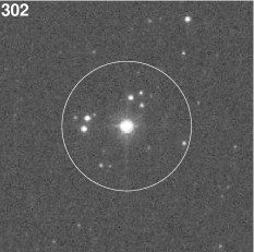
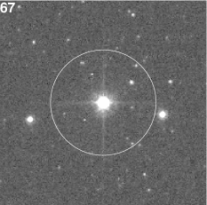
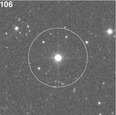
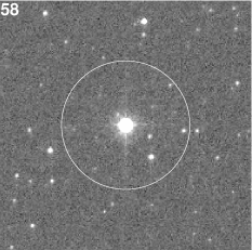
We obtained exposures of 6 seconds in the F555W band and 18 seconds in the F814W band. Figure 1 shows the F814W images of each object, with a circle of radius one parsec (3.4 arcsec) for reference, adopting an SMC distance of 60 kpc (Harries et al. 2003). The F555W exposures are complete down to 21st magnitude while the F814W are complete down to 22nd magnitude.
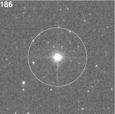
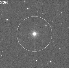
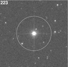
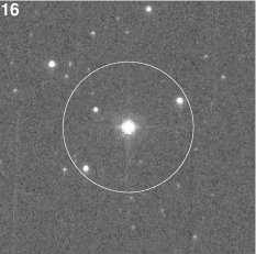
For each HST field, we use the IRAF DAOPHOT package to identify stars and obtain their photometry, using a combination of aperture photometry and PSF fitting. The aperture photometry is more reliable due to an undersampled PSF; however, PSF fitting was unavoidable in the case of close companions. The aperture photometry was done with an aperture radius of six pixels, while PSF fitting was done with a two-pixel FWHM and corrected to match the six-pixel aperture. For the F555W images, 3–5% of stars require PSF fitting, while in the F814W band, 10–15% require PSF fitting. PSF fitting did not reveal close companions for any of the target stars; however, the PSF subtraction of the target stars was very non-uniform, so companions cannot be entirely ruled out.
We used two separate methods to identify possible companion stars associated with the targets: (1) an analysis of the stellar density surrounding the OB star and (2) a friends-of-friends algorithm. For the first method, we computed the stellar surface density of the field as a function of radius from the target OB star. We performed this analysis using the F814W exposures, since they probe to a fainter magnitude than the F555W images. To measure the average stellar density of the field, we used an annulus centered on the OB star, with an inner radius ranging from 5 to 10, and an outer radius 10 beyond the inner radius; the annuli were positioned to avoid any obvious stellar clustering. We define a density enhancement to occur when the observed stellar density is higher than the average stellar density of the field, including the statistical uncertainty. The probability that the observed stellar distribution matches the expected Poisson distribution, for a given background stellar density, is:
| (1) |
where is the expected star count within a given radius and is the observed star count within that radius. A more useful value, which we designate the “field probability” , is the likelihood that the population follows the stellar density of the field:
| (2) |
The right term in equation 2 yields the probability of observing more than stars within a certain radius, and so represents the probability of obtaining the background field. A smaller therefore indicates an increased likelihood of clustering.
To examine the stellar environment near each target star, we plot the cumulative stellar density as a function of radius from the target OB star in Figure 2. The horizontal lines show the measured background density of each field. We were unable to detect stars within the wings of the target star, which typically extended to a radius of 0.2 pc. Thus, the actual cumulative stellar densities may be higher than those observed. Table 2 lists the angular and physical radius at which is minimized in columns 2 and 3, respectively. The value of is listed in column 4 for targets showing a density enhancement.


| Field | Angular Size (″) | (pc) | (pc) | Field IMF | |
|---|---|---|---|---|---|
| smc16 | … | … | … | 0.52 | |
| AzV 58 | … | … | … | 0.43 | |
| AzV 67 | 10.3 | 1.5 | 0.114 | 0.50 | |
| AzV 106 | 6.9 | 1.0 | 0.047 | 0.43 | |
| AzV 186 | … | … | … | 0.46 | |
| AzV 223 | … | … | … | 0.47 | |
| AzV 226 | … | … | … | 0.48 | |
| AzV 302 | 4.8 | 0.7 | 0.0001 | 0.58 |
We also searched for density enhancements with a friends-of-friends algorithm applied to our F814W images. This method defines group members to be all the stars within a fixed clustering length of another member of the same group. Following Battinelli (1991), we adopted a value for that maximizes the number of groups having at least three stars. The distributions of clusters vs. for each field are approximated well by normal distributions, and so we used gaussian functions to estimate . Figure 3 shows a representative example. The average for these observations is parsecs. Table 2 lists the clustering length of each field in column 5.

2.2. Minimal O Star Groups
As seen from the data in Figure 2 and Table 2, there are three stars that show robust evidence of small, associated stellar groups: AzV 67, AzV 106, and AzV 302. The field probabilities, , for these targets range from 0.01% to 11.4%. The friends-of-friends algorithm confirms the existence of stars within the clustering length in each of these fields. To examine the sensitivity to , we also ran the friends-of-friends code with values of pc, where this variation is equal to the standard deviation of in the sample (see above). For the smaller values, this yielded companions only for AzV 302; while the larger value resulted in associated stars for all targets in our sample. Thus, we are confident that the fitted peak values for are appropriate, and they support the identification of groups found by identifying density enhancements. We will refer to these sparse groups as “minimal O star groups”. AzV 186 is the only field to appear clustered using the friends-of-friends algorithm, but not the density enhancement algorithm. We identify only those fields that appear clustered using both algorithms, as minimal O star groups.
2.3. Isolated Field Stars
The remaining four targets (AzV 58, AzV 223, AzV 226, smc16) show no evidence of associated stars using either of the methods above. These are candidates for massive stars that formed in complete isolation. However, a substantial fraction of field O stars likely did not originate in the field at all, but rather are runaway stars from clusters (e.g., Blaauw 1961; Gies 1987; Hoogerwerf et al. 2001). Thus, we examine the likelihood that our isolated OB stars are runaways.
We are performing a complete spectroscopic survey of SMC field OB stars that is now underway, using primarily the IMACS multi-slit spectrograph on the 6.5-m Magellan/Baade telescope at Las Campanas Observatory (Lamb et al, in preparation). These data yield the stellar radial velocities and spectral classifications, and we will ultimately estimate the runaway fraction for these massive field stars. In the course of this survey, we obtained spectra of the target field OB stars in our HST imaging sample. Table 1 gives our measured heliocentric radial velocities and spectral classifications. Several stars were previously classified, and we either confirmed or revised the spectral types, as shown.
We identify two of these stars, smc16 and AzV 223, as runaways, defined as stars having 30 km s-1 difference (de Wit et al. 2005) from the SMC systemic velocity of km s-1 (Staveley-Smith et al. 1997). We note that Stanimirović et al. (2004) found the SMC to have a velocity gradient; however, the positions of our targets do lie between the 150 km s-1 and 160 km s-1 contours as plotted in Figure 3 of Stanimirović et al. (2004). The two runaway stars will be removed from analysis in all subsequent sections, since they are no longer located in the region of their formation. This leaves us with two, isolated, apparently non-runaway OB stars, AzV 58 and AzV 226. Assuming an isotropic distribution of runaway velocities, we still expect to miss a number of transverse runaways. The missed fraction depends on the velocity distribution of runaway stars; however, we estimate that typical ejection velocities of 60 km s-1 or 120 km s-1 would cause us to miss two or one transverse runaway(s), respectively. Therefore, transverse runaways may account for both our remaining isolated stars.
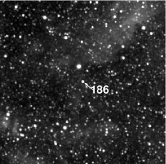
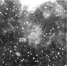
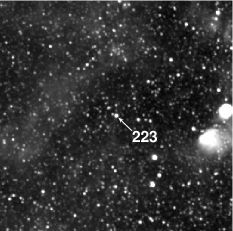
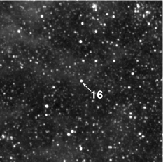
It is also informative to investigate the interstellar gas around these field OB stars (Figure 4). We examined the ionized gas around our target stars, using H data from the Magellanic Cloud Emission Line Survey (MCELS; Smith et al. 2000). Since gas is a necessary component of star formation, the presence of gas can help to constrain which stars may still be in the region of their formation. As a control group, all three of our minimal O star groups show H emission within 2.0 (35 pc), consistent with a physical association within these groups as sparse, young clusters. We also find that both confirmed runaway stars are far removed from any H emission. For the remaining isolated targets, the MCELS data show that AzV 58 and AzV 226 are located within Hii regions in the line of sight (Figure 4), while AzV 186 is far from any Hii regions. These results suggest that AzV 58 and AzV 226 may still be in the region of their formation and thus they remain candidates for isolated massive star formation.
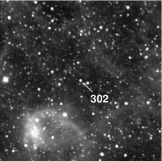
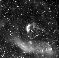
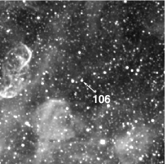
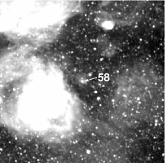
2.4. The IMF
We construct color-magnitude diagrams (CMD’s) from our ACS photometry, and use these to evaluate the IMF for the minimal O star groups as well as the field stars. We converted the photometric results from the F555W and F814W bands to Johnson V and Cousins I bands, respectively, following the synthetic transfer equations provided in Sirianni et al. (2005). These V and I band magnitudes were then extinction corrected using the SMC extinction maps provided by the Magellanic Cloud Photometric Survey (MCPS; Zaritsky, et al. 2002). MCPS provides two sets of stars for estimating extinction, the “hot” stars ( K K) and “cool” stars ( K K). We chose to average the extinction values of “cool” stars within 1 of the target star for the extinction calculation, as these objects better trace the sparse field population of our observations. The “hot” stars tend to trace active, clustered star formation with high gas content, yielding extinction values up to half a magnitude higher than those typically found in the “cool” stars.
We then calculated absolute magnitudes using a distance modulus of 18.9 (Harries et al. 2003). Comparisons of our photometry with MCPS photometry typically show differences less than 0.1 mag, with I-band matching more closely than . On average, our photometry appears fainter than that of the MCPS in both V and I bands. For stars fainter than 16th magnitude, Zaritsky et al. (2002) find that stellar crowding may play a factor in spuriously brightening the MCPS photometry when compared with the OGLE catalog (Udalski et al. 1998), which they deem to be superior in this regime. Since nearly all stars in our fields are fainter than 16th magnitude, the difference between our photometry and MCPS photometry is likely due to these crowding effects.
We used Geneva stellar evolutionary tracks to extract mass estimates from our photometry. These tracks are based on the ATLAS9 no-overshoot models at SMC metallicity, calculated by Charbonnel et al. (1993) and have been converted by Girardi et al. (2002) to Johnson-Cousins UBVRI photometry. The stellar masses are inferred by identifying the two evolutionary tracks between which a star falls, on the vs CMD. For the extremely blue, O and B target stars, the colors are degenerate, so effective temperature, , is used instead of color. of our OB target stars are based on our spectral classifications given in Table 1, using the conversions of spectral type to effective temperature for the SMC by Massey et al. (2005) for the O stars, and Crowther (1997) for the B stars.
Following the formalism of Scalo (1986) and analysis done by Massey (1995), we write the slope of the IMF as:
| (3) |
where is the mass function in units of stars born per logarithmic stellar mass () per unit area (kpc2) per unit time (Myr). This corresponds to a power-law mass spectrum given by:
| (4) |
where is the number of stars per unit mass bin and the power law index . In this formalism, a Salpeter mass function has a slope . In order to derive , we counted the stars in each mass bin, corrected for the size of the mass bin by normalizing to one dex in mass, and divided by the area covered by the observations. For computing the IMF of the background field, we divided by the average age of stars within each mass bin (Charbonnel et al. 1993) to account for differences in stellar lifetimes as a function of mass. Ages were calculated as an average between the lower and upper mass in each bin, weighted by the IMF. This allowed us to measure an IMF under the assumption of continuous star formation, rather than obtaining the present-day mass function of the field.
The CMD and IMF for a representative, full field, that of AzV 67, are shown in Figure 5. On the CMD plot, we draw SMC-metallicity evolutionary tracks (Charbonnel et al. 1993; Girardi et al. 2002) to show the stellar mass ranges of the field population. On the IMF plot, the error bars represent the Poisson uncertainty for each mass bin. The detection limit is in the F555W image, which corresponds to a mass of . The observations are incomplete up to . On the IMF plot, points corresponding to stellar mass bins below are excluded from the linear fitted line, which has been made weighting the data inversely by the errors. The IMF slopes for the field population in each full, 202 202 ACS frame are given in Table 2, column 6. Accounting for the stellar age correction, each field exhibits an IMF consistent with a Salpeter IMF, within the uncertainty.


Due to the small number of cluster members identified in both the F814W and F555W exposures, it is not useful to derive IMFs for the three minimal O star groups individually. Instead, we created a composite CMD of all members from the three groups. Because of field star contamination, only a subset of the stars comprising these density enhancements are physically associated; the background field star density implies a contamination of 1 – 2 stars per target frame. In deriving the IMF of these minimal O star groups, we exclude red giants, since they are certainly field stars unassociated with recent star formation. Some main sequence stars may also be field star contaminants, but they are indistinguishable from true cluster members. Table 3 provides photometry of the main sequence companion stars present in both and images, above the completeness limit of V = 21 and I = 22 magnitudes. Columns 1 and 2 list the right ascension and declination, while Columns 3 and 4 list the V and I magnitudes.
| O Star Group | RA | Dec | V | I |
|---|---|---|---|---|
| AzV 67 | 00:50:10.39 | -72:32:30.9 | ||
| AzV 67 | 00:50:11.77 | -72:32:30.0 | ||
| AzV 67 | 00:50:11.95 | -72:32:32.3 | ||
| AzV 106 | 00:51:43.45 | -72:37:27.3 | ||
| AzV 106 | 00:51:44.02 | -72:37:23.9 | ||
| AzV 302 | 01:02:18.74 | -72:22:04.7 | ||
| AzV 302 | 01:02:18.81 | -72:22:01.1 | ||
| AzV 302 | 01:02:18.83 | -72:22:01.7 | ||
| AzV 302 | 01:02:19.40 | -72:22:02.2 |
Figure 6a shows the CMD for all companions found using the density enhancement analysis. The CMD for companions found using the friends-of-friends algorithm is identical to that in Figure 6a above our completeness limit of . We plot the composite IMF of these minimal O star groups in Figure 6b, excluding all mass bins below our completeness limit. We find one companion star in each of the mass bins, , , and . Upon generating IMFs of the companions found in the friends-of-friends analysis with clustering lengths , we find that changing the exact prescription for determining companionship has little effect on the measured IMF for this population of minimal O star groups.


The IMF slope for the composite population in the minimal O star groups varies between to in the preceding analysis, which is not far from a Salpeter slope of within the uncertainties. However, the true slope may be even larger, since we do not correct for contamination by main sequence field stars. Due to the presence of very massive stars and a small number of low-mass companions, the IMF is essentially predetermined to be unusually shallow, but we note that it does not necessarily represent a significant variation from the Salpeter value, statistically, given the small numbers of stars.
3. Monte Carlo Simulations
This regime of sparse star formation is strongly dominated by stochastic effects and, as described in §1, it offers an important discriminant between star formation theories. A fundamental question is whether the stellar IMF in clusters is largely independent of parent cloud mass, and determined by only the most local physics (e.g. Maschberger & Clarke 2008; Krumholz et al. 2010). If so, the IMF in the lowest-mass clusters remains identical to that seen in higher-mass clusters, and should be described by the simple random drawing of discrete stars from an IMF represented as an ordinary probability density function. On the other hand, a scenario that is at least as plausible is that the IMF is driven by, and limited by, the mass of the parent molecular cloud (e.g. Bonnell et al. 2004; Weidner & Kroupa 2004). If so, then the stochastic effects seen in the lowest-mass clusters will be linked to the parent cloud masses. The objects in our study offer a unique opportunity to explore this extreme parameter space.
3.1. Analytic Probability
We can quantify the likelihood that these minimal O star groups conform to a standard but under-sampled stellar IMF. For a cluster of stars, the probability that all stars are below mass is given by:
| (5) |
where is the IMF and is its lower mass limit, which we assume to be constant. We adopt a Kroupa IMF (Kroupa 2001), whose form is:
| (6) |
For the minimal O star groups, we estimated as follows. We count the candidate member stars, identified as described in §§2.1 – 2.2, and correct for the expected number of field stars contaminating the cluster line of sight. The contamination is determined by the stellar density of the background field as calculated in §2.1 and the angular size of the cluster (Table 2). We further correct the observed numbers to account for stars below our completeness limit of in the F814W images to get a final estimate over the full mass range of the IMF. Table 4 lists star counts for each field as follows. Column 1 shows the star ID; columns 2 and 3 show the total number of stars observed within the cluster raduis and the subset of those estimated to be field stars, respectively; column 4 lists the resulting number of cluster members above the detection threshold; and column 5 lists the inferred , integrating over the full stellar mass range from We follow a similar process to estimate cluster mass by summing the masses of all stars in the cluster and again integrating below our completeness limit down to The cluster mass estimates are listed in column 6 and will be utilized for analysis in §5.
| Star | Observed | Field | Detected | Estimated | Estimated | (, ) |
|---|---|---|---|---|---|---|
| Stars | Stars | Members | () | |||
| AzV 58 | 1 | 0 | 1 | 19 | 43 | 0.03 |
| AzV 67 | 24 | 15 | 9 | 171 | 103 | 0.11 |
| AzV 106 | 17 | 9 | 8 | 152 | 72 | 0.20 |
| AzV 186 | 1 | 0 | 1 | 19 | 72 | 0.01 |
| AzV 226 | 1 | 0 | 1 | 19 | 77 | 0.01 |
| AzV 302 | 13 | 3 | 10 | 190 | 81 | 0.19 |
We then use these values and the values from Table 1 to calculate (equation 5). These values are given in column 7 of Table 4. For the minimal O star groups, we find that the likelihoods of these clusters containing stars as massive as those observed range from 11 to 20%. In the case of those isolated O stars with no observed companions, and assuming that all cluster members are below our detection threshold, the likelihoods that the observed stars formed with no companions above ranges from upper limits of 1% to 3% (Table 4). These likelihoods, while low, are not exceedingly so, suggesting that the occurrence of these minimal O star groups, even those with no stars above the detection threshold, is not especially unlikely given the assumed parameters. Our target selection was based on apparent isolation in ground-based imaging, and so we expect our objects to fall in this low-probability regime. As a reminder, we note that these probabilities are based on maximized numbers of stars below the detection limit, in all cases.
3.2. Numerical Simulations
We now devise Monte Carlo simulations that generate clusters and cluster members to explore the frequency of the observed minimal O star groups in the context of a stellar clustering law or cluster mass function.
We simulate the scenario for which the IMF is completely independent of cluster mass. We generate clusters using a stellar clustering law having a default power law slope (hereafter the “ simulations”):
| (7) |
where is the number of clusters in the range to . We set single stars, , as our minimum “cluster” and set an upper limit for clusters at . Our use of the –2 power law index is motivated by observations of a wide variety of stellar populations including young, massive clusters (e.g., Hunter et al. 2003; Zhang & Fall 1999; Fall et al. 2009), super star clusters (Meurer et al. 1995), globular clusters (e.g., Harris & Pudritz 1994), and HII regions (Oey & Clarke 1998). Oey et al. (2004) found that this power law applies smoothly down to individual field OB stars, and we assume that the same clustering law holds true for all stellar masses, down to our lower mass limit of .
Once clusters are generated following the clustering law (equation 7), each cluster is randomly populated with stars using the IMF given by equation 6. The IMF, including its stellar mass limits, is constant for all clusters, thereby allowing true, isolated O stars to be generated in “clusters”. For each simulation, up to clusters are generated to ensure that we create enough clusters to fully populate the cluster parameter space.
We also carry out simulations that generate clusters by total cluster mass , according to essentially the same power-law distribution (hereafter the “ simulations”):
| (8) |
where is the number of clusters in the range to . We adopt an upper limit to the cluster mass function of .
Most simulations of clusters heavily favor this method of populating clusters by mass (e.g. WK06; Parker & Goodwin 2007; Haas & Anders 2010). However, the exact prescription for populating stars up to the target varies. For our simulations, we follow Parker & Goodwin (2007) by populating the cluster with stars, randomly sampled from the IMF, until the cluster contains at least 98% of its target mass in stars. At this point, if the last star generated pushes the cluster mass past 105% of the target cluster mass, the entire cluster is discarded. The process of populating the cluster with stars is repeated until the total stellar mass falls within 98% to 105% of the target cluster mass. If these conditions are not imposed, the high-mass stars are too often generated as the last star in the cluster, and the cluster mass function is not well preserved in the final sample of clusters. An investigation of the effects on cluster population using different algorithms can be found in WK06 and Haas & Anders (2010).
We also perform variations of our simulations using and –2.3 power law slopes. These are values typically observed as empirical variation for real systems. For example, observations of giant molecular clouds (GMCs) and self-gravitating clumps within GMCs show power-law mass distributions with slopes (see Bertoldi & McKee 1992; Rosolowsky 2005). Observations of star clusters in the Large Magellanic Cloud show measured values of to –2.3 (Hunter et al. 1993) and (Chandar et al. 2010). Allowing to vary in our simulations allows us to explore its effect on our results.
3.3. The Cluster Lower-Mass Limit
Our cluster simulations are designed to probe the limiting case of sparse O star formation. A critical parameter in this regime is the lower limit placed upon cluster mass or membership number.
With respect to quantized star counts, observational evidence for a –2 power law relation extending to clusters are limited to samples of O and OB stars, probing stellar masses and (Oey et al. 2004). The form of the stellar clustering law for a complete sample of stars below these masses is unknown. Our simulations extrapolate this –2 power law relation to stellar masses two orders of magnitude lower than those observed. However, it is possible that the clustering law has a turnover or cutoff in the low number regime, or the –2 power law relation may break down at a stellar mass higher than our lower mass limit of .
This low regime exists in an intermediate stage between clustered formation and isolated formation, which Adams & Myers (2001) term “group formation”. They estimate that the majority of star formation occurs in this group formation regime, with = 10–100. They also estimate a lower bound of = 36 for a group to evolve as a cluster, defined as having a relaxation time longer than the crossing time of the group. However, N-body simulations show that clusters in this “group formation” regime are likely to lose a significant portion of their stellar members on timescales of a few Myr (Bonnell & Clarke 1999). Interactions that cause the stellar losses preferentially affect low-mass stars, thus making the initial a difficult parameter to estimate from observations for clusters in this regime. This effect may be present in the embedded cluster catalog from Lada & Lada (2003), which restricts membership to clusters with and shows a turnover in the cluster mass function below . Since the typical stellar mass is , the turnover that they observe in the cluster mass function at corresponds to 100, right at the regime where the N-body simulations predicted stellar membership loss. Therefore, while the exact nature of the lower limit of the clustering law is still unknown, a truncation at a lower value of in the range from 35 to 100 stars or from 17.5 to 50 is reasonable. This lower limit is similar to that employed in previous cluster simulations, which typically range from (Weidner & Kroupa, 2004) to (Parker & Goodwin, 2007).
With respect to the cluster mass function, extragalactic studies of complete samples of clusters have probed to (Chandar et al. 2010), limiting our knowledge of the form of the mass function for complete samples below this mass. Lada & Lada (2003) probe clusters below by compiling a catalog of embedded clusters in the solar neighborhood. Their results are consistent with a cluster mass function for clusters from to . Below , they find a statistically significant turnover in the cluster mass function. This may indicate that the lower limit of our simulations should be truncated or the power law should turn over around a value .
In the next sections, we compare different simulations with observed statistics for SMC massive star clustering and isolated Galactic O stars. In this comparison, we include three separate lower limits for the clustering law at = 1, 40, and 100 stars, and two separate lower limits of the cluster mass function at = and . Since the typical stellar mass is , = 40 is the appropriate equivalent lower limit for = and that for = is = 100. While these values are empirically motivated, they do also allow the formation of stars , as required for our purposes. In what follows, it is important to bear in mind that the cluster parameterizations are extrapolated beyond observed mass ranges.
3.3.1 Comparison with SMC Clustering Statistics
We compare the distribution of massive stars in the simulated clusters with the actual, observed distribution of stars among SMC clusters. Oey et al. (2004) broke down the clustering of observed, photometrically-identified massive star candidates with a friends-of-friends algorithm. They identified two samples, the “O-star sample” and the “OB-star sample,” corresponding to masses and respectively. In our simulations, we consider only clusters containing one or more O or OB stars, defined by the same respective mass ranges. Table 5 summarizes our findings on massive star clustering. The rows are divided into three sections which denote results from the simulations, the simulations, and the Oey et al. (2004) observations. For the simulations, or is listed in column 1 and the power law slope is listed in column 2. Columns 3, 4, and 5 list the frequencies of having one, two, or more than two O stars, respectively, in the clusters; while columns 6, 7, and 8 list these frequencies for OB stars in the clusters.
| or | 1 O star | 2 O stars | O stars | 1 OB star | 2 OB stars | OB stars | |
|---|---|---|---|---|---|---|---|
| SimulationsaaErrors for simulated values are | |||||||
| 1 | -1.8 | 0.75 | 0.10 | 0.151 | 0.73 | 0.11 | 0.16 |
| 40 | -1.8 | 0.61 | 0.15 | 0.24 | 0.53 | 0.18 | 0.29 |
| 100 | -1.8 | 0.53 | 0.18 | 0.29 | 0.40 | 0.20 | 0.40 |
| 1 | -2.0 | 0.87 | 0.07 | 0.07 | 0.85 | 0.08 | 0.08 |
| 40 | -2.0 | 0.70 | 0.15 | 0.15 | 0.61 | 0.18 | 0.21 |
| 100 | -2.0 | 0.61 | 0.18 | 0.21 | 0.46 | 0.22 | 0.32 |
| 1 | -2.3 | 0.96 | 0.03 | 0.02 | 0.95 | 0.04 | 0.02 |
| 40 | -2.3 | 0.79 | 0.12 | 0.08 | 0.70 | 0.17 | 0.13 |
| 100 | -2.3 | 0.69 | 0.18 | 0.14 | 0.53 | 0.23 | 0.24 |
| SimulationsaaErrors for simulated values are | |||||||
| -1.8 | 0.56 | 0.15 | 0.29 | 0.53 | 0.16 | 0.31 | |
| -1.8 | 0.54 | 0.16 | 0.30 | 0.44 | 0.19 | 0.37 | |
| -2.0 | 0.67 | 0.14 | 0.19 | 0.63 | 0.16 | 0.21 | |
| -2.0 | 0.64 | 0.16 | 0.21 | 0.52 | 0.20 | 0.28 | |
| -2.3 | 0.78 | 0.12 | 0.10 | 0.74 | 0.14 | 0.12 | |
| -2.3 | 0.75 | 0.14 | 0.12 | 0.61 | 0.20 | 0.19 | |
| SMC ObservedbbFrom Oey et al. (2004). | |||||||
| … | … | 0.610.08 | 0.190.04 | 0.190.04 | 0.650.04 | 0.150.02 | 0.190.02 |
Table 5 reveals three trends: (1) steepening the power law slope of the simulation results in an increasing fraction of O or OB star clusters containing a single O or OB star, (2) the fraction of OB star clusters with a single OB star is lower than the fraction of O star clusters with a single O star and (3) the simulations are more sensitive to the lower limit truncation than the simulations. The final trend is due to our cluster population method. In the case where , stars with mass greater than will not be allowed to form in such a cluster in the simulations. However, in the simulations, each cluster can form stars up to .
In the observations by Oey et al. (2004), 61–65% of clusters having at least one massive star contain only a single massive star. We find best agreement with this fraction in our simulations following a –2 power law slope and a truncation of = 40 or . Table 5 also shows good agreement with for the simulation having a truncation of = 20. For , the steepness of the slope causes the OB cluster sample and O star cluster sample to behave differently enough from each other that they cannot both be in agreement with the observations, regardless of the lower limit. Similarly, at a truncation of = 100 or , the OB cluster sample and O star cluster sample never come into agreement simultaneously at the same power law slope.
3.3.2 Comparison with Galactic Isolated O Star Fraction
We also compare our simulations to the de Wit et al. (2005) result that 42% of all Galactic O stars are found in isolation. The simulations by Parker & Goodwin (2007) are in agreement with this result. Since we modeled our simulations after their work, our results should match theirs quite closely, although the exact parameters of the simulations differ slightly. Parker & Goodwin (2007) set the lower mass limit of the stellar IMF to , while our simulations use a value of . Also, Parker & Goodwin use a lower limit of , while we vary the limit as discussed above. For comparison with this study, we adopt the de Wit et al. (2005) definition of O stars as having mass . This comparison provides a good check for our results and also quantifies the effect of the lower limit, or , on the isolated O star fraction.
Parker & Goodwin’s definition of an isolated O star is twofold: first, the cluster contains no B stars with mass and second, the total cluster mass . These constraints were set according to the detection limits of the de Wit et al. (2005) result and are intended to mimic the sensitivity of those observations. For the following analysis, we follow Parker & Goodwin’s definition of O star isolation. The results of this analysis are shown in Table 6, which has rows divided between the simulations, the simulations, and the de Wit et al. (2005) observations. or for the simulations is listed in column 1, the power law slope for the simulations is listed in column 2, and the fraction of isolated O stars as a fraction of all O stars is listed in column 3. This table reveals trends similar to those seen in Table 5, that steepening the power law slope increases the fraction of isolated O stars, and that the simulations are more sensitive to the lower limit truncation than the simulations. Table 6 also shows that the fraction of isolated O stars matches very well between the and simulations having lower limits of = 40 and , respectively.
For their simulation adopting a –2 power law slope, Parker & Goodwin find that 4.6% of O stars are isolated, in good agreement with the 42% result from de Wit et al. (2005). We find that many of our simulations match the de Wit et al. (2005) result, spanning the full range of lower limits and power law slopes tested, with the exception of = 1. Table 6 shows that the –2 power law simulations that best agree with the isolated O star fraction have the higher values of = or = 100, whereas the simulations that best agree with the SMC O and OB star clustering have the lower values of = or = 40 (Table 5). Simulations following a –2.3 power law slope are least reconcilable with both sets of observations.
| or | Iso. FractionbbErrors for simulated values are . | |
|---|---|---|
| Simulations | ||
| 1 | -1.8 | 0.099 |
| 40 | -1.8 | 0.029 |
| 100 | -1.8 | 0.008 |
| 1 | -2.0 | 0.330 |
| 40 | -2.0 | 0.083 |
| 100 | -2.0 | 0.022 |
| 1 | -2.3 | 0.728 |
| 40 | -2.3 | 0.212 |
| 100 | -2.3 | 0.057 |
| Simulations | ||
| -1.8 | 0.027 | |
| -1.8 | 0.019 | |
| -2.0 | 0.072 | |
| -2.0 | 0.048 | |
| -2.3 | 0.190 | |
| -2.3 | 0.123 | |
| Galactic ObservedccFrom de Wit et al. (2005). | ||
| … | … | 0.040.02 |
3.3.3 Default Clustering Models
In §§3.3.1 and 3.3.2, we find that a number of our simulations in both and agree with observed statistics of SMC massive star clustering and Galactic isolated O stars. The simulations are more sensitive to both the power law slope and , and many models agree with these two sets of observations (Tables 5 and 6). But for the simulations, we find that only the models match with both sets of observations, albeit for different lower limits. For the –1.8 and –2.3 power law slopes, none of the simulations can appropriately match both the SMC O and OB clustering simultaneously for a given or , making a strong case for models as the best choice for the power law slope.
We therefore take the –2.0 power law as the base model for comparison between the and simulations. From Table 5 we find that models with = 40 and best match the SMC massive star clustering observations, while Table 6 shows that models with lower limits at = 100 and = best match the isolated Galactic O star observations. Looking further, in Table 5 we see that the models with truncations at = 100 and = also match well with SMC O star clustering, but do not agree with SMC OB star clustering, with the fraction of single OB star clusters being off by . This difference is large compared to the fraction of isolated O stars for the models with = 40 and = , which agree with the observations within . Thus, we conclude that the simulations that best match both the SMC massive star clustering statistics and the fraction of isolated Galactic O stars are the simulation with and the simulation with . We cannot rule out either or in favor of the other and do not find evidence that either one is a more fundamental parameter.
In the following sections, we compare these two simulations with our observations of minimal O star groups. For this comparison we use the and simulations with = and = 40, respectively, as our default models.
4. Stellar mass ratio
A simple and important parameter we can compare between our observations and simulations is , the mass ratio of the second-most massive and most massive stars in the cluster. This ratio is a directly observable quantity that we can measure for the minimal O star groups, and as such, provides a powerful parameter to use as a comparison between our observations and simulations.
There are two populations in the simulation that are of interest: (1) clusters that contain one or more O stars and (2) clusters that contain just one O star. We explore the full simulation parameter space of the mass ratio as a function of in Figures 7 and 8. For Figures 7 and 8, panel (a) includes simulated clusters with at least one O star in the cluster, while panel (b) includes only simulated clusters with exactly one O star. For these plots and all subsequent simulations, we adjust our definition of O stars to be instead of our earlier definition, allowing our lowest-mass target stars to be included in the parameter space when calculating percentile frequencies below. Since the uncertainty in our stellar mass estimates is to , our adjusted definition is on the order of the uncertainty. The simulated clusters plotted in these figures are the O star clusters taken from a random sample of 573 simulated OB clusters, the same number of OB clusters as observed in the SMC, having at least one OB star (; Oey et al. 2004). In these and all subsequent figures, we exclude clusters without O stars from the plots. The color coding in Figures 7 and 8 indicates the number of stars per cluster, with black indicating , red indicating , orange indicating , green indicating , and blue indicating . Observations from this paper are plotted as black squares. For our apparently isolated O stars, we note that undetected companions may exist, having individual masses up to , and so we plot their as upper limits.
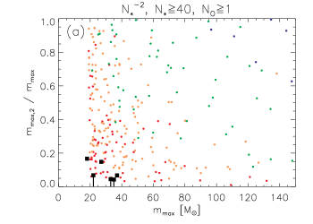
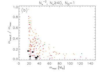
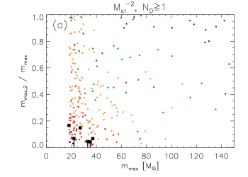
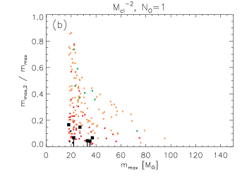
Our observations lie in an interesting region of the parameter space in both the and simulations. There is a strong drop-off in the population of simulated clusters having . This drop-off coincides with some of our observed isolated targets. Thus, the upper limits in for the isolated stars approach the extreme lower limit of the parameter space. All of our observations lie within the parameter space covered by simulated clusters.
To examine this quantitatively, we identify the subset of simulated clusters that correspond to the selection criteria of our observed stars and clusters. For each target star, we identify all simulated clusters having within the uncertainty of the star’s empirically-derived mass (Table 1). We also eliminate all simulated clusters containing more than one O star, to obtain our final sub-sample of simulated clusters. For , we use the mass of the most massive observed, companion main-sequence star. In the case of our apparently isolated massive stars, we set to an upper-limit value of , our F814W completeness limit. In the following analysis, we denote the observed as and that from simulated clusters as . Table 7 lists the fraction of clusters with [ for each star. Column 1 lists the star ID; column 2 lists the mass of the OB star from Table 1; column 3 lists ; columns 4, 5, and 6 list the fraction of clusters with [ for the simulations with , having slopes of –1.8, –2, and –2.3, respectively; and columns 7, 8, and 9 list these fractions for the simulations with , as shown. Columns 5 and 8 correspond to the simulated population in Figures 7b and 8b, respectively. Columns 10 and 11 are the same as Columns 5 and 8, respectively, except that they correspond to the simulated population in Figures 7a and 8a, showing all clusters with O star.
| Star | () | ()obs | , | , | ||||||
|---|---|---|---|---|---|---|---|---|---|---|
| AzV 58 | 22 | 0.07 | 0.01 | 0.02 | 0.03 | 0.04 | 0.06 | 0.09 | 0.02 | 0.05 |
| AzV 67 | 37 | 0.07 | 0.07 | 0.10 | 0.11 | 0.08 | 0.10 | 0.11 | 0.07 | 0.06 |
| AzV 106 | 18 | 0.17 | 0.11 | 0.14 | 0.18 | 0.16 | 0.21 | 0.27 | 0.14 | 0.20 |
| AzV 186 | 33 | 0.05 | 0.01 | 0.02 | 0.02 | 0.03 | 0.04 | 0.05 | 0.01 | 0.03 |
| AzV 226 | 35 | 0.04 | 0.01 | 0.02 | 0.02 | 0.03 | 0.04 | 0.05 | 0.01 | 0.03 |
| AzV 302 | 27 | 0.15 | 0.20 | 0.24 | 0.29 | 0.19 | 0.24 | 0.30 | 0.19 | 0.19 |
Two trends emerge from these data: (1) steepening the power law slope increases the fraction of simulated clusters with [ and (2) the simulations typically have a slightly lower fraction of simulated clusters having [ than the simulations. The first effect is caused by steeper slopes creating a greater fraction of small clusters, where stochastic effects can result in massive stars forming with only a few low mass companions. The second effect is caused by the fact that some of the clusters fall into the low regime in the simulation where , which is not allowed in the simulation, due to our lower limit of . Looking specifically at the simulations, Table 7 shows that the frequency of single O star simulated clusters having [ for all observed groups is below the 25th percentile in both simulations, confirming the impression from Figures 7b and 8b. For all O star clusters from Figures 7a and 8a, our observed groups are all below the 20th percentile. Some of our isolated star observations are found in the lowest 5th percentile in both simulations, but still within the parameter space covered by the simulations.
That our observations are not well-distributed among the cluster population in Figures 7b and 8b is primarily due to our sample selection. Our selection process included a visual inspection of our targets using ground-based imaging to ensure they appeared isolated, thereby ensuring that our objects have extremely low values of . These targets were drawn to qualify for both the field O star and field OB star samples from Oey et al. (2004), defined to have no other stars having and within a clustering length, respectively. Thus by definition, for our sample. On the other hand, 27 of the 91 stars (30%) in the field O star sample of Oey et al. are not members of the field OB sample, implying that for these stars . The remaining 70% of isolated O stars having companions with masses below can be compared to a simulated fraction of 57% in our simulation and 64% in our simulation. However, the SMC field O star sample is contaminated by runaway stars which will inflate the observed fraction of O stars with .
However, we also note that the distribution of in the simulations does depends somewhat on the cluster population parameters and populating algorithm. For example, if we do not discard and repopulate clusters when the total cluster mass exceeds 105% of the target mass (see §3.2), then our test simulations show that the increased production of massive stars can affect the percentiles by up to a factor of two, so that our objects fall in the lowest 50th percentile, for the default simulation. Thus in this case, our observed clusters are nearer to the median and more well-distributed overall.
5. The relation between and
5.1. Observations and Simulations
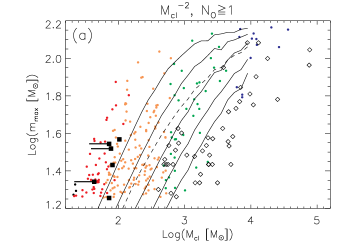
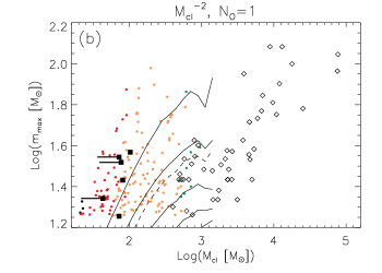
In Figures 9 and 10, we compare the relationship between the cluster mass and maximum stellar mass . As in Figure 7, panel (a) includes simulated clusters with O star, while panel (b) includes only simulated clusters with exactly one O star. The color coding scheme is also the same as in Figure 7. The solid lines show contours for the 10th, 25th, 50th, 75th, and 90th percentiles of as a function of in the simulation, while the dashed line represents the mean. These percentiles are computed from a much larger set of ( simulations) or ( simulations) modeled clusters, to reduce stochastic scatter. For our observations (black squares), we calculate as described in §3.1 (Table 4). The diamonds show observed Galactic clusters whose and are tabulated by Weidner et al. (2010a).
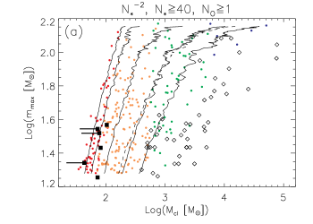
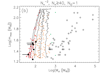
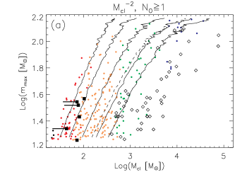
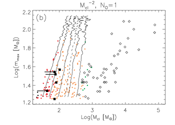
Figures 9a and 10a show that the majority of the Galactic cluster sample lies above the 90th percentile in for a given in both the and simulations. In contrast, our observed objects all occur below the 50th percentile in both simulations and are more representative of the single O star cluster sample in Figures 9b and 10b. Indeed, Figures 9b and 10b show that the majority of the Galactic cluster sample lies outside the single O star cluster parameter space. This indicates that the Galactic cluster sample is comprised of clusters with a well-populated IMF, probably due to selection effects, since more fully populated clusters preferentially tend to be observed (Maschberger & Clarke 2008).
In Figure 11, we plot the mean value as a function of (dashed line) for our simulation. The solid lines now show contours for the 10th, 25th, 50th, 75th, and 90th percentiles of as a function of in the simulation, again calculated from the larger sets of simulated clusters. The dashed line represents the mean. We note that in Figure 11a, the percentiles are calculated from all clusters having a given , while the simulated clusters plotted here are only those which contain at least one O star. In Figure 11b, the percentiles exclude all clusters with multiple O stars, and the plotted clusters are those with a single O star.
Here, we see that nearly all of our observed clusters are above the 90th percentile of as a function of . In Figure 11a, all the Galactic clusters are below the 50th percentile, with the majority below the 10th percentile. Figure 11b again demonstrates that the Galactic O star cluster sample largely falls outside the parameter space of the single O star clusters. Comparing the percentiles plotted in Figure 11b with those in Figure 11a shows little difference for our observed values; however, as increases, the transition from single O star clusters to clusters with O star is revealed in the turnover of the percentiles in Figure 11b. This confirms that the Galactic cluster sample is comprised mainly of clusters with multiple O stars.
5.2. Does determine ?
We now compare our observations with numerical simulations that are limited by a relation between the maximum stellar mass within a cluster and total cluster mass (-). As mentioned in §1, various forms of this relation have been proposed, based on both theory (Bonnell et al. 2004) and observations (WK06), that invoke a physical relation between and . This is different from the purely statistical relation between the average and (Oey & Clarke 2005). In the latter case it is simply improbable to form a massive star in a small cluster, whereas in the integrated galaxial initial mass function (IGIMF) proposed by Weidner & Kroupa (2005), the - relation is modeled deterministically, such that never exceeds the value derived from this - relation. For reference, see Figure 1 of Weidner & Kroupa (2005), which plots various - relations from the literature.
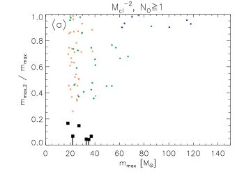
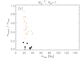
If we adopt the mean in Figure 11a as a simple - relation, then all simulated clusters above the dashed line are in violation of such a relation. We note that the mean corresponds to somewhat lower-mass clusters for a given than the WK06 - relation. Even so, our observed minimal O star groups do not fit within the framework of a steepened IGIMF as presented by Weidner & Kroupa (2005), although we note that statistical variation of the - relation is not included in their work.
Figure 12 shows as a function of for clusters that correspond to our imposed - relation, which are those below the mean plotted in Figure 11a. The color coding and panel samples are the same as in Figure 8. Figure 12a illustrates that all simulated O star clusters now exhibit . With this imposed - relation, our observations appear to fall completely outside the parameter space of the simulations in both Figure 12a and 12b, given the number of clusters corresponding to the SMC cluster population. This form of the deterministic - relation is therefore poorly supported by our observations of minimal O star groups.
One possible interpretation of these results is that our observed objects are remnants of clusters affected by “infant weight loss” (e.g., Bastian & Goodwin, 2006). However, even if the objects have been reduced by a factor of a few in or , they would still be discrepant from the Galactic cluster sample of Weidner et al. (2010a). Recent simulations have shown that cluster mass segregation can occur on timescales of 1 Myr for the most massive cluster stars (Allison et al. 2009). Massive stars segregated to the cluster core are unlikely to be evaporated by “infant weight loss”, and so clusters are likely to retain the two most massive stars. Therefore, the observed values are unlikely to be affected by dynamical evaporation. Moreover, “infant weight loss” is associated with the rapid removal of gas, which, however, is still present in the majority of our objects (§2.3). Furthermore, -body simulations of sparse, young clusters by Weidner et al. (2010b) show that % of the cluster’s mass is removed within 5 Myr, suggesting that significant mass loss is relatively unimportant in such objects.
Our results are similar to those found by Maschberger & Clarke (2008), who examined a sample of clusters from the literature using studies that focused on low clustering around high-mass stars. The observations of isolated Herbig Ae/Be stars by Testi et al. (1997, 1999), as well as our observations of isolated OB stars, show that massive stars may form in even the most sparse environments. As we showed above, these observations are not consistent with a strictly-defined, deterministic - relation. At the very least, the minimal OB groups, along with clusters compiled by Weidner et al. (2010a), imply huge deviation from a direct - relation (Figure 11). While a steepened IGIMF will occur even without a - relation, this result has problematic implications for the magnitude of proposed steepening for the IGIMF in aggregate galactic stellar populations (Weidner & Kroupa 2005). In addition, the competitive accretion theory of star formation is also linked to an - relation (Bonnell et al. 2004), although we note that Maschberger et al. (2010) find that competitive accretion simulations are nevertheless able to produce massive field stars of at least . On the other hand, simulations of star formation based on core accretion (e.g., Krumholz et al. 2010) show that under specific cloud conditions, radiative heating can prevent fragmentation, perhaps more directly forming minimal O star groups similar to those observed in this paper.
6. Conclusions
We carried out a SNAP program with HST’s Advanced Camera for Surveys that yielded high resolution observations of eight field OB stars in the SMC. These stars range in spectral type from O7 to B0.5, and in mass from to . Radial velocities for two stars (AzV 223 and smc16) show them to be runaways, and we may expect one or two more to be transverse runaways. There is no evidence of clustering down to a detection limit in three of the six non-runaway cases. The non-runaway, isolated stars (AzV 58, AzV 186, and AzV 226) remain candidates for isolated OB star formation. Two of these isolated OB stars reside within HII regions, indicating that these stars may still be located in the region of their formation, and strengthening the possibility that these O stars have formed alone. For the other three non-runaway OB stars (AzV 67, AzV 106, and AzV 302), we detect an associated population of stars using a stellar density analysis and a separate friends-of-friends algorithm. After accounting for field contamination, we find eight to ten stars associated with each OB star, ranging in mass from our lower detection limit of to .
The three observations that do show evidence of clustering exhibit a flat IMF with slope of to when combining their populations, although due to the small sample size, the IMF may be consistent with a Salpeter IMF, which has = -1.35. The flat IMF is due to a lack of low-mass companions that ordinarily are expected to form along with these O stars.
Assuming that each of our non-runaway stars is still in the location where it formed, we infer cluster membership of based upon the companion population , integrated over the full stellar mass range for our Kroupa IMF of . Given their inferred , we calculate that a small fraction, only 0.01–0.2, of clusters will form a star with mass observed.
We have conducted Monte Carlo simulations to explore where our observations fall within the cluster parameter space of typical star formation, assuming a Kroupa IMF and either a clustering law based on or cluster mass function based on . The power law slopes and lower limits of and for these simulations were constrained using observations of massive star clustering in the SMC by Oey et al. (2004) and the fraction of isolated Galactic O stars by de Wit et al. (2005). Together, these observational constraints resulted in a –2 power law slope with lower limits of = 40 or as the best fit models, which we adopted as the default simulations for this study. These default and models match equally well with the observations, thus neither one is established as a more suitable metric for modeling cluster distribution.
We find that observed mass ratios of the two highest-mass stars are below the 25th percentile of single O star clusters generated by the default simulations. This result is due to choosing targets which appeared isolated in ground-based imaging. Our observations also lie below the 50th percentile when comparing total cluster mass (either or ) as a function of , whereas a sample of Galactic clusters from Weidner et al. (2010a) are nearly all above the 90th percentile. These numbers suggest that our observations are more typical examples of O star clusters than the Galactic cluster sample, which contains clusters with well-populated IMFs.
We show evidence that our observed minimal O star groups are inconsistent with a deterministic - relation. By extension, our observations are also inconsistent with the - relation proposed for the IGIMF effect (Weidner & Kroupa 2005) and the relation that (Bonnell et al. 2004), predicted by the competitive accretion model of massive star formation. We argue that in most cases, an observed - relation is simply a product of the stochastic, probabilistic nature of a universal IMF, rather than an IMF with a variable upper limit corresponding to cluster mass. We conclude that our observations of minimal O star groups are consistent with a universal stellar mass function, including a constant stellar upper-mass limit, without the need to invoke a - relation.
References
- Allison et al. (2009) Allison, R. J., Goodwin, S. P., Parker, R. J., de Grijs, R., Portegies Zwart, S. F., & Kouwenhoven, M. B. N. 2009, ApJ, 700, L99
- Azzopardi et al. (1975) Azzopardi, M., Vigneau, J., & Macquet, M. 1975, A&AS, 22, 285
- Bastian & Goodwin (2006) Bastian, N., & Goodwin, S. P. 2006, MNRAS, 369, L9
- Battinelli (1991) Battinelli, P. 1991, A&A, 244, 69
- Blaauw (1961) Blaauw, A. 1961, Bull. Astron. Inst. Netherlands, 15, 265
- Bonnell et al. (2001) Bonnell, I. A., Bate, M. R., Clarke, C. J., & Pringle, J. E. 2001, MNRAS, 323, 785
- Bonnell et al. (2003) Bonnell, I. A., Bate, M. R., & Vine, S. G. 2003, MNRAS, 343, 413
- Bonnell & Clarke (1999) Bonnell, I. A., & Clarke, C. J. 1999, MNRAS, 309, 461
- Bonnell et al. (2008) Bonnell, I. A., Clark, P., & Bate, M. R. 2008, MNRAS, 389, 1556
- Bonnell et al. (2007) Bonnell, I. A., Larson, R. B., & Zinnecker, H. 2007, Protostars and Planets V, 149
- Bonnell et al. (2004) Bonnell, I. A., Vine, S. G., & Bate, M. R. 2004, MNRAS, 349, 735
- Chandar et al. (2010) Chandar, R., Fall, S. M., & Whitmore, B. C. 2010, ApJ, 711, 1263
- Charbonnel et al. (1993) Charbonnel, C., Meynet, G., Maeder, A., Schaller, G., & Schaerer, D. 1993, A&AS, 101, 415
- Crowther (1997) Crowther, P. A. 1997, IAU Symposium, 189, 137
- de Wit et al. (2004) de Wit, W. J., Testi, L., Palla, F., Vanzi, L., & Zinnecker, H. 2004, A&A, 425, 937
- de Wit et al. (2005) de Wit, W. J., Testi, L., Palla, F., & Zinnecker, H. 2005, A&A, 437, 247
- Elmegreen (2000) Elmegreen, B. G. 2000, ApJ, 530, 277
- Elmegreen (2006) Elmegreen, B. G. 2006, ApJ, 648, 572
- Elmegreen (2008) Elmegreen, B. G. 2008, ApJ, 672, 1006
- Evans et al. (2006) Evans, C. J., Lennon, D. J., Smartt, S. J., & Trundle, C. 2006, A&A, 456, 623
- Gieles (2009) Gieles, M. 2009, MNRAS, 394, 2113
- Gies (1987) Gies, D. R. 1987, ApJS, 64, 545
- Girardi et al. (2002) Girardi, L., Bertelli, G., Bressan, A., Chiosi, C., Groenewegen, M. A. T., Marigo, P., Salasnich, B., & Weiss, A. 2002, A&A, 391, 195
- Haas & Anders (2010) Haas, M. R., & Anders, P. 2010, A&A, 512, A79
- Harries et al. (2003) Harries, T. J., Hilditch, R. W., & Howarth, I. D. 2003, MNRAS, 339, 157
- Harris & Pudritz (1994) Harris, W. E., & Pudritz, R. E. 1994, ApJ, 429, 177
- Hoogerwerf et al. (2001) Hoogerwerf, R., de Bruijne, J. H. J., & de Zeeuw, P. T. 2001, A&A, 365, 49
- Hoversten & Glazebrook (2008) Hoversten, E. A., & Glazebrook, K. 2008, ApJ, 675, 163
- Hunter et al. (2003) Hunter, D. A., Elmegreen, B. G., Dupuy, T. J., & Mortonson, M. 2003, AJ, 126, 1836
- Köppen et al. (2007) Köppen, J., Weidner, C., & Kroupa, P. 2007, MNRAS, 375, 673
- Kroupa (2001) Kroupa, P. 2001, MNRAS, 322, 231
- Kroupa & Weidner (2003) Kroupa, P., & Weidner, C. 2003, ApJ, 598, 1076
- Krumholz et al. (2010) Krumholz, M. R., Cunningham, A. J., Klein, R. I., & McKee, C. F. 2010, ApJ, 713, 1120
- Krumholz et al. (2009) Krumholz, M. R., Klein, R. I., McKee, C. F., Offner, S. S. R., & Cunningham, A. J. 2009, Science, 323, 754
- Krumholz & McKee (2008) Krumholz, M. R., & McKee, C. F. 2008, Nature, 451, 1082
- Lee et al. (2009) Lee, J. C., et al. 2009, ApJ, 706, 599
- Li et al. (2003) Li, Y., Klessen, R. S., & Mac Low, M.-M. 2003, ApJ, 592, 975
- Maschberger & Clarke (2008) Maschberger, T., & Clarke, C. J. 2008, MNRAS, 391, 711
- Maschberger et al. (2010) Maschberger, T., Clarke, C. J., Bonnell, I. A., & Kroupa, P. 2010, MNRAS, 404, 1061
- Massey (2002) Massey, P. 2002, ApJS, 141, 81
- Massey et al. (1995) Massey, P., Lang, C. C., Degioia-Eastwood, K., & Garmany, C. D. 1995, ApJ, 438, 188
- Massey et al. (2005) Massey, P., Puls, J., Pauldrach, A. W. A., Bresolin, F., Kudritzki, R. P., & Simon, T. 2005, ApJ, 627, 477
- Massey et al. (2009) Massey, P., Zangari, A. M., Morrell, N. I., Puls, J., DeGioia-Eastwood, K., Bresolin, F., & Kudritzki, R.-P. 2009, ApJ, 692, 618
- Meurer et al. (2009) Meurer, G. R., et al. 2009, ApJ, 695, 765
- Meurer et al. (1995) Meurer, G. R., Heckman, T. M., Leitherer, C., Kinney, A., Robert, C., & Garnett, D. R. 1995, AJ, 110, 2665
- Oey & Clarke (1998) Oey, M. S., & Clarke, C. J. 1998, AJ, 115, 1543
- Oey & Clarke (2005) Oey, M. S., & Clarke, C. J. 2005, ApJ, 620, L43
- Oey et al. (2004) Oey, M. S., King, N. L., & Parker, J. W. 2004, AJ, 127, 1632
- Oey et al. (2003) Oey, M. S., Parker, J. S., Mikles, V. J., & Zhang, X. 2003, AJ, 126, 2317
- Parker & Goodwin (2007) Parker, R. J., & Goodwin, S. P. 2007, MNRAS, 380, 1271
- Pflamm-Altenburg et al. (2009) Pflamm-Altenburg, J., Weidner, C., & Kroupa, P. 2009, MNRAS, 395, 394
- Rosolowsky (2005) Rosolowsky, E. 2005, PASP, 117, 1403
- Scalo (1986) Scalo, J. M. 1986, Fund. Cosmic Phys., 11, 1
- Selman & Melnick (2008) Selman, F. J., & Melnick, J. 2008, ApJ, 689, 816
- Sirianni et al. (2005) Sirianni, M., et al. 2005, PASP, 117, 1049
- Smith et al. (2000) Smith, C., Leiton, R., & Pizarro, S. 2000, Stars, Gas and Dust in Galaxies: Exploring the Links, 221, 83
- Shu et al. (1987) Shu, F. H., Adams, F. C., & Lizano, S. 1987, ARA&A, 25, 23
- Spaans & Silk (2000) Spaans, M., & Silk, J. 2000, ApJ, 538, 115
- Stanimirović et al. (2004) Stanimirović, S., Staveley-Smith, L., & Jones, P. A. 2004, ApJ, 604, 176
- Staveley-Smith et al. (1997) Staveley-Smith, L., Sault, R. J., Hatzidimitriou, D., Kesteven, M. J., & McConnell, D. 1997, MNRAS, 289, 225
- Testi et al. (1999) Testi, L., Palla, F., & Natta, A. 1999, A&A, 342, 515
- Testi et al. (1997) Testi, L., Palla, F., Prusti, T., Natta, A., & Maltagliati, S. 1997, A&A, 320, 159
- Thilker et al. (2007) Thilker, D. A., et al. 2007, ApJS, 173, 538
- Udalski et al. (1998) Udalski, A., Szymanski, M., Kubiak, M., Pietrzynski, G., Wozniak, P., & Zebrun, K. 1998, Acta Astronomica, 48, 147
- Weidner et al. (2010) Weidner, C., Bonnell, I. A., & Moeckel, N. 2010, arXiv:1008.4578
- Weidner & Kroupa (2004) Weidner, C., & Kroupa, P. 2004, MNRAS, 348, 187
- Weidner & Kroupa (2005) Weidner, C., & Kroupa, P. 2005, ApJ, 625, 754
- Weidner & Kroupa (2006) Weidner, C., & Kroupa, P. 2006, MNRAS, 365, 1333
- Weidner et al. (2010) Weidner, C., Kroupa, P., & Bonnell, I. A. D. 2010, MNRAS, 401, 275
- Zaritsky et al. (2002) Zaritsky, D., Harris, J., Thompson, I. B., Grebel, E. K., & Massey, P. 2002, AJ, 123, 855
- Zhang & Fall (1999) Zhang, Q., & Fall, S. M. 1999, ApJ, 527, L81
- Zinnecker (1982) Zinnecker, H. 1982, Annals of the New York Academy of Sciences , 395, 226