Correlated couplings and robustness of coupled networks
Abstract
Most real-world complex systems can be modelled by coupled networks with multiple layers. How and to what extent the pattern of couplings between network layers may influence the interlaced structure and function of coupled networks are not clearly understood. Here we study the impact of correlated inter-layer couplings on the network robustness of coupled networks using percolation concept. We found that the positive correlated inter-layer coupling enhances network robustness in the sense that it lowers the percolation threshold of the interlaced network than the negative correlated coupling case. At the same time, however, positive inter-layer correlation leads to smaller giant component size in the well-connected region, suggesting potential disadvantage for network connectivity, as demonstrated also with some real-world coupled network strucutres.
pacs:
89.75.Hc, 89.75.FbIn the past decade, network has proved to be a useful framework to model structural complexity of complex systems small ; scale . By abstracting a complex system into nodes (constituents) and links (interactions between them), the resulting graph could be efficiently treated analytically and numerically, through which a large body of new physics of complex systems has been acquired caldarelli-book ; havlin-book . Most studies until recently have focused on the properties of isolated, single networks, such as the World wide web, coauthorship network of a specific subject, and the metabolic network of a microorganism. In most, if not all, situations, however, a network in question is merely a part of a larger system; world wide web could only function properly in conjuction with physical network of routers, a researcher could take part in multiple social networks via various professional or informal relationships other than coauthorship relations, and a protein in a cell could function both as a metabolic enzyme and by binding with other proteins, thereby taking part in both metabolic and protein networks. Therefore, a more complete description of complex systems would be a system of networks coupled one another. Typical forms of network coupling would be layered structure kurant , multiplexity of links multiplexity , and interaction leicht or interdependency buldyrev between network layers.
Only recently, such coupled network structures have started to be studied actively leicht ; buldyrev ; more ; buldyrev2 . Leicht and D’Souza leicht studied what they called interacting networks, in which two networks are coupled via inter-network edges, and developed a generating function formalism to study their percolation properties. Buldyrev et al. buldyrev studied the interdependent networks, in which mutual connectivity in two network layers plays an important role, and found that catastrophic cascades of failure generically occur due to the interdependency. In both studies, network layers are coupled in an uncorrelated way, in the sense that the connections or pairings between nodes in different layers are taken to be random. In real complex systems, however, correlated inter-layer couplings can be siginificant. For example, one may expect that a person with many friends in one social network would also have many friends in another social network, being a friendly person. Such correlated coupling may alter the interlaced connectivity structure and large-scale properties of dynamic processes on the coupled networks, such as network robustness cohen or cascading failures buldyrev ; buldyrev2 ; goh . Therefore, the impact of correlated inter-layer coupling to system’s structure and function needs to be understood.
In this paper, we study how the network robustness is affected by the correlated inter-layer coupling in two-layer coupled networks. Specifically, we consider two networks with identical set of nodes. They can be individuals participating in two different social networks or proteins with activities via enzymes and multi-protein assembly. Each layer is specificed with the intra-layer degree distribution , where degree is the number of links within layer (intra-layer links) of the node. The coupled network can be specified by the joint degree distribution . Generalization into layers is straightforward, and in this study we restrict ourselves to case. Next the network layers are overlaid one another, and the interlaced network is constructed. The degree of a node in the interlaced network is given by , where denotes the number of links overlapping in the two layers, which can be neglected in sparse networks. Therefore, the generating function for the degree distribution of the interlaced network can be written as
| (1) |
The primary quantity of interest is the size of giant component of the interlaced network, given by the fraction of nodes belonging to the largest component in the limit . Following standard generating function technique newman , can be obtained via
| (2) |
with being the solution of , where is the generating function of the probability distribution of remaing degrees . The condition for existence of the giant component (that is, ) is given by the Molloy-Reed criterion molloy , . Therefore, understanding of how the inter-layer coupling correlation encoded in the joint degree distribution translates into the degree distribution of the interlaced network can provide critical insight on network robustness.
In the absence of inter-layer correlations, the joint degree distribution factorizes, , and therefore the degree distribution of the interlaced network is given by the convolution of , , and its generating function , where is the generating function of . In the presence of inter-layer correlations, however, is related with in a nontrivial way.
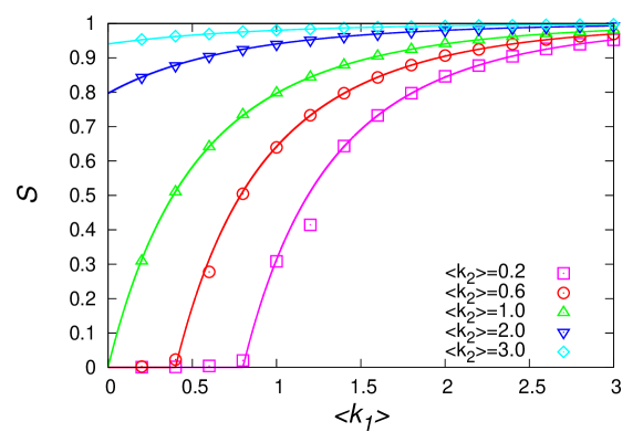
To gain more insight, we consider specific network models. First we consider two layers of Erdős-Rényi (ER) networks with mean degrees and , respectively. For the uncorrelated case, one can proceed with exact calculations as , from which can be obtained using Eq. (2). The interlaced network is nothing but another ER network with mean degree . Numerical simulations with two-layer ER networks with perfectly confirmed this theoretical prediction (Fig. 1). Percolation transition occurs when .
Next we introduce the correlated inter-layer coupling in the two-layer networks. For simplicity, we consider two extreme cases of maximally-positive and maximally-negative correlations. In the maximally-positive inter-layer correlation, the ranks in degrees of a node in the two layers are equal, meaning that the highest degree node in one layer is also the highest degree node in the other layer, and similarly for the lowest degree nodes. Specifically, the Spearman rank correlation coefficient of the degrees of a node, defined by
| (3) |
where is the difference in the ranks of node ’s degrees in the two layers, is . In the maximally-negative case, it is the opposite that the highest degree node in one layer has the lowest degree in the other layer, having the reverse ordering of ranks. In this case, the rank correlation coefficient is foot .
To construct the networks with maximal correlations, we arrange the nodes in the order of their degrees in each layer and match two nodes from each layer in order of the degree-rank (maximally-positive) or in the opposite order of the degree-rank (maximally-negative). We performed numerical simulations following this procedure for the two-layer ER networks and measured the size of giant component as a function of with fixed (Fig. 2, points). We also performed the following mean-field-like numerical calculations for for both cases and used them to obtain through Eqs. (1-2), which are found to agree with the numerical simulation results remarkably well (Fig. 2, lines). For maximally-positive case, we setup two ordered sequences obtained from the cumulative intra-layer degree distribution, , of each layer , and merge them to make another ordered sequence. This sequence is nothing but the cumulative distribution of , from which we can calculate easily. For maximally-negative case, we need to use two ordered sequences given by the cumulative degree distribution in one layer and the complementary cumulative degree distribution, , in the other layer.
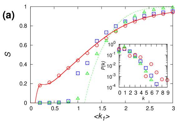
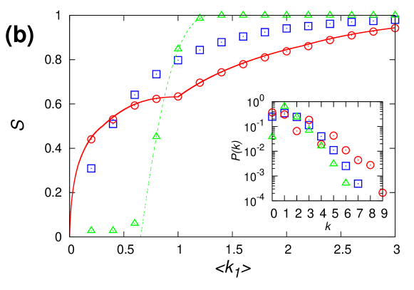
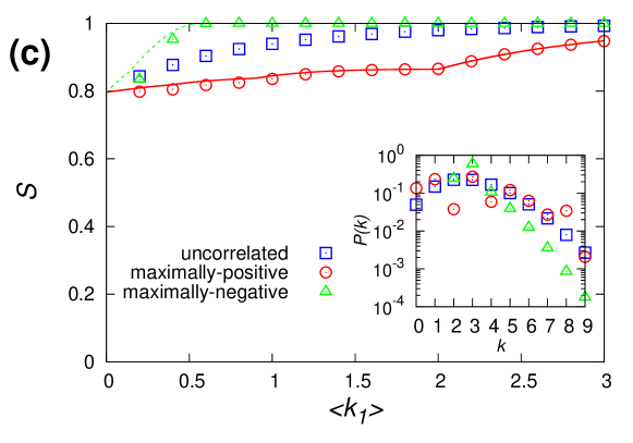
Both numerical simulations and mean-field-like calculations show that in the maximally-positive case, the giant component emerges much earlier than in the uncorrelated case. For example, with [Fig. 2(a)], which is well below the percolation threshold of a single ER network, the giant component emerges at as early as (), much earlier than the uncorrelated case where it does at (). This means that we only need less than a third of links ( vs. ) to attain global connectivity in the maximally-positive case with , compared with the uncorrelated case. By contrast, in the maximally-negative case, the giant component emerges much later. For example, with [Fig. 2(b)], exactly the percolation threshold of a single ER network, the giant component does not grow to a finite size until (), that is, at , meaning that, surprisingly, additions of about two thirds more links onto the giant component at the single network percolation point do not make it grow any larger. Therefore we need much more links to attain global connectivity in the maximally-negative case compared with the uncorrelated case. In this sense, the positive coupling between layers renders the coupled network more robust under random failures, whereas the negative coupling decreases the robustness. These distinct behaviors arise due to the different shapes of degree distribution in each case. For positive correlation case, the degree distribution becomes broader than the uncorrelated case, whereas it gets narrower in the negative correlation case, leading to smaller degree variance (Fig. 2, insets).
Although the giant component emerges earlier with positive inter-layer coupling, it grows more gradually than the negative correlation case, for which it exhibits a more abrupt increase near the percolation threshold and faster saturation towards (Fig. 2). This suggests an interesting perspective to network robustness; on one hand, the coupled network with positive inter-layer correlations is more robust since it can support global connectivity with lower density of links, whereas on the other hand, the early impact of link removals from a well-connected network can be more severe, as is smaller for the positive correlation case than for the negative correlation case in the region . This behavior can also be seen in Fig. 2(c), where the giant component size is plotted against with , well above the percolation threshold. In this case, the maximally-negative correlation case exhibits larger than the maximally-positive case in the whole range of we studied. These results are somewhat similar to the effect of degree mixing pattern in the single network assortative .
We performed the same calculations for coupled networks with two layers of scale-free (SF) networks having identical degree distributions of a power-law form, , with the degree exponent and using the static model static , and obtained qualitatively same results.
Finally, we consider real-world examples of coupled network structures. The first example is the cellular network of a bacterium called Mycoplasma pneumoniae pneumonia , in which nodes are genes or gene products and links are the physical bindings to form protein assemblies in the protein-protein interaction layer and the sharing of metabolites in reactions catalyzed by two enzymes in the metabolic layer. The second example is the world trade network wtn ; garlaschelli , in which the nodes are countries and links are trade relations between them, with two layers corresponding to commodity trades in the primary and the secondary industrial sectors, respectively.
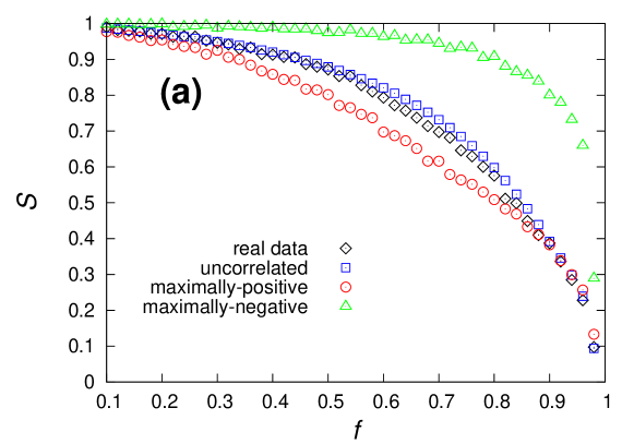
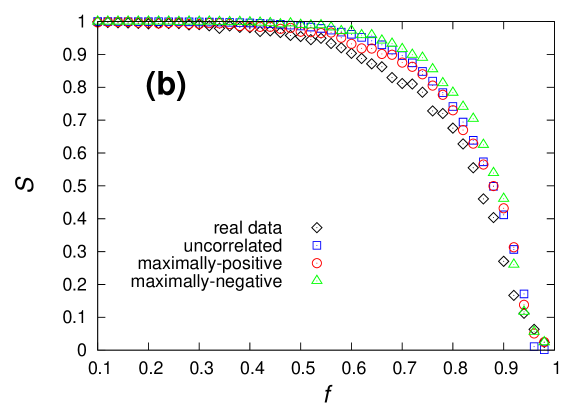
We studied the robustness properties of these coupled networks under random failures by successively removing links randomly. In particular we measured the giant component size as a function of the fraction of links removed for the interlaced networks (Fig. 3, ). We compared the results with the randomized coupled networks by randomly shuffling the node identities in the two layers with the intra-layer connectivity intact, by which we could obtain the uncorrelated coupled networks (Fig. 3, ). Furthermore, we constructed the maximally-positive (Fig. 3, ) and maximally-negative (Fig. 3, ) correlated coupled networks, by ordered-matching and anti-ordered-matching of degree ranks in the two layers as in the model networks. As both real-world networks have broad intra-layer degree distributions, often of a power-law form with , both the coupled networks show extreme resilience under random failures, that is the giant component sustains () until we remove almost the entire links (). Distinct characteristics, however, can be observed when we compare them with corresponding randomized networks. The cellular network of M. pneumoniae behaves similarly to the uncorrelated randomized networks [Fig. 3(a)], whereas the world trade network behaves closely to the maximally-positive correlated case [Fig. 3(b)], suggesting a fundamental difference in the inter-layer coupling structure in these two systems. Indeed, the inter-layer degree rank correlation is measured to be weak for the former, , whereas it is found to be very strongly positive for the latter, , consistent with expectations based on the model network results.
To conclude, we have studied the effect of correlated inter-layer couplings on the network robustness of coupled network structures, using both model networks and real-world networks. It is shown that the positive inter-layer correlation in degrees renders the network robustness increase in the sense that the percolation threshold is lowered. At the same time, the giant component, once formed, grows much more gradually, or equivalently, decays much quickly under initial random link removal, for positive inter-layer correlations, which has an important implication for real-world networks with scale-free topology. We have shown that the correlated coupling between network layers affects critically the structural properties of coupled network system, a better representation of most real-world complex systems than the single, isolated network. Its impact on other dynamic processes occurring on coupled network systems is to be explored buldyrev2 . Finally, higher-order correlation factors within and between network layers, such as link overlaps, mixing, clustering, and community patterns, could also induce other nontrivial impact on coupled network structure and dynamics, opening a wide avenue for future studies.
Acknowledgements.
We thank J. Choi and K.-M. Lee for their help with real-world network data. This work was supported by Mid-career Researcher Program through NRF grant funded by the MEST (No. 2009-0080801). While finalizing the manuscript, we learned of an independent study by Parshani et al. inter-similarity which dealt with a similar problem on interdependent networks and obtained results partly overlapping with ours.References
- (1) D. J. Watts and S. H. Strogatz, Nature (London) 393, 440 (1998).
- (2) A.-L. Barabási and R. Albert, Science 286, 509 (1999).
- (3) G. Caldarelli, Scale-free networks (Oxford University Press, Oxford, 2007).
- (4) S. Havlin and R. Cohen, Complex neworks: Structure, robustness and function (Cambridge Unviersity Press, Cambridge, 2010).
- (5) M. Kurant and P. Thiran, Phys. Rev. Lett. 96, 138701 (2006).
- (6) S. Wasserman and K. Faust, Social network analysis (Cambridge University Press, Cambridge, 1994).
- (7) E. A. Leicht and R. M. D’Souza, arXiv:0907.0894.
- (8) S. V. Buldyrev, et al., Nature (London) 464, 1025 (2010).
- (9) S. Funk and V. A. A. Jansen, Phys. Rev. E 81, 036118 (2010); R. Parshani, S. V. Buldyrev, and S. Havlin, Phys. Rev. Lett. 105, 048701 (2010); C. D. Brummitt, R. M. D’Souza, and E. A. Leicht, arXiv:1010.0279.
- (10) S. V. Buldyrev, N. Shere, and G. A. Cwilich, arXiv:1009.3183.
- (11) R. Cohen, K. Erez, D. ben-Avraham, and S. Havlin, Phys. Rev. Lett. 85, 4626 (2000).
- (12) K.-I. Goh, D.-S. Lee, B. Kahng, and D. Kim, Phys. Rev. Lett. 91, 148701 (2003).
- (13) M. E. J. Newman, S. H. Strogatz, and D. J. Watts, Phys. Rev. E 64, 026118 (2001).
- (14) M. Molloy and B. Reed, Rand. Struct. Algorithms 6, 161 (1995).
- (15) becomes strictly or for maximally-correlated cases when there are no ties in the ranks. When there are ties, the average rank is used to compute .
- (16) M. E. J. Newman, Phys. Rev. Lett. 89, 208701 (2002).
- (17) K.-I. Goh, B. Kahng, and D. Kim, Phys. Rev. Lett. 87, 278701 (2001).
- (18) S. Kühner, et al., Science 326, 1235 (2009); E. Yus, et al., ibid. 326, 1263 (2009).
- (19) United Nations COMTRADE Database (http://comtrade.un.org/).
- (20) M. Barigozzi, G. Fagiolo, and D. Garlaschelli, Phys. Rev. E 81, 046104 (2010).
- (21) R. Parshani, et al., arXiv:1010.4506.