An iterative approach for amplitude amplification with nonorthogonal measurements

H. T. Ng1 and Franco Nori1,2 1Advanced Science Institute, RIKEN, Wako-shi, Saitama 351-0198, Japan 2Physics Department, The University of Michigan, Ann Arbor, Michigan 48109-1040, USA
Abstract

Using three coupled harmonic oscillators, we present an amplitude-amplification method for factorization of an integer. We generalize the method in [arXiv:1007.4338] by employing non-orthogonal measurements on the harmonic oscillator. This method can increase the probability of obtaining the factors by repeatedly using the nonlinear interactions between the oscillators and non-orthogonal measurements. However, this approach requires an exponential amount of resources for implementation. Thus, this method cannot provide a speed-up over classical algorithms unless its limitations are resolved.

pacs:
03.67.Ac

I Introduction

Quantum computing based on qubits has attracted considerable attention (see, e.g., Feynman ; Deutsch1 ; Ekert ; Nielsen ; Kaye ; Buluta1 ; Buluta2 ). There are several candidates to realize quantum computers, such as using nuclear spins in molecules, photons, trapped ions, superconducting circuit and quantum dots (see, e.g., Buluta2 ; You ). However, it is still a great challenge to build a large-scale quantum computer.

Quantum computers can significantly outperform classical computers in doing some specific tasks Ekert ; Nielsen ; Kaye ; Childs . For example, two important quantum algorithms are Shor’s Shor and Grover’s Grover . Shor’s algorithm Shor can factorize a large integer in polynomial time, offering an exponential speed-up over classical computation. Grover’s algorithm Grover gives a quadratic speed-up in searching database. This search algorithm has been found to be very useful in other related problems Nielsen ; Kaye ; Childs . To date, the study of quantum algorithms is a very active area of research (see, e.g., Childs ).

Using three coupled harmonic oscillators, we have recently proposed Ng an alternative approach for factoring integers. We consider these three harmonic oscillators to be coupled together via nonlinear interactions Ng . To factorize an integer N𝑁N, this approach involves only three steps: initialization, time evolution, and conditional measurement. In this approach, the states of the first two harmonic oscillators are prepared in a number-state basis, while the state of the third oscillator is prepared in a coherent state. The states of the first two harmonic oscillators encode the trial factors of the number N𝑁N. The nonlinear interactions between the oscillators produce coherent states that simultaneously rotate in phase space with different effective frequencies, which are proportional to the product of two trial factors Ng . In this way, all possible products of any two trial factors can be simultaneously computed, and then they are “written” to the rotation frequencies of the coherent states in a single step. The resulting state of the first two oscillators is the factors’ state Ng by performing a conditional measurement of a coherent state rotating with an effective frequency which is proportional to N𝑁N. However, the probability of obtaining this coherent state becomes low when N𝑁N is large. In this paper, we can circumvent this limitation by using an iterative method for increasing the chance of finding the states of the factors. This amplitude-amplification method involves a number of iterations, where each iteration is very similar to the factoring approach we recently proposed Ng .

Now we briefly describe this amplitude-amplification method for factorization using three coupled harmonic oscillators. Let us now consider the first step of our approach. Initially, the first two harmonic oscillators are in a number-state basis and the third oscillator is in a coherent state. Let the three coupled harmonic oscillators evolve for a period of time. The detection is then conditioned on a coherent state with a rotation frequency being proportional to N𝑁N. The probability of finding this coherent state can be adjusted by choosing both an appropriate period of time evolution and magnitude of the coherent state. Here we find that this probability is not small. Indeed, the probability of finding the factors’ state can be increased by a factor which is the reciprocal of the probability of obtaining this coherent state. But the word ”probability” in these sentences is different to the total probability of obtaining the factors.

The resulting states of the first two oscillators, after the first step, are used as new input states in the second step of our approach. Also, the state of the third oscillator is now prepared as a coherent state with the same, or higher, magnitude. By repeating the same procedure described in the first step, we can obtain the states of the factors with a much higher probability. We then iterate these procedures L(log2N)similar-to𝐿subscript2𝑁L\sim(\log_{2}{N}) times, until the probability of finding the factors’ state is close to one.

As an example of how this method works, we show how to factorize the integer 1,030,189=1009×10211030189100910211,030,189=1009{\times}1021. Here the probabilities of obtaining coherent states, with rotation frequencies proportional to N𝑁N, are larger than 0.1 in each iteration. The probability of finding the factors can reach nearly one after 12 iterations. By comparing with the examples N=101,617𝑁101617N=101,617 and 10,961, we can show that the required number of iterations for factoring logarithmically scales with N𝑁N.

However, this approach requires an exponential amount of resources for its implementation. First, it requires an exponential amount of energy to encode a number N𝑁N onto the state of a harmonic oscillator. The input energy scales with the number N𝑁N. Therefore, the required energy becomes enormous if the number N𝑁N is large. Second, it is necessary to prepare an exponential size O(N)𝑂𝑁O(N) of ensemble of oscillators for this iterative approach. This is because a large number of oscillators are abandoned after a conditional measurement. A number at least of order of O(N)𝑁(N) oscillators are thus required to be prepared for the input size N𝑁N. Therefore, this approach does not provide any speed-up for factorization compared to classical algorithms.

This paper is organized as follows: In section II, we introduce a system of coupled harmonic oscillators. In section III, we study the quantum dynamics of the coupled harmonic oscillators starting with a product state of number states and a coherent state. In section IV, we propose an amplitude-amplification method to factorize an integer using three coupled harmonic oscillators. We discuss the convergence and performance of this factoring algorithm. For example, we show how to factor the number 1,030,18910301891,030,189 using this approach. In section V, we discuss the problems and limitations of this approach. Finally, we make a summary in section VI.

II System

We consider a system of (A+B)𝐴𝐵(A+B) coupled harmonic oscillators. The Hamiltonian of the j𝑗j-th harmonic oscillator is written as

Hoscjsubscriptsuperscript𝐻𝑗osc\displaystyle H^{j}_{\rm osc} =\displaystyle= Pj22mj+mjωjXj22,subscriptsuperscript𝑃2𝑗2subscript𝑚𝑗subscript𝑚𝑗subscript𝜔𝑗subscriptsuperscript𝑋2𝑗2\displaystyle\frac{P^{2}_{j}}{2m_{j}}+\frac{m_{j}\omega_{j}{X^{2}_{j}}}{2}, (1)

where ωjsubscript𝜔𝑗\omega_{j} is the frequency of the harmonic oscillator, mjsubscript𝑚𝑗m_{j} is the mass of the particle, and j=1,,A+B𝑗1𝐴𝐵j=1,\ldots,A+B. The operators Xjsubscript𝑋𝑗X_{j} and Pjsubscript𝑃𝑗P_{j} are the position and momentum operators, which satisfy the commutation relation, [Xj,Pj]=isubscript𝑋𝑗subscript𝑃𝑗𝑖Planck-constant-over-2-pi[X_{j},P_{j}]=i\hbar. The annihilation and creation operators of the j𝑗j-th harmonic oscillator are defined as

ajsubscript𝑎𝑗\displaystyle a_{j} =\displaystyle= mjωj2(Xj+iPjmjωj),subscript𝑚𝑗subscript𝜔𝑗2Planck-constant-over-2-pisubscript𝑋𝑗𝑖subscript𝑃𝑗subscript𝑚𝑗subscript𝜔𝑗\displaystyle\sqrt{\frac{m_{j}\omega_{j}}{2\hbar}}\bigg{(}X_{j}+\frac{iP_{j}}{m_{j}\omega_{j}}\bigg{)}, (2)
ajsubscriptsuperscript𝑎𝑗\displaystyle a^{\dagger}_{j} =\displaystyle= mjωj2(XjiPjmjωj).subscript𝑚𝑗subscript𝜔𝑗2Planck-constant-over-2-pisubscript𝑋𝑗𝑖subscript𝑃𝑗subscript𝑚𝑗subscript𝜔𝑗\displaystyle\sqrt{\frac{m_{j}\omega_{j}}{2\hbar}}\bigg{(}X_{j}-\frac{iP_{j}}{m_{j}\omega_{j}}\bigg{)}. (3)

The operators ajsubscript𝑎𝑗a_{j} and ajsubscriptsuperscript𝑎𝑗a^{\dagger}_{j} obey the commutator [aj,aj]=1subscript𝑎𝑗subscriptsuperscript𝑎𝑗1[a_{j},a^{\dagger}_{j}]=1. The Hamiltonian of the three harmonic oscillators can be expressed in terms of the annihilation and creation operators:

H0=j=1A+Bωjajaj,subscript𝐻0Planck-constant-over-2-pisubscriptsuperscript𝐴𝐵𝑗1subscript𝜔𝑗subscriptsuperscript𝑎𝑗subscript𝑎𝑗H_{0}=\hbar\sum^{A+B}_{j=1}{\omega_{j}}a^{\dagger}_{j}a_{j}, (4)

Here we have ignored the constant term.

We consider the harmonic oscillators coupled to each other via nonlinear interactions Ng . Such nonlinear interactions can be described by the Hamiltonian HIsubscript𝐻𝐼H_{I} as

HI=k=A+1A+Bfk(n1,,nA)akaksubscript𝐻𝐼Planck-constant-over-2-pisubscriptsuperscript𝐴𝐵𝑘𝐴1subscript𝑓𝑘subscript𝑛1subscript𝑛𝐴subscriptsuperscript𝑎𝑘subscript𝑎𝑘H_{I}={\hbar}\sum^{A+B}_{k=A+1}f_{k}(n_{1},\ldots,n_{A})a^{\dagger}_{k}a_{k}\\ (5)

where fk(n1,,nA)subscript𝑓𝑘subscript𝑛1subscript𝑛𝐴f_{k}(n_{1},\ldots,n_{A}) are linear or nonlinear-operator functions (excluding divisions) of the number operators nj=ajajsubscript𝑛𝑗subscriptsuperscript𝑎𝑗subscript𝑎𝑗n_{j}=a^{\dagger}_{j}a_{j}, for j=1,,A𝑗1𝐴j=1,\ldots,{A}, and k=A+1,,A+B𝑘𝐴1𝐴𝐵k=A+1,\ldots,{A+B}.

The total Hamiltonian H=H0+HI𝐻subscript𝐻0subscript𝐻𝐼H=H_{0}+H_{I} can be written as

H=j=1A+Bωjajaj+k=A+1A+Bfk(n1,,nA)akak.𝐻Planck-constant-over-2-pisubscriptsuperscript𝐴𝐵𝑗1subscript𝜔𝑗subscriptsuperscript𝑎𝑗subscript𝑎𝑗Planck-constant-over-2-pisubscriptsuperscript𝐴𝐵𝑘𝐴1subscript𝑓𝑘subscript𝑛1subscript𝑛𝐴subscriptsuperscript𝑎𝑘subscript𝑎𝑘H=\hbar\sum^{A+B}_{j=1}{\omega_{j}}a^{\dagger}_{j}a_{j}+{\hbar}\sum^{A+B}_{k=A+1}f_{k}(n_{1},\ldots,n_{A})a^{\dagger}_{k}a_{k}. (6)

The Hamiltonians H0subscript𝐻0H_{0} and HIsubscript𝐻𝐼H_{I} commute with each other, i.e, [H0,HI]=0subscript𝐻0subscript𝐻𝐼0{[H_{0},H_{I}]}=0. The total Hamiltonian H𝐻H in Eq. (6) is exactly solvable. The eigenstate |Em1,,mA+Bketsubscript𝐸subscript𝑚1subscript𝑚𝐴𝐵|E_{m_{1},\ldots,m_{A+B}}\rangle of the Hamiltonian H𝐻H is a product state of number states |mjjsubscriptketsubscript𝑚𝑗𝑗|m_{j}\rangle_{j} of the harmonic oscillators, i.e.,

|Em1,,mA+Bketsubscript𝐸subscript𝑚1subscript𝑚𝐴𝐵\displaystyle|E_{m_{1},\ldots,m_{A+B}}\rangle =\displaystyle= j=1A+B|mjj,subscriptsuperscriptproduct𝐴𝐵𝑗1subscriptketsubscript𝑚𝑗𝑗\displaystyle\prod^{A+B}_{j=1}|m_{j}\rangle_{j}, (7)

corresponding to an eigenvalue Em1,,mA+Bsubscript𝐸subscript𝑚1subscript𝑚𝐴𝐵E_{m_{1},\ldots,m_{A+B}}

Em1,,mA+B=j=1A+Bωjmj+k=A+1A+Bfk(m1,,mA)mk.subscript𝐸subscript𝑚1subscript𝑚𝐴𝐵subscriptsuperscript𝐴𝐵𝑗1subscript𝜔𝑗subscript𝑚𝑗subscriptsuperscript𝐴𝐵𝑘𝐴1subscript𝑓𝑘subscript𝑚1subscript𝑚𝐴subscript𝑚𝑘E_{m_{1},\ldots,m_{A+B}}=\sum^{A+B}_{j=1}\omega_{j}m_{j}+\sum^{A+B}_{k=A+1}f_{k}(m_{1},\ldots,m_{A})m_{k}. (8)

III Quantum dynamics in phase space

Refer to caption
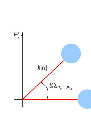
Figure 1: (Color online) Schematic diagram of the time evolution in phase space of the coherent state of the harmonic oscillator k𝑘k, corresponding to the product of number states j|mjjsubscriptproduct𝑗subscriptketsubscript𝑚𝑗𝑗\prod_{j}|m_{j}\rangle_{j}, where j=1,,A𝑗1𝐴j=1,\ldots,A. The coherent state with complex amplitude α𝛼\alpha is here depicted as a light blue circle in phase space (Xksubscript𝑋𝑘X_{k},Pksubscript𝑃𝑘P_{k}), where Xksubscript𝑋𝑘X_{k} and Pksubscript𝑃𝑘P_{k} represent the position and the momentum of the harmonic oscillator k𝑘k. After a time t𝑡t, the coherent state rotates about the origin with an angle tΩm1,,mA𝑡subscriptΩsubscript𝑚1subscript𝑚𝐴{t}\Omega_{m_{1},\ldots,m_{A}}.

We study the time evolution of the k𝑘k-th harmonic oscillator in phase space starting with a state j|mjj|αksubscriptproduct𝑗tensor-productsubscriptketsubscript𝑚𝑗𝑗subscriptket𝛼𝑘\prod_{j}|m_{j}\rangle_{j}\otimes|\alpha\rangle_{k}, where j|mjjsubscriptproduct𝑗subscriptketsubscript𝑚𝑗𝑗\prod_{j}|m_{j}\rangle_{j} is the product state of the number states of the harmonic oscillators, and |αksubscriptket𝛼𝑘|\alpha\rangle_{k} is the coherent state of the k𝑘k-th harmonic oscillator, for j=1,,A𝑗1𝐴j=1,\ldots,{A}, and k𝑘k is a number from A+1𝐴1A+1 to A+B𝐴𝐵A+B. By applying the time-evolution operator U(t)=exp(iHt)𝑈𝑡𝑖𝐻𝑡U(t)=\exp(-iHt) [H𝐻H is the Hamiltonian in Eq. (6)] to the initial state j|mjj|αksubscriptproduct𝑗subscriptketsubscript𝑚𝑗𝑗subscriptket𝛼𝑘\prod_{j}|m_{j}\rangle_{j}|\alpha\rangle_{k}, it becomes

U(t)j|mjj|αk𝑈𝑡subscriptproduct𝑗subscriptketsubscript𝑚𝑗𝑗subscriptket𝛼𝑘\displaystyle U(t)\prod_{j}|m_{j}\rangle_{j}|\alpha\rangle_{k} (9)
=\displaystyle= exp[i(jωjmj)t]j|mjj𝑖subscript𝑗subscript𝜔𝑗subscript𝑚𝑗𝑡subscriptproduct𝑗subscriptketsubscript𝑚𝑗𝑗\displaystyle\exp\bigg{[}-i\bigg{(}\sum_{j}\omega_{j}{m}_{j}\bigg{)}t\bigg{]}\prod_{j}|m_{j}\rangle_{j}
×exp{i[ωk+fk(m1,,mA)]akakt}|αk,absent𝑖delimited-[]subscript𝜔𝑘subscript𝑓𝑘subscript𝑚1subscript𝑚𝐴subscriptsuperscript𝑎𝑘subscript𝑎𝑘𝑡subscriptket𝛼𝑘\displaystyle\times\exp{\big{\{}-i[\omega_{k}+f_{k}(m_{1},\ldots,m_{A})]a^{\dagger}_{k}a_{k}{t}\big{\}}}|\alpha\rangle_{k},
=\displaystyle= exp[i(jωjmj)t]j|mjj|αm1,,mA(t)k,𝑖subscript𝑗subscript𝜔𝑗subscript𝑚𝑗𝑡subscriptproduct𝑗subscriptketsubscript𝑚𝑗𝑗subscriptketsubscript𝛼subscript𝑚1subscript𝑚𝐴𝑡𝑘\displaystyle\exp\bigg{[}-i\bigg{(}\sum_{j}\omega_{j}{m}_{j}\bigg{)}t\bigg{]}\prod_{j}|m_{j}\rangle_{j}|\alpha_{{m_{1},\ldots,m_{A}}}(t)\rangle_{k},

where αm1,,mA(t)subscript𝛼subscript𝑚1subscript𝑚𝐴𝑡\alpha_{m_{1},\ldots,m_{A}}(t) is a complex function, i.e.,

αm1,,mA(t)subscript𝛼subscript𝑚1subscript𝑚𝐴𝑡\displaystyle\alpha_{m_{1},\ldots,m_{A}}(t) =\displaystyle= exp[iΩm1,,mAt]α,𝑖subscriptΩsubscript𝑚1subscript𝑚𝐴𝑡𝛼\displaystyle\exp[-i\Omega_{m_{1},\ldots,m_{A}}t]\alpha, (10)

and Ωm1,,mAsubscriptΩsubscript𝑚1subscript𝑚𝐴\Omega_{m_{1},\ldots,m_{A}} is an effective rotation frequency of the coherent state in phase space

Ωm1,,mAsubscriptΩsubscript𝑚1subscript𝑚𝐴\displaystyle\Omega_{m_{1},\ldots,m_{A}} =\displaystyle= ωk+fk(m1,,mA).subscript𝜔𝑘subscript𝑓𝑘subscript𝑚1subscript𝑚𝐴\displaystyle\omega_{k}+f_{k}(m_{1},\ldots,m_{A}). (11)

In Eq. (9), we have used the relation Barnett ,

exp(iϑakak)|αk=|αexp(iϑ)k,𝑖italic-ϑsubscriptsuperscript𝑎𝑘subscript𝑎𝑘subscriptket𝛼𝑘subscriptket𝛼𝑖italic-ϑ𝑘\exp(-i\vartheta{a^{\dagger}_{k}{a}_{k}})|\alpha\rangle_{k}=|\alpha\exp(-i\vartheta)\rangle_{k}, (12)

where ϑitalic-ϑ\vartheta is a phase factor.

Note that the product state of the number states j|mjjsubscriptproduct𝑗subscriptketsubscript𝑚𝑗𝑗\prod_{j}|m_{j}\rangle_{j} is an invariant; namely it does not change with time. Nonlinear interactions, described by the Hamiltonian HIsubscript𝐻𝐼H_{I} in Eq. (5), cause the coherent state of oscillator k𝑘k to rotate about the origin with a frequency Ωm1,,mAsubscriptΩsubscript𝑚1subscript𝑚𝐴\Omega_{m_{1},\ldots,m_{A}} in phase space. From Eq. (11), the frequency Ωm1,,mAsubscriptΩsubscript𝑚1subscript𝑚𝐴\Omega_{m_{1},\ldots,m_{A}} depends on the number states j|mjjsubscriptproduct𝑗subscriptketsubscript𝑚𝑗𝑗\prod_{j}|m_{j}\rangle_{j} of the A𝐴A oscillators. A schematic diagram of the time evolution of the coherent state of the harmonic oscillator k𝑘k in phase space is shown in Fig. 1.

IV Factorization

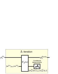
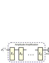
Extending our proposal in Ref. Ng , we now present an amplitude-amplification method to factor any positive integer N𝑁N. For example, let us consider three coupled harmonic oscillators for factorization by setting A=2𝐴2A=2 and B=1𝐵1B=1. Using this method, the probability of finding the factors’ state can reach nearly one after L𝐿L iterations. Simplified schematic diagrams of the factorization approach are shown in Figs. 2 and 3.
Refer to caption
Figure 2: (Color online) Factoring algorithm using three coupled harmonic oscillators. Initially, the state ρr(1)subscriptsuperscript𝜌1𝑟\rho^{(1)}_{r} of the harmonic oscillators 1 and 2, is prepared in a number-state basis. By repeatedly applying L𝐿L times the iterations Ilsubscript𝐼𝑙I_{l} (as shown in Fig. 3), the resulting state of the harmonic oscillators 1 and 2 becomes the state of the factors of N𝑁N. Finally, the factors of the number N𝑁N can be obtained by measuring the state of the oscillators 1 and 2.
Refer to caption
Figure 3: (Color online) The l𝑙l-th iteration, Ilsubscript𝐼𝑙I_{l}, in factorization. In each iteration, the third harmonic oscillator is prepared in a coherent state |α(l)3subscriptketsuperscript𝛼𝑙3|\alpha^{(l)}\rangle_{3} with a magnitude |α(l)|superscript𝛼𝑙|\alpha^{(l)}|. Then, a unitary operator Uf(tl)subscript𝑈𝑓subscript𝑡𝑙U_{f}(t_{l}) is applied. By performing a conditional measurement of the coherent state |αN(l)(tl)3subscriptketsubscriptsuperscript𝛼𝑙𝑁subscript𝑡𝑙3|\alpha^{(l)}_{N}(t_{l})\rangle_{3}, the reduced density matrix ρr(l+1)subscriptsuperscript𝜌𝑙1𝑟\rho^{(l+1)}_{r} can be obtained.

IV.1 Algorithm

Now we consider the total Hamiltonian Hfsubscript𝐻𝑓H_{f} of the system

Hf=j=13ωjajaj+ffactor(n1,n2)a3a3,subscript𝐻𝑓Planck-constant-over-2-pisubscriptsuperscript3𝑗1subscript𝜔𝑗subscriptsuperscript𝑎𝑗subscript𝑎𝑗Planck-constant-over-2-pisubscript𝑓factorsubscript𝑛1subscript𝑛2subscriptsuperscript𝑎3subscript𝑎3H_{f}=\hbar\sum^{3}_{j=1}{\omega_{j}}a^{\dagger}_{j}a_{j}+{\hbar}f_{\rm factor}(n_{1},n_{2})a^{\dagger}_{3}a_{3}, (13)

where the nonlinear-operator function ffactor(n1,n2)subscript𝑓factorsubscript𝑛1subscript𝑛2f_{\rm factor}(n_{1},n_{2}) for computing the product of any two trial factors is written as,

ffactor(n1,n2)=k=1Kgk(n1n2)k.subscript𝑓factorsubscript𝑛1subscript𝑛2subscriptsuperscript𝐾𝑘1subscript𝑔𝑘superscriptsubscript𝑛1subscript𝑛2𝑘f_{\rm factor}(n_{1},n_{2})=\sum^{K}_{k=1}g_{k}\,(n_{1}n_{2})^{k}. (14)

Here the parameters gksubscript𝑔𝑘g_{k} are the coupling strengths of the nonlinear interactions (n1n2)ka3a3superscriptsubscript𝑛1subscript𝑛2𝑘subscriptsuperscript𝑎3subscript𝑎3(n_{1}n_{2})^{k}a^{\dagger}_{3}a_{3}, for k=1,,K𝑘1𝐾k=1,\ldots,K. This operator function ffactorsubscript𝑓factorf_{\rm factor} will output an eigenvalue which is a power series of the product n×m𝑛𝑚n\times{m}, for the product state |n,m=|n1|m2ket𝑛𝑚subscriptket𝑛1subscriptket𝑚2|n,m\rangle=|n\rangle_{1}\;|m\rangle_{2}.

The total state of the first two harmonic oscillators, in the number state basis, is initially prepared, i.e.,

ρr(1)subscriptsuperscript𝜌1𝑟\displaystyle\rho^{(1)}_{r} =\displaystyle= n,n,m,mpnmnm|n,mn,m|,subscript𝑛superscript𝑛𝑚superscript𝑚subscriptsuperscript𝑝superscript𝑛superscript𝑚𝑛𝑚ket𝑛𝑚brasuperscript𝑛superscript𝑚\displaystyle\sum_{n,n^{\prime},m,m^{\prime}}p^{n^{\prime}m^{\prime}}_{nm}|n,m\rangle\langle{n^{\prime}},{m^{\prime}}|, (15)

where the pnmnmsubscriptsuperscript𝑝superscript𝑛superscript𝑚𝑛𝑚p^{n^{\prime}m^{\prime}}_{nm} are the probabilities of the states of the first and second oscillators, while n,n,m,m=2,,N/2formulae-sequence𝑛superscript𝑛𝑚superscript𝑚2𝑁2n,n^{\prime},m,m^{\prime}=2,\ldots,{N/2}. The states of the harmonic oscillators 1 and 2 can be prepared in arbitrary states, including pure states or mixed states Ng . The states of oscillators 1 and 2 encode all trial factors of the number N𝑁N. Each number state |njsubscriptket𝑛𝑗|n\rangle_{j} represents each trial factor n𝑛n, for j=1,2𝑗12j=1,2.

IV.1.1 First iteration: I1subscript𝐼1I_{1}

In the first iteration, the state of the third harmonic oscillator is prepared in a coherent state |α(1)3subscriptketsuperscript𝛼13|\alpha^{(1)}\rangle_{3}. By applying the time-evolution operator Uf(t1)=exp(iHft1)subscript𝑈𝑓subscript𝑡1𝑖subscript𝐻𝑓subscript𝑡1U_{f}(t_{1})=\exp(-iH_{f}t_{1}) to the initial state ρ(1)(0)=ρr(1)|α(1)33α(1)|\rho^{(1)}(0)=\rho^{(1)}_{r}\otimes|\alpha^{(1)}\rangle_{3}\;{}_{3}\langle\alpha^{(1)}|, it becomes

ρ(1)(t1)superscript𝜌1subscript𝑡1\displaystyle\rho^{(1)}(t_{1}) =\displaystyle= Uf(t1)ρr(1)|α(1)33α(1)|Uf(t1),\displaystyle U_{f}(t_{1})\rho^{(1)}_{r}\otimes|\alpha^{(1)}\rangle_{3}\;{}_{3}\langle\alpha^{(1)}|U^{{\dagger}}_{f}(t_{1}), (16)
=\displaystyle= n,m,n,mp~nmnm|n,m|αnm(1)(t1)33αnm(1)(t1)|n,m|\displaystyle\sum_{n,m,n^{\prime},m^{\prime}}\tilde{p}^{n^{\prime}m^{\prime}}_{nm}|n,m\rangle|\alpha^{(1)}_{nm}(t_{1})\rangle_{3}\;{}_{3}\langle\alpha^{(1)}_{n^{\prime}m^{\prime}}(t_{1})|\langle{n^{\prime},m^{\prime}}| (17)

where

p~nmnm(t1)=exp{i[(nn)ω1+(mm)ω2]t1}pnmnm.subscriptsuperscript~𝑝superscript𝑛superscript𝑚𝑛𝑚subscript𝑡1𝑖delimited-[]superscript𝑛𝑛subscript𝜔1superscript𝑚𝑚subscript𝜔2subscript𝑡1subscriptsuperscript𝑝superscript𝑛superscript𝑚𝑛𝑚\tilde{p}^{n^{\prime}m^{\prime}}_{nm}(t_{1})=\exp\{i[(n^{\prime}-n)\omega_{1}+(m^{\prime}-m)\omega_{2}]t_{1}\}p^{n^{\prime}m^{\prime}}_{nm}. (18)

Here αnm(l)(t)subscriptsuperscript𝛼𝑙𝑛𝑚𝑡\alpha^{(l)}_{nm}(t), for l=1𝑙1l=1, in Eq. (17) is a complex function,

αnm(l)(t)subscriptsuperscript𝛼𝑙𝑛𝑚𝑡\displaystyle\alpha^{(l)}_{nm}(t) =\displaystyle= exp(iΩnmt)α(l),𝑖subscriptΩ𝑛𝑚𝑡superscript𝛼𝑙\displaystyle\exp(-i\Omega_{nm}t)\alpha^{(l)}, (19)

and ΩnmsubscriptΩ𝑛𝑚\Omega_{nm} is an effective rotation frequency of the coherent state in phase space

ΩnmsubscriptΩ𝑛𝑚\displaystyle\Omega_{nm} =\displaystyle= ω3+k=1Kgk(nm)k.subscript𝜔3subscriptsuperscript𝐾𝑘1subscript𝑔𝑘superscript𝑛𝑚𝑘\displaystyle\omega_{3}+\sum^{K}_{k=1}g_{k}(nm)^{k}. (20)

Note that the product of the two factors of r𝑟r and s𝑠s is equal to N𝑁N: r×s=N𝑟𝑠𝑁r\times{s}=N. The rotation frequency ΩNsubscriptΩ𝑁\Omega_{N} of the coherent state is

ΩNsubscriptΩ𝑁\displaystyle\Omega_{N} =\displaystyle= ω3+k=1KgkNk.subscript𝜔3subscriptsuperscript𝐾𝑘1subscript𝑔𝑘superscript𝑁𝑘\displaystyle\omega_{3}+\sum^{K}_{k=1}g_{k}N^{k}. (21)

If the product of any two numbers is not equal to N𝑁N, then the frequencies ΩnmsubscriptΩ𝑛𝑚\Omega_{nm} are different to the frequency ΩNsubscriptΩ𝑁\Omega_{N}. Thus, the state of the harmonic oscillator 3 can act as a “marker” for the states of factors and non-factors Ng .

Now we define a measurement operator lsubscript𝑙\mathcal{M}_{l} which can be written as Wiseman

lρ(l)(tl)subscript𝑙superscript𝜌𝑙subscript𝑡𝑙\displaystyle\mathcal{M}_{l}\>\rho^{(l)}(t_{l})\, =\displaystyle= 𝒥(El)ρ(l)(tl)=lElρ(l)(tl)El,𝒥subscript𝐸𝑙superscript𝜌𝑙subscript𝑡𝑙subscript𝑙subscript𝐸𝑙superscript𝜌𝑙subscript𝑡𝑙subscriptsuperscript𝐸𝑙\displaystyle\,\mathcal{J}(E_{l})\rho^{(l)}(t_{l})\,=\,\sum_{l}E_{l}\>{\rho^{(l)}}(t_{l})\>E^{{\dagger}}_{l}, (22)
Elsubscript𝐸𝑙\displaystyle E_{l}\, =\displaystyle= |αN(l)(tl)33αN(l)(tl)|,\displaystyle\,|\alpha^{(l)}_{N}(t_{l})\rangle_{3}\;{}_{3}{\langle}\alpha^{(l)}_{N}(t_{l})|, (23)

where αN(l)(tl)=α(l)exp(iΩNtl)subscriptsuperscript𝛼𝑙𝑁subscript𝑡𝑙superscript𝛼𝑙𝑖subscriptΩ𝑁subscript𝑡𝑙\alpha^{(l)}_{N}(t_{l})=\alpha^{(l)}\exp(-i\Omega_{N}t_{l}) and l𝑙l is the number of iterations. A conditional measurement 1subscript1\mathcal{M}_{1} is performed on the third oscillator at the time t1subscript𝑡1t_{1}. The probability of obtaining this coherent state |αN(1)(t1)3subscriptketsuperscriptsubscript𝛼𝑁1subscript𝑡13|\alpha_{N}^{(1)}(t_{1})\rangle_{3} becomes

Pr(E1)Prsubscript𝐸1\displaystyle{\rm Pr}(E_{1}) =\displaystyle= Tr[1ρ(1)(t1)],Trdelimited-[]subscript1superscript𝜌1subscript𝑡1\displaystyle{\rm Tr}[\mathcal{M}_{1}\rho^{(1)}(t_{1})], (24)
=\displaystyle= n,mpnmnm|ϵnm(1)|2,subscript𝑛𝑚subscriptsuperscript𝑝𝑛𝑚𝑛𝑚superscriptsubscriptsuperscriptitalic-ϵ1𝑛𝑚2\displaystyle\sum_{n,m}{p}^{nm}_{nm}\;|{\epsilon}^{(1)}_{nm}|^{2}, (25)

where the coefficient ϵnm(l)=αN(l)(tl)|αnm(l)(tl)33\epsilon^{(l)}_{nm}={}_{3}\langle{\alpha}^{(l)}_{N}(t_{l})|\alpha^{(l)}_{nm}(t_{l})\rangle_{3}, for l=1𝑙1l=1, and

ϵnm(l)subscriptsuperscriptitalic-ϵ𝑙𝑛𝑚\displaystyle\epsilon^{(l)}_{nm} =\displaystyle= exp{|α(l)|2[1exp(iΩNtliΩnmtl)]},forl1,superscriptsuperscript𝛼𝑙2delimited-[]1𝑖subscriptΩ𝑁subscript𝑡𝑙𝑖subscriptΩ𝑛𝑚subscript𝑡𝑙for𝑙1\displaystyle\exp\{-|\alpha^{(l)}|^{2}[1-\exp(i\Omega_{N}{t}_{l}-i\Omega_{nm}t_{l})]\},~{}~{}~{}~{}{\rm for}~{}~{}l\geqslant{1}, (26)

is the overlap between the two coherent states |αN(l)(tl)3subscriptketsubscriptsuperscript𝛼𝑙𝑁subscript𝑡𝑙3|\alpha^{(l)}_{N}(t_{l})\rangle_{3} and |αnm(l)(tl)3subscriptketsubscriptsuperscript𝛼𝑙𝑛𝑚subscript𝑡𝑙3|\alpha^{(l)}_{nm}(t_{l})\rangle_{3}, respectively. Note that the value of the probability Pr(E1)Prsubscript𝐸1{\rm Pr}(E_{1}) can be adjusted by appropriately choosing the evolution time and the magnitude |α(1)|superscript𝛼1|\alpha^{(1)}|. In practice, this probability Pr(E1)Prsubscript𝐸1{\rm Pr}(E_{1}) cannot be adjusted to be extremely small.

Recall that a state is conditioned when this state is conditional on the measurement of a certain state Wiseman . After the measurement of |αN(1)(t1)3subscriptketsubscriptsuperscript𝛼1𝑁subscript𝑡13|\alpha^{(1)}_{N}(t_{1})\rangle_{3}, the density matrix of the conditioned state can be written as Wiseman :

ρc(1)subscriptsuperscript𝜌1𝑐\displaystyle\rho^{(1)}_{c} =\displaystyle= 1ρ(1)(t1)Tr[1ρ(1)(t1)],subscript1superscript𝜌1subscript𝑡1Trdelimited-[]subscript1superscript𝜌1subscript𝑡1\displaystyle\frac{\mathcal{M}_{1}\rho^{(1)}(t_{1})}{{\rm Tr}[\mathcal{M}_{1}\rho^{(1)}(t_{1})]}, (27)
=\displaystyle= 1C1n,m,n,mp~nmnm(t1)ϵnm(1)ϵnm(1)|n,mn,m||αN(1)(t1)33αN(1)(t1)|,\displaystyle\frac{1}{C_{1}}\sum_{n,m,n^{\prime},m^{\prime}}\!\!\tilde{p}^{n^{\prime}m^{\prime}}_{nm}\!(t_{1})\;{\epsilon}^{(1)}_{nm}\;{\epsilon}^{(1)*}_{n^{\prime}m^{\prime}}|n,m\rangle\langle{n^{\prime},m^{\prime}}|\otimes|\alpha^{(1)}_{N}(t_{1})\rangle_{3}\;{}_{3}{\langle}\alpha^{(1)}_{N}(t_{1})|, (28)

where C1subscript𝐶1C_{1} is a normalization constant

C1subscript𝐶1\displaystyle C_{1} =\displaystyle= n,mpnmnm|ϵnm(1)|2.subscript𝑛𝑚subscriptsuperscript𝑝𝑛𝑚𝑛𝑚superscriptsubscriptsuperscriptitalic-ϵ1𝑛𝑚2\displaystyle\sum_{n,m}{p}^{nm}_{nm}\;|{\epsilon}^{(1)}_{nm}|^{2}. (29)

Note that the trace of this density matrix Tr[ρ(1)]Trdelimited-[]superscript𝜌1{\rm Tr}[\rho^{(1)}] is equal to one. After the first iteration, the probability of finding the factors of the number N𝑁N is increased by a factor C11subscriptsuperscript𝐶11C^{-1}_{1}, which is the inverse of the probability Pr(E1)Prsubscript𝐸1{\rm Pr}(E_{1}) as seen from Eqs. (25) and (28). The probability amplification [see also Eqs. (53) and (54)] is thus inversely proportional to the probability of obtaining the coherent state Pr(E1)Prsubscript𝐸1{\rm Pr}(E_{1}).

IV.1.2 Second iteration: I2subscript𝐼2I_{2}

After the first iteration, we now obtain the reduced density matrix ρr(2)subscriptsuperscript𝜌2𝑟\rho^{(2)}_{r} of the first two harmonic oscillators as

ρr(2)subscriptsuperscript𝜌2𝑟\displaystyle\rho^{(2)}_{r} =\displaystyle= 1C1n,m,n,mp~nmnm(t1)ϵnm(1)ϵnm(1)|n,mn,m|.1subscript𝐶1subscript𝑛𝑚superscript𝑛superscript𝑚subscriptsuperscript~𝑝superscript𝑛superscript𝑚𝑛𝑚subscript𝑡1subscriptsuperscriptitalic-ϵ1𝑛𝑚subscriptsuperscriptitalic-ϵ1superscript𝑛superscript𝑚ket𝑛𝑚brasuperscript𝑛superscript𝑚\displaystyle\frac{1}{C_{1}}\sum_{n,m,n^{\prime},m^{\prime}}\tilde{p}^{n^{\prime}m^{\prime}}_{nm}(t_{1}){\epsilon}^{(1)}_{nm}{\epsilon}^{(1)*}_{n^{\prime}m^{\prime}}|n,m\rangle\langle{n^{\prime},m^{\prime}}|. (30)

We consider the state ρr(2)subscriptsuperscript𝜌2𝑟\rho^{(2)}_{r} in Eq. (30) of the oscillators 1 and 2 as an input state for the second iteration. The coherent state of the third harmonic oscillator is prepared in a coherent state |α(2)3subscriptketsuperscript𝛼23|\alpha^{(2)}\rangle_{3}, with a magnitude |α(2)|superscript𝛼2|\alpha^{(2)}|. The nonlinear interactions between the three harmonic oscillators are then turned on for a time t2subscript𝑡2t_{2}. The state evolves as

ρ(2)(t2)superscript𝜌2subscript𝑡2\displaystyle\rho^{(2)}(t_{2}) =\displaystyle= 1C1n,m,n,mp~nmnm(t~2)ϵnm(1)ϵnm(1)|n,m|αnm(2)(t2)33αnm(2)(t2)|n,m|,\displaystyle\frac{1}{C_{1}}\!\sum_{n,m,n^{\prime},m^{\prime}}\!\!\tilde{p}^{n^{\prime}m^{\prime}}_{nm}\!(\tilde{t}_{2})\;{\epsilon}^{(1)}_{nm}\;{\epsilon}^{(1)*}_{n^{\prime}m^{\prime}}|n,m\rangle|\alpha^{(2)}_{nm}(t_{2})\rangle_{3}\;{}_{3}{\langle}\alpha^{(2)}_{n^{\prime}m^{\prime}}(t_{2})|\langle{n^{\prime},m^{\prime}}|, (31)

where t~2=t1+t2subscript~𝑡2subscript𝑡1subscript𝑡2\tilde{t}_{2}=t_{1}+t_{2}.

Next, a conditional measurement 2subscript2\mathcal{M}_{2} is applied to the system at the time t2subscript𝑡2t_{2}. The probability of obtaining the coherent state |αN(2)(t2)3subscriptketsubscriptsuperscript𝛼2𝑁subscript𝑡23|\alpha^{(2)}_{N}(t_{2})\rangle_{3} becomes

Pr(E2)Prsubscript𝐸2\displaystyle{\rm Pr}(E_{2}) =\displaystyle= Tr[2ρ(2)(t2)],Trdelimited-[]subscript2superscript𝜌2subscript𝑡2\displaystyle{\rm Tr}[\mathcal{M}_{2}\rho^{(2)}(t_{2})], (32)
=\displaystyle= 1C1n,mpnmnm|ϵnm(1)|2|ϵnm(2)|2.1subscript𝐶1subscript𝑛𝑚subscriptsuperscript𝑝𝑛𝑚𝑛𝑚superscriptsubscriptsuperscriptitalic-ϵ1𝑛𝑚2superscriptsubscriptsuperscriptitalic-ϵ2𝑛𝑚2\displaystyle\frac{1}{C_{1}}\sum_{n,m}{p}^{nm}_{nm}\;|{\epsilon}^{(1)}_{nm}|^{2}\;|{\epsilon}^{(2)}_{nm}|^{2}. (33)

The conditioned state can be written as

ρc(2)subscriptsuperscript𝜌2𝑐\displaystyle\rho^{(2)}_{c} =\displaystyle= 2ρ(2)(t2)Tr[2ρ(2)(t2)],subscript2superscript𝜌2subscript𝑡2Trdelimited-[]subscript2superscript𝜌2subscript𝑡2\displaystyle\frac{\mathcal{M}_{2}\rho^{(2)}(t_{2})}{{\rm Tr}[{\mathcal{M}_{2}\rho^{(2)}(t_{2})}]}, (34)
=\displaystyle= 1C2n,m,n,mp~nmnm(t~2)ϵnm(1)ϵnm(1)ϵnm(2)ϵnm(2)|n,mn,m||αN(2)(t2)33αN(2)(t2)|,\displaystyle\frac{1}{C_{2}}\sum_{n,m,n^{\prime},m^{\prime}}\tilde{p}^{n^{\prime}m^{\prime}}_{nm}(\tilde{t}_{2}){\epsilon}^{(1)}_{nm}{\epsilon}^{(1)*}_{n^{\prime}m^{\prime}}{\epsilon}^{(2)}_{nm}{\epsilon}^{(2)*}_{n^{\prime}m^{\prime}}|n,m\rangle\langle{n^{\prime},m^{\prime}}|\otimes|\alpha^{(2)}_{N}(t_{2})\rangle_{3}\;{}_{3}{\langle}\alpha^{(2)}_{N}(t_{2})|, (35)

where C2subscript𝐶2C_{2} is the normalization constant,

C2=n,mpnmnm|ϵnm(1)|2|ϵnm(2)|2.subscript𝐶2subscript𝑛𝑚subscriptsuperscript𝑝𝑛𝑚𝑛𝑚superscriptsubscriptsuperscriptitalic-ϵ1𝑛𝑚2superscriptsubscriptsuperscriptitalic-ϵ2𝑛𝑚2C_{2}=\sum_{n,m}{p}^{nm}_{nm}|{\epsilon}^{(1)}_{nm}|^{2}|{\epsilon}^{(2)}_{nm}|^{2}. (36)

The probability of finding the factors is enhanced by a factor C21subscriptsuperscript𝐶12C^{-1}_{2} after the second iteration.

The coefficients |ϵnm(2)|subscriptsuperscriptitalic-ϵ2𝑛𝑚|\epsilon^{(2)}_{nm}| is less than one for any product n×mN𝑛𝑚𝑁n\times{m}\neq{N}. From Eqs. (29) and (36), it can be seen that C2<C1subscript𝐶2subscript𝐶1C_{2}<{C_{1}}. Therefore, the probability of finding the factors is now higher after one additional iteration.

IV.1.3 L𝐿L-th iteration: ILsubscript𝐼𝐿I_{L}

Similarly, we now iterate the procedure (L1)𝐿1(L-1) times. After (L1)𝐿1(L-1) iterations, the reduced density matrix of the oscillators 1 and 2 can be written as

ρr(L)subscriptsuperscript𝜌𝐿𝑟\displaystyle\rho^{(L)}_{r} =\displaystyle= 1CL1n,m,n,mp~nmnm(t~L1)l=1L1ϵnm(l)ϵnm(l)|n,mn,m|,1subscript𝐶𝐿1subscript𝑛𝑚superscript𝑛superscript𝑚subscriptsuperscript~𝑝superscript𝑛superscript𝑚𝑛𝑚subscript~𝑡𝐿1subscriptsuperscriptproduct𝐿1𝑙1subscriptsuperscriptitalic-ϵ𝑙𝑛𝑚subscriptsuperscriptitalic-ϵ𝑙superscript𝑛superscript𝑚ket𝑛𝑚brasuperscript𝑛superscript𝑚\displaystyle\frac{1}{C_{L-1}}\!\!\sum_{n,m,n^{\prime},m^{\prime}}\!\!\tilde{p}^{n^{\prime}m^{\prime}}_{nm}\!(\tilde{t}_{L-1})\prod^{L-1}_{l=1}{\epsilon}^{(l)}_{nm}\;{\epsilon}^{(l)*}_{n^{\prime}m^{\prime}}|n,m\rangle\langle{n^{\prime},m^{\prime}}|, (37)

where

CL1subscript𝐶𝐿1\displaystyle C_{L-1} =\displaystyle= n,mpnmnml=1L1|ϵnm(l)|2,subscript𝑛𝑚subscriptsuperscript𝑝𝑛𝑚𝑛𝑚subscriptsuperscriptproduct𝐿1𝑙1superscriptsubscriptsuperscriptitalic-ϵ𝑙𝑛𝑚2\displaystyle\sum_{n,m}{p}^{nm}_{nm}\prod^{L-1}_{l=1}|{\epsilon}^{(l)}_{nm}|^{2}, (38)
t~L1subscript~𝑡𝐿1\displaystyle\tilde{t}_{L-1} =\displaystyle= l=1L1tl.subscriptsuperscript𝐿1𝑙1subscript𝑡𝑙\displaystyle\sum^{L-1}_{l=1}t_{l}. (39)

The state of the third harmonic oscillator is now prepared in a coherent state |α(L)3subscriptketsuperscript𝛼𝐿3|\alpha^{(L)}\rangle_{3}, with a magnitude |α(L)|superscript𝛼𝐿|\alpha^{(L)}|. Let the three coupled harmonic oscillators evolve for a time tLsubscript𝑡𝐿t_{L}. This gives

ρ(L)(tL)superscript𝜌𝐿subscript𝑡𝐿\displaystyle\rho^{(L)}(t_{L}) =\displaystyle= 1CL1n,m,n,mp~nmnm(t~L)l=1L1ϵnm(l)ϵnm(l)|n,m|αnm(L)(tL)33αnm(L)(tL)|n,m|.\displaystyle\frac{1}{C_{L-1}}\!\!\sum_{n,m,n^{\prime},m^{\prime}}\!\!\tilde{p}^{n^{\prime}m^{\prime}}_{nm}\!(\tilde{t}_{L})\prod^{L-1}_{l=1}{\epsilon}^{(l)}_{nm}\;{\epsilon}^{(l)*}_{n^{\prime}m^{\prime}}|n,m\rangle|\alpha^{(L)}_{nm}(t_{L})\rangle_{3}\;{}_{3}{\langle}\alpha^{(L)}_{n^{\prime}m^{\prime}}(t_{L})|\langle{n^{\prime},m^{\prime}}|. (40)

By performing a conditional measurement |αN(L)(tL)3subscriptketsubscriptsuperscript𝛼𝐿𝑁subscript𝑡𝐿3|\alpha^{(L)}_{N}(t_{L})\rangle_{3}, the state becomes

ρc(L)subscriptsuperscript𝜌𝐿𝑐\displaystyle\rho^{(L)}_{c} =\displaystyle= Lρ(L)(tL)Tr[Lρ(L)(tL)],subscript𝐿superscript𝜌𝐿subscript𝑡𝐿Trdelimited-[]subscript𝐿superscript𝜌𝐿subscript𝑡𝐿\displaystyle\frac{\mathcal{M}_{L}\rho^{(L)}(t_{L})}{{\rm Tr}[\mathcal{M}_{L}\rho^{(L)}(t_{L})]}, (41)
=\displaystyle= 1CLn,m,n,mp~nmnm(t~L)l=1Lϵnm(l)ϵnm(l)|n,mn,m||αN(L)(tL)33αN(L)(tL)|.\displaystyle\frac{1}{C_{L}}\sum_{n,m,n^{\prime},m^{\prime}}\tilde{p}^{n^{\prime}m^{\prime}}_{nm}(\tilde{t}_{L})\prod^{L}_{l=1}{\epsilon}^{(l)}_{nm}{\epsilon}^{(l)*}_{n^{\prime}m^{\prime}}|n,m\rangle\langle{n^{\prime},m^{\prime}}|\otimes|\alpha^{(L)}_{N}(t_{L})\rangle_{3}\;{}_{3}\langle\alpha^{(L)}_{N}(t_{L})|. (42)

After the L𝐿L-th step, the probability of finding the factors is increased by a factor CL1subscriptsuperscript𝐶1𝐿C^{-1}_{L}. From Eq. (38), the probability of obtaining the coherent state |αN(L)(tL)3subscriptketsubscriptsuperscript𝛼𝐿𝑁subscript𝑡𝐿3|\alpha^{(L)}_{N}(t_{L})\rangle_{3} can be written as

Pr(EL)Prsubscript𝐸𝐿\displaystyle{\rm Pr}(E_{L}) =\displaystyle= 1CL1n,mpnmnml=1L|ϵnm(l)|2,1subscript𝐶𝐿1subscript𝑛𝑚subscriptsuperscript𝑝𝑛𝑚𝑛𝑚subscriptsuperscriptproduct𝐿𝑙1superscriptsubscriptsuperscriptitalic-ϵ𝑙𝑛𝑚2\displaystyle\frac{1}{C_{L-1}}\sum_{n,m}{p}^{nm}_{nm}\prod^{L}_{l=1}|{\epsilon}^{(l)}_{nm}|^{2}, (43)
=\displaystyle= CLCL1.subscript𝐶𝐿subscript𝐶𝐿1\displaystyle\frac{C_{L}}{C_{L-1}}. (44)

The entire iterative procedure is now completed. The convergence and performance of this method will be discussed in the following subsections.

IV.2 Convergence

We now study the convergence of this iterative method. We first consider the magnitude of the coherent state |α(l)|superscript𝛼𝑙|\alpha^{(l)}| for each iteration as

|α(1)||α(2)||α(l)||α(L)|.superscript𝛼1superscript𝛼2superscript𝛼𝑙superscript𝛼𝐿|\alpha^{(1)}|\leqslant|\alpha^{(2)}|\leqslant\ldots\leqslant|\alpha^{(l)}|\leqslant\ldots\leqslant|\alpha^{(L)}|. (45)

Thus, we have

1>|ϵnm(1)|2|ϵnm(2)|2|ϵnm(l)|2|ϵnm(L)|2.1superscriptsubscriptsuperscriptitalic-ϵ1𝑛𝑚2superscriptsubscriptsuperscriptitalic-ϵ2𝑛𝑚2superscriptsubscriptsuperscriptitalic-ϵ𝑙𝑛𝑚2superscriptsubscriptsuperscriptitalic-ϵ𝐿𝑛𝑚21>|{\epsilon}^{(1)}_{nm}|^{2}\geqslant|{\epsilon}^{(2)}_{nm}|^{2}\geqslant\ldots\geqslant|{\epsilon}^{(l)}_{nm}|^{2}\geqslant\ldots\geqslant|{\epsilon}^{(L)}_{nm}|^{2}. (46)

For any product of n𝑛n and m𝑚m being not equal to N𝑁N, the coefficient |ϵnm(l)|2superscriptsubscriptsuperscriptitalic-ϵ𝑙𝑛𝑚2|{\epsilon}^{(l)}_{nm}|^{2} is less than one and decreasing for higher l𝑙l, and the evolution time tlsubscript𝑡𝑙t_{l} is non-zero and appropriately chosen. When the number of iterations L𝐿L tends to infinity, the product of the coefficients |ϵnm(l)|2superscriptsubscriptsuperscriptitalic-ϵ𝑙𝑛𝑚2|{\epsilon}^{(l)}_{nm}|^{2} tends to zero,

limLl=1L|ϵnm(l)|20.subscript𝐿subscriptsuperscriptproduct𝐿𝑙1superscriptsubscriptsuperscriptitalic-ϵ𝑙𝑛𝑚20\lim_{L\rightarrow\infty}\prod^{L}_{l=1}|{\epsilon}^{(l)}_{nm}|^{2}\rightarrow{0}. (47)

The coefficients |ϵrs(l)|2superscriptsubscriptsuperscriptitalic-ϵ𝑙𝑟𝑠2|{\epsilon}^{(l)}_{rs}|^{2} are equal to one for any product of two factors r𝑟r and s𝑠s being equal to N𝑁N, i.e., when r×s=N𝑟𝑠𝑁r\times{s}=N.

Now we consider the probability of finding a pair of factors, r𝑟r and s𝑠s, after the l𝑙l-th iteration, which is

Prl(|r,s)subscriptPr𝑙ket𝑟𝑠\displaystyle{\rm Pr}_{l}\big{(}|{r},{s}\rangle\big{)} =\displaystyle= pr,sr,sCl.subscriptsuperscript𝑝𝑟𝑠𝑟𝑠subscript𝐶𝑙\displaystyle\frac{p^{{r},{s}}_{{r},{s}}}{C_{l}}. (48)

Since the coefficient |ϵnm(l)|2superscriptsubscriptsuperscriptitalic-ϵ𝑙𝑛𝑚2|\epsilon^{(l)}_{nm}|^{2} is less than one, the normalization constant Clsubscript𝐶𝑙C_{l} in Eq. (38) is decreasing, i.e., Cl<Cl1subscript𝐶𝑙subscript𝐶𝑙1C_{l}\;{<}\;C_{l-1}. Therefore, the probability of finding a pair of factors increases after an additional iteration. This shows that this iterative method is convergent.

From Eqs. (38) and (47), it is very easy to show that

limLCLsubscript𝐿subscript𝐶𝐿\displaystyle\lim_{L\rightarrow\infty}C_{L} =\displaystyle= limLn,mpnmnml=1L|ϵnm(l)|2subscript𝐿subscript𝑛𝑚subscriptsuperscript𝑝𝑛𝑚𝑛𝑚subscriptsuperscriptproduct𝐿𝑙1superscriptsubscriptsuperscriptitalic-ϵ𝑙𝑛𝑚2\displaystyle\lim_{L\rightarrow\infty}\sum_{n,m}p^{nm}_{nm}\prod^{L}_{l=1}|\epsilon^{(l)}_{nm}|^{2} (49)
=\displaystyle= r,sprsrs.subscript𝑟𝑠subscriptsuperscript𝑝𝑟𝑠𝑟𝑠\displaystyle\sum_{r,s}{p}^{rs}_{rs}. (50)

In the limit of large number of iterations L𝐿L, we can obtain the state ρfsubscript𝜌𝑓\rho_{f} of the factors

limLρr(L)subscript𝐿subscriptsuperscript𝜌𝐿𝑟\displaystyle\lim_{L\rightarrow\infty}\rho^{(L)}_{r} \displaystyle\rightarrow ρf,subscript𝜌𝑓\displaystyle\rho_{f}, (51)

where

ρf=1Cfr,s,r,sprsrs|r,sr,s|,subscript𝜌𝑓1subscriptsuperscript𝐶𝑓subscript𝑟𝑠superscript𝑟superscript𝑠subscriptsuperscript𝑝superscript𝑟superscript𝑠𝑟𝑠ket𝑟𝑠brasuperscript𝑟superscript𝑠\displaystyle\rho_{f}=\frac{1}{C^{*}_{f}}\sum_{r,s,r^{\prime},s^{\prime}}{p}^{r^{\prime}s^{\prime}}_{rs}|r,s\rangle\langle{r^{\prime},s^{\prime}}|, (52)

and Cf=r,sprsrssubscriptsuperscript𝐶𝑓subscript𝑟𝑠subscriptsuperscript𝑝𝑟𝑠𝑟𝑠C^{*}_{f}=\sum_{r,s}{p}^{rs}_{rs}, with r,s,r,s𝑟𝑠superscript𝑟superscript𝑠r,s,r^{\prime},s^{\prime} are factors of N𝑁N (r×s=r×s=N𝑟𝑠superscript𝑟superscript𝑠𝑁r{\times}s=r^{\prime}{\times}s^{\prime}=N). This shows that the state of the factors can be achieved by employing this iterative method, if a sufficiently large number of iterations is used.

IV.3 Performance

We can now estimate the number L𝐿L of the iterations required to achieve a probability of order of one for factoring N𝑁N. We investigate the amplification ratio λlsubscript𝜆𝑙\lambda_{l} of the two probabilities of finding the factors Prl1(|r,s)subscriptPr𝑙1ket𝑟𝑠{\rm Pr}_{l-1}\big{(}|{r},{s}\rangle\big{)} and Prl(|r,s)subscriptPr𝑙ket𝑟𝑠{\rm Pr}_{l}\big{(}|{r},{s}\rangle\big{)} after the (l1)𝑙1(l-1)-th and the l𝑙l-th iterations. From Eq. (48), we have

λlsubscript𝜆𝑙\displaystyle\lambda_{l} =\displaystyle= Prl(|r,s)Prl1(|r,s),subscriptPr𝑙ket𝑟𝑠subscriptPr𝑙1ket𝑟𝑠\displaystyle\frac{{\rm Pr}_{l}\big{(}|{r},{s}\rangle\big{)}}{{\rm Pr}_{l-1}\big{(}|{r},{s}\rangle\big{)}}, (53)
=\displaystyle= Cl1Cl.subscript𝐶𝑙1subscript𝐶𝑙\displaystyle\frac{C_{l-1}}{C_{l}}. (54)

Note that this ratio λlsubscript𝜆𝑙\lambda_{l} is just the reciprocal Pr1(El)superscriptPr1subscript𝐸𝑙{\rm Pr}^{-1}(E_{l}) in Eq. (44) of the probability of obtaining the coherent state. Practically, this probability Pr(El)Prsubscript𝐸𝑙{\rm Pr}(E_{l}) cannot be too small. For example, let the amplification ratio λlsubscript𝜆𝑙\lambda_{l} be roughly equal to λO(101)similar-to𝜆𝑂superscript101{\lambda}{~{}\sim~{}}O(10^{-1}) for each iteration, and let the probability of the factors’ state Pr0(|r,s)subscriptPr0ket𝑟𝑠{\rm Pr}_{0}\big{(}|r,s\rangle\big{)} before the iterations be of order O(Nz)𝑂superscript𝑁𝑧{O}(N^{-z}), where z𝑧z is a positive number. After L𝐿L iterations, the probability of finding the states of the factors can be increased by a factor λLsuperscript𝜆𝐿\lambda^{L}. Here we require

O(λL)O(Nz).similar-to𝑂superscript𝜆𝐿𝑂superscript𝑁𝑧\displaystyle{O}(\lambda^{L})\sim{O}(N^{z}). (55)

Therefore, we obtain that the number L𝐿L of necessary iterations is of order of O(log2N)𝑂subscript2𝑁{O}({\log_{2}{N}}). In the limit of large L𝐿L, the probabilities Pr(El)Prsubscript𝐸𝑙{\rm Pr}(E_{l}) in Eq. (44) tend to one because CLsubscript𝐶𝐿C_{L} approaches the sum of probabilities of the factors’ states in Eq. (50). The probability of finding the factors will be slowly increased after the number LO(log2N)similar-to𝐿𝑂subscript2𝑁L\sim{O}(\log_{2}{N}) of iterations is reached.

IV.4 Example: Initial pure states

In this section, we study how to factorize an integer N𝑁N with an initial pure state using this factoring algorithm. We consider the initial state of the first two harmonic oscillators as the superposition of number states, i.e.,

|Ψ(0)ketΨ0\displaystyle|\Psi(0)\rangle =\displaystyle= (1D1n=3N|n1)(1D2m=N+1N/3|m2),1subscript𝐷1subscriptsuperscript𝑁𝑛3subscriptket𝑛11subscript𝐷2subscriptsuperscript𝑁3𝑚𝑁1subscriptket𝑚2\displaystyle\Bigg{(}\frac{1}{D_{1}}\sum^{{\lceil}\sqrt{N}\!~{}{\rceil}}_{n=3}|n\rangle_{1}\Bigg{)}\Bigg{(}\frac{1}{D_{2}}\sum^{{\lceil}{N/3}{\rceil}}_{m=\lceil\sqrt{N+1}\!~{}\rceil}|m\rangle_{2}\Bigg{)}, (56)

where

D1subscript𝐷1\displaystyle D_{1} =\displaystyle= (N2)1/2,superscript𝑁212\displaystyle({\big{\lceil}\sqrt{N}\!~{}\big{\rceil}-2})^{1/2}, (57)
D2subscript𝐷2\displaystyle D_{2} =\displaystyle= (N/3N+1+1)1/2,superscript𝑁3𝑁1112\displaystyle({\big{\lceil}{N/3}\big{\rceil}-\lceil\sqrt{N+1}\!~{}\rceil}+1)^{1/2}, (58)

are two normalization constants. Here we consider trial factors from 3, \ldots, N/3𝑁3N/3. The probability of finding the product of two factors is of order of O(N3/2)𝑂superscript𝑁32{O}(N^{-3/2}).

For example, now we show how to factor the integer N=1,030,189=1009×1021formulae-sequence𝑁103018910091021N=1,030,189=1009{\times}1021. For simplicity, we now take K=1𝐾1K=1, which is the lowest order of nonlinearity. The Hamiltonian can be written as

H1=j=13ωjajaj+ga1a1a2a2a3a3,subscript𝐻1Planck-constant-over-2-pisubscriptsuperscript3𝑗1subscript𝜔𝑗subscriptsuperscript𝑎𝑗subscript𝑎𝑗Planck-constant-over-2-pi𝑔subscriptsuperscript𝑎1subscript𝑎1subscriptsuperscript𝑎2subscript𝑎2subscriptsuperscript𝑎3subscript𝑎3\displaystyle H_{1}=\hbar\sum^{3}_{j=1}{\omega_{j}}a^{\dagger}_{j}a_{j}+{\hbar}{g}a^{\dagger}_{1}a_{1}a^{\dagger}_{2}a_{2}a^{\dagger}_{3}a_{3}, (59)

where g𝑔g is the nonlinear strength. The stronger nonlinear strengths and high-order nonlinearity can significantly shorten the required time evolution of the system Ng . But the role of nonlinearity is not directly relevant to the number L𝐿L of the required iterations for the amplitude amplification.

Table 1: This table shows the fidelities Flsubscript𝐹𝑙F_{l}, the probabilities Pr(El)subscript𝐸𝑙(E_{l}) of obtaining the coherent states |αN(l)(tl)3subscriptketsubscriptsuperscript𝛼𝑙𝑁subscriptsuperscript𝑡𝑙3|\alpha^{(l)}_{N}(t^{*}_{l})\rangle_{3} in Eq. (23), and the evolution time tlsubscriptsuperscript𝑡𝑙t^{*}_{l} for the l𝑙l iterations. Here Elsubscript𝐸𝑙E_{l} is the density matrix of the coherent state |αN(l)(tl)3subscriptketsubscriptsuperscript𝛼𝑙𝑁subscriptsuperscript𝑡𝑙3|\alpha^{(l)}_{N}(t^{*}_{l})\rangle_{3} in Eq. (23) and tlsubscriptsuperscript𝑡𝑙t^{*}_{l} is measured in units of g1superscript𝑔1g^{-1}.
Iterations Fidelities Probabilities for coherent states Evolution times
l𝑙l Flsubscript𝐹𝑙F_{l} Pr(El)subscript𝐸𝑙(E_{l}) tlsubscriptsuperscript𝑡𝑙t^{*}_{l}
1 2.010×10⁸absentsuperscript108\times 10^{-8} 0.143 1.704
2 1.403×10⁷absentsuperscript107\times 10^{-7} 0.143 1.342
3 9.782×10⁷absentsuperscript107\times 10^{-7} 0.143 5.000
4 6.821×10⁶absentsuperscript106\times 10^{-6} 0.143 4.610
5 4.739×10⁵absentsuperscript105\times 10^{-5} 0.144 0.732
6 3.259×10⁴absentsuperscript104\times 10^{-4} 0.145 3.108
7 2.172×10³absentsuperscript103\times 10^{-3} 0.150 1.635
8 1.445×10²absentsuperscript102\times 10^{-2} 0.150 4.559
9 1.045×101absentsuperscript101\times 10^{-1} 0.138 4.222
10 5.092×101absentsuperscript101\times 10^{-1} 0.205 6.046
11 8.506×101absentsuperscript101\times 10^{-1} 0.599 2.434
12 9.919×101absentsuperscript101\times 10^{-1} 0.858 1.175
13 9.985×101absentsuperscript101\times 10^{-1} 0.994 5.089
14 9.997×101absentsuperscript101\times 10^{-1} 0.999 5.833
15 1.000×101absentsuperscript101\times 10^{-1} 1.000 0.708

We take tlsubscriptsuperscript𝑡𝑙t^{*}_{l} as the evolution time for the l𝑙l-th iteration,

tlsubscriptsuperscript𝑡𝑙\displaystyle t^{*}_{l} =\displaystyle= 2πgrl,2𝜋𝑔subscript𝑟𝑙\displaystyle\frac{2\pi}{g}r_{l}, (60)

where rlsubscript𝑟𝑙r_{l} is a uniformly distributed random number on the interval [0,1]01[0,1]. We now evaluate the performance of this method by investigating the fidelity Flsubscript𝐹𝑙F_{l} between the reduced density matrix ρr(l+1)subscriptsuperscript𝜌𝑙1𝑟\rho^{(l+1)}_{r} and the factor’s states ρfsubscript𝜌𝑓\rho_{f} as Uhlmann ; Jozsa

Flsubscript𝐹𝑙\displaystyle F_{l} =\displaystyle= {Tr[(ρf1/2ρr(l+1)ρf1/2)1/2]}2.superscriptTrdelimited-[]superscriptsubscriptsuperscript𝜌12𝑓subscriptsuperscript𝜌𝑙1𝑟subscriptsuperscript𝜌12𝑓122\displaystyle\Big{\{}{\rm Tr}\Big{[}\big{(}{{\rho^{1/2}_{f}}\rho^{(l+1)}_{r}{\rho^{1/2}_{f}}}\big{)}^{1/2}\Big{]}\Big{\}}^{2}. (61)
Refer to caption
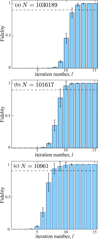
Figure 4: (Color online) Bar chart: the average of the fidelities between the reduced density matrix ρr(l)subscriptsuperscript𝜌𝑙𝑟\rho^{(l)}_{r} and the factors’ states ρfsubscript𝜌𝑓\rho_{f} are plotted versus the number l𝑙l of iterations in (a) N=1,030,189𝑁1030189N=1,030,189, (b) N=101,617𝑁101617N=101,617 and (c) N=10,961𝑁10961N=10,961. In each iteration, the fidelity Flsubscript𝐹𝑙F_{l} is taken at the time tlsubscriptsuperscript𝑡𝑙t^{*}_{l}, which is a uniformly distributed random number ranging from 0 to 2π/g2𝜋𝑔2\pi/g. Here the sample size is equal to 100 fidelities. The bars, which indicate the mean values, are shown in light blue. The error bars, which indicate the standard deviations, are shown in black. The dashed lines indicate that the fidelities attain 0.9.

Table 1 shows the relevant fidelity, the probability of obtaining the coherent state |αN(l)(tl)3subscriptketsubscriptsuperscript𝛼𝑙𝑁subscriptsuperscript𝑡𝑙3|\alpha^{(l)}_{N}(t^{*}_{l})\rangle_{3} with a magnitude |α(l)|=2superscript𝛼𝑙2|\alpha^{(l)}|=2, and the evolution time tlsubscriptsuperscript𝑡𝑙t^{*}_{l} for each iteration. Before starting the iteration, the initial fidelity F0subscript𝐹0F_{0} is very low: 2.883×1092.883superscript1092.883\times 10^{-9}. In the first few steps, the probabilities, Pr(El)subscript𝐸𝑙(E_{l}), of obtaining the coherent states, are about 101superscript10110^{-1}. We emphasize that now the probabilities Pr(El)subscript𝐸𝑙(E_{l}) are not extremely small, even when N𝑁N is large. This resolves the limitation of our previous proposal Ng . The probability of finding the factor’s state can be increased by 10 after a single iteration. After ten iterations, the fidelity can exceed 0.5. The fidelity can reach nearly one after two more iterations, while the probabilities P(El)𝑃subscript𝐸𝑙P(E_{l}) approach one. Also, we have explicitly shown that this method can factor a number of order of 106superscript10610^{6} with 12 iterations.

Since the evolution time tlsubscriptsuperscript𝑡𝑙t^{*}_{l} in Eq. (60) is a uniformly distributed random number from 0 to 2π/g2𝜋𝑔2\pi/g, it is necessary to study the effect of this randomly chosen time tlsubscriptsuperscript𝑡𝑙t^{*}_{l} to the performance of factoring. Now we study the averages of the fidelities Flsubscript𝐹𝑙F_{l} and probabilities Pr(El)subscript𝐸𝑙(E_{l}) of obtaining the coherent states. We also examine their standard deviations in each iteration.

In Fig. 4(a), we plot the average of the fidelities Flsubscript𝐹𝑙F_{l} versus the number l𝑙l of iterations. Here we take the sample size to be equal to 100 fidelities in each iteration. As shown in Fig. 4, the average of the fidelities is about 0.5 at the 10-th iteration. The fidelity is greater than 0.9 at the 12-th iteration. After 12 iterations, the mean values of the fidelities reach nearly one. The error bars, which indicate the standard deviations, are shown in the same figure. We can see that, after the 12-th𝑡th iteration, the standard deviations are relatively small compared to the mean values in each iteration.

We then plot the average of the fidelities Flsubscript𝐹𝑙F_{l} versus the number l𝑙l of iterations for N=10,1617𝑁101617N=10,1617 and 10,961 in Fig. 4(a) and (b), respectively. The fidelities exceed 0.9 after the 10-th iteration for N=101,617𝑁101617N=101,617 and the 8-th iteration for N=10,961𝑁10961N=10,961. The numerical results in Fig. 4 show that the required number of iterations increases logarithmically with N𝑁N for which the fidelity is greater than 0.9.

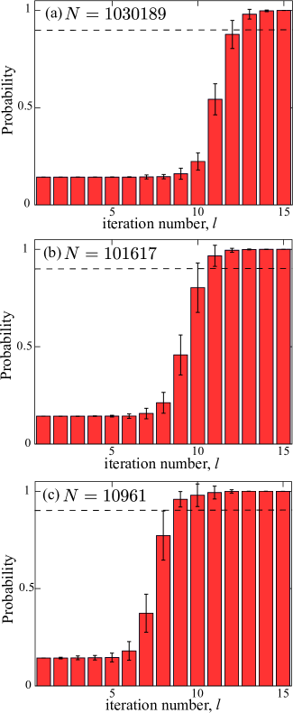
In Fig. 5(a), the average of the probabilities Pr(El)subscript𝐸𝑙(E_{l}) of obtaining the coherent states is plotted versus the number l𝑙l of iterations. In the first ten iterations, the probabilities Pr(El)subscript𝐸𝑙(E_{l}) are about 0.1. Then, it increases and saturates around one after 13 iterations. Moreover, these standard deviations are much smaller than the mean values of Pr(El)subscript𝐸𝑙(E_{l}). This means that the statistical effect of the time tlsubscriptsuperscript𝑡𝑙t^{*}_{l} is small on the performance of quantum factorization.

In Fig. 5(b) and (c), the average of the probabilities Pr(El)subscript𝐸𝑙(E_{l}) of obtaining the coherent states are plotted versus the number l𝑙l of iterations for N=101,617𝑁101617N=101,617 and N=10,961𝑁10961N=10,961, respectively. The probabilities are greater than 0.9 after the 11-th iteration for N=101,617𝑁101617N=101,617 and the 9-th iteration for N=10,961𝑁10961N=10,961. Therefore, the results show that the number of iterations (Pr(El)0.9subscript𝐸𝑙0.9(E_{l}){\geq}0.9) also logarithmically scales with N𝑁N.

Refer to caption
Figure 5: (Color online) Bar chart: the average of the probabilities of obtaining the coherent states |αN(l)(tl)3subscriptketsubscriptsuperscript𝛼𝑙𝑁subscriptsuperscript𝑡𝑙3|\alpha^{(l)}_{N}(t^{*}_{l})\rangle_{3} are plotted versus the number l𝑙l of iterations in (a) N=1,030,189𝑁1030189N=1,030,189, (b) N=101,617𝑁101617N=101,617 and (c) N=10,961𝑁10961N=10,961. In each iteration, the probability is taken at the time tlsubscriptsuperscript𝑡𝑙t^{*}_{l} which is a uniformly distributed random number from 0 to 2π/g2𝜋𝑔2\pi/g. Here the sample size is taken to be 100 probabilities. The bars, which indicate the mean values, are in red. The error bars, which indicate the standard deviations, are shown in black. The dashed lines indicate that the probabilities attain 0.9.

V Limitations and problems

We have introduced an amplitude-amplification method for factoring integers by using three coupled harmonic oscillators. However, this method requires an exponential amount of resources for implementation. This means that the required resource is of order of O(N)𝑁({N}), where N𝑁N is the input size. This means that this approach cannot provide any speed-up compared to classical algorithms. We discuss these two limitations in the following subsections.

V.1 Exponential energy resource

First, this approach requires an exponential amount of energy resource to encode a number N𝑁N onto the state of a single harmonic oscillator. For example, to factorize a number N𝑁N, two harmonic oscillators are used for encoding O(N3/2)𝑂superscript𝑁32O(N^{3/2}) possible states of trial factors. The energy EωO(N3/2)similar-to𝐸Planck-constant-over-2-pi𝜔𝑂superscript𝑁32E~{}\sim~{}\hbar{\omega}O(N^{3/2}) is thus required, where ωω1,2𝜔subscript𝜔12\omega\approx{\omega_{1,2}} are the frequencies of the harmonic oscillators 1 and 2. The required energy scales with the size of the input number N𝑁N. Therefore, the energy becomes enormous when the encoded number is large. This encoding method becomes impractical when a large input number is used. This problem may be resolved by using another encoding method. For example, the number could be encoded either onto qubit or qudit states. Thus, the required energy for encoding numbers could be reduced.

V.2 Exponential size of the ensemble

Second, this method requires an exponential size of the ensemble of harmonic oscillators for an input N𝑁N. In each iteration, it is necessary to abandon a large number of harmonic oscillators after each conditional measurement. The number of abandoned oscillators is proportional to the failure probability of obtaining conditional measurement of the coherent states in each step. Therefore, a number at least of order of O(N)𝑁({N}) harmonic oscillators are needed in order to complete the entire procedure. This requires an exponential resource for preparing the ensemble of oscillators. This approach may be improved by employing efficient methods for preparing the ensembles.

VI Conclusions

We have presented an amplitude-amplification method by repeatedly using the nonlinear interactions between the harmonic oscillators and non-orthogonal measurements. We have shown that this approach can be used for factoring integer, and the factors of an integer N𝑁N can be obtained, with a high probability, by using a number of iterations LO(log2N)similar-to𝐿𝑂subscript2𝑁L\sim{O(\log_{2}{N})}. We have numerically studied an example for factoring N=1,030,189𝑁1030189N=1,030,189, respectively. We have shown how to factorize an integer of order of O(106)𝑂superscript106O(10^{6}) within 12 iterations. In each iteration, the probability of obtaining this coherent state, with the rotation frequency being proportional to N𝑁N, is not less than 0.1. By comparing examples with N=101,617𝑁101617N=101,617 and N=10,961𝑁10961N=10,961, we have shown that the required number of iterations increases logarithmically with N𝑁N.

However, using coupled harmonic oscillators, this method requires the use of an exponential amount of resources, i.e., exponential energy and ensemble size. Thus, this approach becomes impractical for large input sizes. We hope that the resolutions could be proposed to overcome the problems of this approach.

Also, we stress that the nonlinear interactions between the coupled oscillators and conditional measurements are essential in this approach. By appropriately controlling nonlinear interactions between the coupled harmonic oscillators, the functions with integer inputs can be evaluated in a single operation. To implement this approach, it is necessary to engineer “many-body” interactions of the system of harmonic oscillators. For example, to perform quantum factorization, it is required to generate “three-body” interactions between the harmonic oscillators. We have briefly discussed the possible implementations in Ref. Ng . One of the promising candidates is neutral atoms or polar molecules trapped in optical lattices Buchler ; Johnson ; Will . The “three-body” interactions can be tuned by external fields Buchler ; Johnson .

Acknowledgements.
FN acknowledges partial support from the Army Research Office, JSPS-RFBR contract No. 09-02-92114, Grant-in-Aid for Scientific Research (S), MEXT Kakenhi on Quantum Cybernetics, and the Funding Program for Innovative R&D on Science and Technology (FIRST).

References

  • (1) R. Feynman, Int. J. Theor. Phys. 21, 467 (1992).
  • (2) D. Deutsch, Proc. R. Soc. London, Ser. A 400, 97 (1985).
  • (3) A. Ekert and R. Jozsa, Rev. Mod. Phys. 68, 733 (1996).
  • (4) M. A. Nielsen and I. L. Chuang, Quantum Computation and Quantum Information (Cambridge University Press, Cambridge, 2000).
  • (5) P. Kaye, R. Laflamme and M. Mosca, An Introduction to Quantum Computing (Oxford University Press, Oxford, 2007).
  • (6) I. Buluta and F. Nori, Science 326, 108 (2009).
  • (7) I. Buluta, S. Ashhab and F. Nori, arXiv:1002.1871.
  • (8) J. Q. You, F. Nori, Physics Today 58 (11), 42 (2005).
  • (9) A. M. Childs and W. van Dam, Rev. Mod. Phys. 82, 1 (2010).
  • (10) P. Shor, Proc. 35th Ann. Symp. Found. Comp. Sci. (IEEE Comp. Soc. Press, Los Alamitos, California, 1994), p. 124.
  • (11) L. K. Grover, Phys. Rev. Lett., 79, 325 (1997).
  • (12) H. T. Ng and F. Nori, arXiv:1007.4338.
  • (13) L. A. Wolsey, Integer Programming (Wiley-Interscience, 1998).
  • (14) C. H. Bennett, E. Bernstein, G. Brassard and U. Vazirani, SIAM J. Comput. 26, 1510 (1997).
  • (15) F. S. Hillier and G. J. Lieberman, Introduction to Operations Research 9th revised edition, (McGraw-Hill, 2009).
  • (16) S. M. Barnett and P. M. Radmore, Methods in Theoretical Quantum Optics (Oxford University Press, Oxford, 2002).
  • (17) H. M. Wiseman and G. J. Milburn, Quantum Measurement and Control (Cambridge University Press, Cambridge, 2010).
  • (18) A. Uhlmann, Rep. Math. Phys. 9, 273 (1976)
  • (19) R. Jozsa, J. Mod. Opt. 41, 2315 (1994).
  • (20) H. P. Büchler, A. Micheli and P. Zoller, Nature Phys. 3, 726 (2007).
  • (21) P. R. Johnson, E. Tiesinga, J. V. Porto and C. J. Williams, New J. Phys. 11, 093022 (2009).
  • (22) S. Will, T. Best, U. Schneider, L. Hackermüller, D.-S. Lühmann and I. Bloch, Nature 465, 197 (2010).