Replica Exchange Monte Carlo applied to Hard Spheres
Abstract
In this work a replica exchange Monte Carlo scheme which considers an extended isobaric-isothermal ensemble with respect to pressure is applied to study hard spheres (HS). The idea behind the proposal is expanding volume instead of increasing temperature to let crowded systems characterized by dominant repulsive interactions to unblock, and so, to produce sampling from disjoint configurations. The method produces, in a single parallel run, the complete HS equation of state. Thus, the first order fluid-solid transition is captured. The obtained results well agree with previous calculations. This approach seems particularly useful to treat purely entropy-driven systems such as hard body and non-additive hard mixtures, where temperature plays a trivial role.
I Introduction
The replica exchange Monte Carlo (REMC) method Lyubartsev91 ; Marinari92 , also called parallel tempering Yan99 , was derived to achieve good sampling of systems that present a free energy landscape with many local minima Bittner08 ; Frenkel . It consists on simulating several replicas of the same system at different thermodynamic states, and allowing for replica exchanges (swap moves). Thus, it is possible to implement an ergodic walk through free energy barriers connecting disjoint configuration subspaces by defining a set of close enough thermodynamic states. Although it has been developed at the end of the last century Lyubartsev91 ; Marinari92 , its acceptance is already high due to its clearness, simplicity, and its wide applicability. Proof of that is its employment to find zeolite structures Falcioni99 , to study different conformations of proteinsHernandez08 , and to access phase equilibrium of many single and multicomponent systems Fiore08 ; Imperio06 ; Arnold08 .
Most frequently, the REMC technique is employed to sample an extended canonical ensemble in temperature. Thus, those replicas having larger temperatures are capable of escaping from local free energy minima, where the pair potential attraction of the constituting particles plays a key role. When the free energy minima are mainly dictated by the entropic term, i. e., by the excluded volume repulsive interactions Fortini06 ; Odriozola08 ; Jimenez08 , enlarging the temperature has a small effect. In other words, the benefits of the method become restricted. This is especially true when dealing with hard body systems (purely entropy-driven systems) such as hard spheres (HS), rods, plates, polymers, and non-additive hard mixtures, since they constitute limiting cases where the pair interactions are repulsive only and the temperature plays a trivial (null) role. Thus, it is not very surprising that the REMC technique has not been applied yet to this kind of systems. To do this, an alternative would be performing the ensemble extension in pressure instead of temperature, to provide the particles more freedom to rearrange as the volume expands. This idea is tested in this work for HS.
It is well known that fluid-solid transitions represent a challenge for computational science Wilding00 ; Noya08 . Most techniques which properly work for accessing liquid-gas transitions have problems at very high densitiesFrenkel . Therefore, the freezing and melting points are at least difficult to determine Wilding00 . Indeed, for the HS model, simulations have recently produced an accurate determination of the freezing and melting point theoretically reported in the sixties Wilding00 ; Noya08 . That is despite the intense study of HS through the past decades, and the fact that the HS model was one of the first systems ever studied by computer simulations Rosenbluth54 ; Wood57 ; Alder57 . Additionally, the HS model shows a high density metastable branch ending at the random close package density Rintoul96 , which adds difficulty for sampling from equilibrium.
The aim of this study is to show that the REMC can be successfully applied to study hard body systems. Hence, the REMC is used by performing a NPT ensemble extension on pressure and applied to HS. The paper is structured as follows. Sec. I is this brief introduction. Sec. II describes the employed algorithm. Results are given in Sec. III. Finally, in Sec. IV conclusions are drawn.
II Numerical Method
As mentioned, in the parallel tempering scheme identical replicas are considered, each following a typical canonical simulation. However, a different temperature is set for each one of them. Thus, an extended ensemble can be defined so that its partition function is , being the partition function of ensemble at temperature , number of particles , and volume . The existence of this extended ensemble justifies the introduction of swap trial moves between any two ensembles (each ensemble is sampled by only one replica at a time), whenever the detail balance condition is satisfied. If all swap trials have the same a priori probability of being performed, the swap acceptance probability becomes
| (1) |
where is the reciprocal temperature of replica , is the Boltzmann’s constant, and is the energy of replica . Hence, by introducing these swap trials, a particular replica seals through many temperatures allowing it to overcome free-energy barriers. Additionally, sampling on particular ensembles is not disturbed but enriched by the different contributions of the replicas.
For studying systems where excluded volume interactions dominate, it may be convenient to allow the replicas to expand for destroying any local order. Additionally, in the case of a HS system (or any other purely entropy-driven model) an extended ensemble in temperature is pointless, since this variable does not affect the system structure. For that purpose, the extended ensemble is defined as , being the partition function of the isobaric-isothermal ensemble of system , at pressure , fixed temperature , and number of particles (note that the extension is in pressure; an isobaric-isotermal extension in temperature applied to a Lennard Jones system is given by Okabe et. al. Okabe01 ). This extended ensemble can be sampled by performing standard simulations on each replica, which implies typical particle displacement trials and volume change trials. Notwithstanding, the sampling can be significantly improved by introducing swap trials between neighboring ensembles. Again, the only restriction is that the detail balance condition must prevail to guaranty the correct sampling. One way of achieving this is by setting equal all a priori probabilities of choosing the different adjacent pairs of replicas, and accounting for the following acceptance probability
| (2) |
where is the volume difference between replicas and . It should be noted that the ensemble extension in pressure leads to a simple acceptance rule where energy terms vanish.
For , and so, the acceptance rule tends to order the replicas by volume size (lower volumes at higher pressures). For , depends on the absolute value of the pressure differences of the adjacent ensembles, . A decrease of leads to a larger acceptance probability. Consequently, adjacent pressures should be close enough to provide large exchange acceptance rates between neighboring ensembles. This is particularly important where a phase transition takes place (characterized by large ), which generally leads to a bottleneck of the swap acceptance rate. Additionally, the swap acceptance rate also depends on the system size. Larger system sizes produce narrower distribution of densities (volumes) for a given pressure, providing smaller overlap regions between adjacent ensembles. Hence, a larger system size leads to a decrease of the swap acceptance probability. Finally, in order to take a good advantage of the method, the replica at the lowest pressure must assure large jumps in configuration space, so that the higher pressure ensembles can be sampled from disjoin configurations.
In this work, cubic boxes of initial side are considered. These boxes are filled by randomly placing hard spheres of diameter . The initial density, , is set to 0.30 for all replicas. A geometrically increasing pressure, , is set from approximately 2 to 100 , and arbitrarily assigned to the replicas. Where the fluid-solid transition is expected, intermediate pressures are added (the total number of replicas equals the number of different pressures). An optimal allocation of replicas should lead to a constant swap acceptance probability for all pair of adjacent ensembles Rathore05 . Two experiments were done, one with and the other with . The simulation starts by following the trial moves above described (see the appendix for details).
Sampling consists on measuring densities, radial distribution functions, average number of neighbors, and the order parameter , as a function of the pressure. The average number of neighbors, , is computed accounting for all pairs having a center-center distance smaller than (the vectors joining the centers of these pairs are named bonds). The order parameter is defined as Steinhardt83 ; Rintoul96
| (3) |
where is the average over all bonds and configurations of the spherical harmonics of the orientation angles and (these are the polar angles of the bonds measured with respect to any fixed coordinate system, since is invariant). should go to zero for a completely random system of a large number of points, following Rintoul96 .
III Results
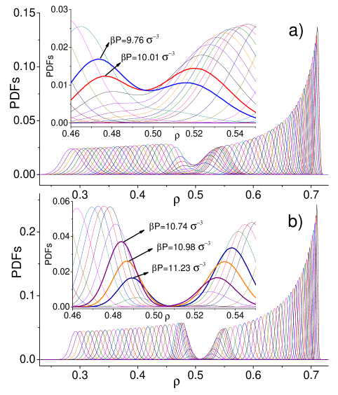
Figure 1 a) shows the probability density functions, PDFs, to find a replica at a given density for all pressures and for . The 70 PDFs correspond to the different assigned pressures. In general, the PDFs are bell-shaped and centered on a maximum which location depends on the assigned pressure. The leftmost curve corresponds to the lowest pressure (2.16 ) and the rightmost to the highest one (100 ). As pressure increases, the curves narrow and shift to the right producing larger densities (the narrowing is very pronounced for high pressures). The exception occurs for densities close to , where the PDFs split yielding bimodal distributions. At , the replicas produce few configurations, and the bimodals yield a local peak below 0.49 and another above 0.51. Thus, a jump on density from to is produced for , pointing out the well known HS fluid-solid transition. The inset of figure 1 a) zooms in the density region around 0.5, where the PDFs are much clearly seen. There it is shown the pressures that correspond to the PDFs which are closer to the transition.
The PDFs obtained for are shown in figure 1 b). As expected, similar trends are seen. That is, PDFs are bell-shaped, they narrow and shift toward larger densities for increasing pressure, and they turn bimodal for densities close to 0.5. Nevertheless, PDFs are higher (approximately two times higher) and (consequently) narrower than for . Also the bimodal distributions become sharper producing interpeak regions rarely visited by the replicas. In fact, for the PDFs are practically zero. In other words, the HS fluid-solid transition turns more evident by increasing the system size. As in figure 1 a), the inset of figure 1 b) zooms in the corresponding PDFs. From there it can be estimated the transition occurring at with and . Thus, the transition occurs at a higher pressure and shifts to larger densities for increasing the system size. The gap between the fluid and solid densities also enlarges.
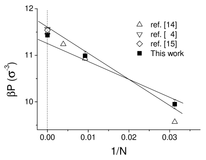
The data obtained for small values can be extrapolated to estimate the HS bulk coexistence pressure, fluid density, and solid density. These are , 0.492 0.004, and 0.545 0.004, respectively. These values are in good agreement with previous calculations Frenkel ; Wilding00 ; Noya08 . Figure 2 shows the extrapolation for the coexistence pressure, and a comparison with data reported by different authors. As can be seen, the obtained agreement is good, suggesting that the RECM method works properly for capturing the HS fluid-solid transition.
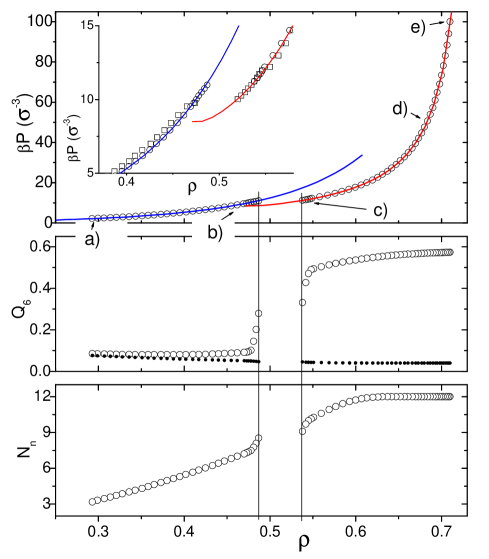
The topmost plot of figure 3 is built by plotting the pressure as a function of the most frequent density for . It is also shown as a red line a Padé approximation to data obtained from the HS fluid state Speedy97 , and as a blue line a fit to the HS face cubic centered (FCC) solid state Speedy98 , both data series obtained by means of simulations. As an inset, it is shown a zoom in of the same data for the coexistence, where there were added the data obtained for . Both curves here reported, for the fluid and solid states, well agree with the equation of state given by Speedy. This confirms the good behavior of the REMC ensemble extension on pressure. Nevertheless, there is a slight deviation from the FCC curve of Speedy close to the transition. This may signal the presence of hexagonal close-packed (HCP) arrangements and even hybrid FCC-HCP structures.
The middle and bottommost plots of figure 3 show the order parameter, , and the number of first neighbors, , as a function of , respectively. The middle plot also shows as bullets the value of for completely space-uncorrelated particles. As expected, is small for the fluid region, pointing out the practical absence of angular order. However, it is always somewhat larger than the value of for a random system. The difference between these two values diminishes for decreasing . On the other hand, reaches for , which is slightly lower than the value of the FCC arrangement, , and well above the corresponding value of the HCP structure, . This signals that only replicas approaching the FCC lattice are allowed for the highest applied pressures. This is not surprising since 108 identical spherical particles can be perfectly packed on a cubic box on a FCC lattice, but cannot on a HCP lattice. Thus, the system is being forced to promote FCC over HCP at high pressures. For lower but still over the coexistence pressures, is close to 0.5, suggesting that both lattices and their hybrids contribute to the average. It should be noted that sharply increases at the fluid-solid transition. Thus, it can be employed to detect any trace of local angular order. This was shown to be much more reliable than the radial distribution function peak that develops close to 1.5 Rintoul96 . Finally, monotonically increases with . It also shows a sharp increase at the coexistence, although less pronounced than for . At large densities reaches 12, which is the largest possible HS coordination number, as it is well known.
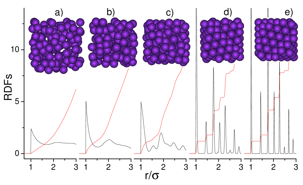
The radial distribution functions (RDFs) and their corresponding integrals for cases a), b), c), d), and e) pointed out in figure 3 are plotted in figure 4. Cases a) and b) correspond to the fluid phase, and the other three correspond to the solid phase. Case a) shows the typical low density liquid structure, where a relatively small contact value is developed and the second shell of neighbors is poorly seen. As the density increases, case b), the RDF shows a larger contact value (two times larger than case a)), and a well defined second shell of neighbors. This case corresponds to a liquid close to the coexistence. Slightly above the coexistence, the RDF looks like case c). Here a small peak appears at , whereas the valley in-between this peak and the contact one deepens. Other peaks also form at larger distances. For density values close to , case d), the RDF develops the full character of a crystal. That is, peaks are very high and narrow, and valleys turn practically zero. The integral (red line) of this case highlights this fact, since it shows a step-like behavior. The first step reaches 12, pointing out the first shell coordination number (integral of the peak at ), the second yields 18 (), the third 42 (), and the fourth 54 (), what corresponds to the FCC structure. Nonetheless, a small shoulder appears at the left of the fourth peak (), suggesting the existence of few configurations having a HCP structure. For larger densities, case e), this shoulder disappears and a practically pure FCC RDF is observed.
IV Conclusions
This work shows that a replica exchange Monte Carlo scheme can be successfully applied to study hard spheres at high densities. For that purpose, an extension of the isobaric-isothermal ensemble with respect to pressure is used. The algorithm employs standard particle trial displacements and volume changes together with replica exchanges (swap moves). These easy to implement trials are shown to be enough for capturing the fluid-solid transition of hard spheres and the solid equilibrium branch for small systems. The obtained results well agree with previous calculations. The principal idea behind this scheme is to increase the particles mobilities by decreasing the pressure (expanding the volume), so that systems characterized by large excluded volume contributions are able to visit disjoint configurations of configurational space. This approach seems particularly useful to deal with purely entropy-driven systems such as hard body and non-additive hard mixtures, where temperature plays a trivial role.
V Appendix- Simulation Details
Once the boxes are filled with the spheres and are assigned the corresponding different pressures, the algorithm starts performing the trials. As mentioned, they are: particle displacements, volume changes, and swap moves. The probability for selecting a particle displacement trial (in any of the boxes), , is fixed to . The probabilities for selecting a volume change trial, , and a swap trial, , are and . Here, is a weight factor fixed to . Additionally, the probability of performing a particle displacement trial and a volume change trial in a replica enlarges as it is closer to the fluid-solid transition pressure. These probabilities are 10 times larger for the central replica than for those having the highest and the lowest pressures. All particles of a given replica have the same a priori probability of being selected to perform a displacement trial. The same is true for selecting a pair of adjacent replicas to attempt a swap move (there are pairs). Thus, a random number homogeneously distributed in [0,1] is generated in order to determine the type of trial to be performed. In case of selecting a particle displacement, the algorithm provides the replica and the particle for applying the trial. In case of a volume change trial, it identifies the replica; and in case of a swap trial, the algorithm gives the adjacent replicas to apply it. Next, another random number is generated to produce a second trial. If these two trials are independent the one another (for instance, they are particle trials on different replicas) the algorithm generates a third trial (note that these trials are not being applied yet). This procedure is repeated until the last trial cannot be performed independently of the others (for instance, a particle displacement trial on a replica in which a volume change trial must be previously performed). This way, the algorithm have randomly selected a given number of independent trials to be applied on the replicas. Immediately after, the algorithm parallelizes (in two threads, since a dual core desktop is used), and the trials are done. The last generated trial (which was not yet performed) becomes now the first trial to be applied on the following series of trials. This procedure is followed to strictly preserve the detail balance condition (to build a symmetric transition matrix) while performing a parallelization. Verlet lists are employed for saving CPU time (note that the saving can be quite large since replicas at high pressures rarely update their lists).
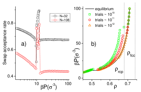
Sampling is not performed for the first trials (initializing procedure). During this process, the maximum displacements of particles and maximum volume changes for each pressure are tuned to yield acceptance rates close to 0.4. Thus, particle maximum displacements and maximum volume changes of ensembles having high pressures turn smaller than those associated to ensembles having low pressures. Once this is done, all maximum displacements (one for each pressure) and maximum volume changes (also one for each pressure) become fixed. trials are then employed to yield the data shown in the body of the article (equilibrium sampling).
The acceptance rates obtained for the swap trials are shown in Fig. 5 a) as a function of the pressure, . As expected, the acceptance rates for the smaller system () are, in general, larger than the ones obtained for the larger system (). This is a consequence of the larger overlaps of the distributions. In both cases the values are above the recommended acceptance rate of 0.2 Rathore05 . For , the acceptance rate is practically constant. On the contrary, for , the acceptance rate increases with decreasing . This means that for the fluid region, should be reduced more than geometrically for optimization purposes. For , the acceptance rate increases. This is due to the fact that smaller pressure differences are set between the adjacent ensembles to compensate the natural decrease of the acceptance rate at the fluid-solid transition. Note that more than the necessary replicas are added in order to decrease the error of the coexistence pressure (the natural decrease of the acceptance rate is overcompensated). In addition, this study is focussed on yielding a detailed sampling of a large range. To acquire equilibrium data from a high pressure system only, many fewer replicas would be required (the optimal swap acceptance rate is close to when temperature is employed as the thermodynamic variable of ensemble extension Rathore05 ).
Figure 5 b) shows the evolution of the pressure versus density plot with the number of performed trials during the initializing procedure (). For trials, the sampling yields a curve at which may correspond to the random close packing (RCP) metastable branch. There are also 5 replicas which reached the equilibrium state (since they crystalized, they were pushed towards the highest pressure region). Another one, producing the point laying on the dotted line, may correspond to a partially crystalized structure. Assuming this well defined curve corresponds to the RCP branch, is obtained from Rintoul96 . This is larger than the reported value of Rintoul96 , suggesting that some degree of crystallization is already taking place on the replicas at high pressure. This is in fact confirmed by the analysis (not shown). As the initializing process advances, the degree of crystallization augments and the high pressure curve shifts approaching the equilibrium branch ( also enlarges). For trials, the curve practically yields the equilibrium branch. From here on, only those replicas having a large degree of crystallinity are able to access the high pressure region. At this point, the initializing procedure ends and the sampling from equilibrium process starts.
References
- (1) A. P. Lyubartsev, A. A. Martsinovski, S. V. Shevkunov, and P. N. Vorontsov-Velyaminov, J. Chem. Phys. 96, 1776 (1991)
- (2) E. Marinari and G. Parisi, Europhys. Lett. 19, 451 (1992)
- (3) Q. L. Yan and J. J. de Pablo, J. Chem. Phys. 111, 9509 (1992)
- (4) E. Bittner, A. Nußbaumer, and W. Janke, Phys. Rev. Lett. 101, 130603 (2008)
- (5) D. Frenkel and B. Smit, Understanding molecular simulation (Academic, New York, 1996)
- (6) M. Falcioni and M. W. Deem, J. Chem. Phys. 110, 1754 (1999)
- (7) J. Hernández-Rojas and J. M. G. Llorente, Phys. Rev. Lett. 100, 258104 (2008)
- (8) C. E. Fiore, Phys. Rev. E. 78, 041109 (2008)
- (9) A. Imperio and L. Reatto, J. Chem. Phys. 124, 164712 (2006)
- (10) A. Arnold and C. Holm, Eur. Phys. J. E 27, 21 (2008)
- (11) A. Fortini and M. Dijkstra, J. Phys.: Condens. Matter 18, L371 (2006)
- (12) G. Odriozola, F. Jiménez-Ángeles, and M. Lozada-Cassou, J. Chem. Phys. 129, 111101 (2008)
- (13) F. Jiménez-Ángeles, Y. Duda, G. Odriozola, and M. Lozada-Cassou, J. Chem. Phys. 129, 111101 (2008)
- (14) N. B. Wilding and A. D. Bruce, Phys. Rev. Lett. 79, 3002 (1997)
- (15) E. G. Noya, C. Vega, and E. de Miguel, J. Chem. Phys. 128, 154507 (2008)
- (16) M. N. Rosenbluth and A. W. Rosenbluth, J. Chem. Phys. 22, 881 (1954)
- (17) W. W. Wood and J. D. Jacobson, J. Chem. Phys. 27, 1207 (1957)
- (18) B. J. Alder and T. E. Wainwright, J. Chem. Phys. 27, 1208 (1957)
- (19) M. D. Rintoul and S. Torquato, J. Chem. Phys. 105, 9258 (1996)
- (20) T. Okabe, M. Kawata, Y. Okamoto, and M. Masuhiro, Colloid Polym. Sci. 335, 435 (2001)
- (21) N. Rathore, M. Chopra, and J. J. de Pablo, J. Chem. Phys. 122, 024111 (2005)
- (22) P. J. Seinhardt, D. R. Nelson, and M. Ronchetti, Phys. Rev. B. 28, 784 (1996)
- (23) R. J. Speedy, J. Phys.: Condens. Matter 9, 8591 (1997)
- (24) R. J. Speedy, J. Phys.: Condens. Matter 10, 4387 (1998)