Do your volatility smiles take care of extreme events?

Abstract

In the Black-Scholes context we consider the probability distribution function (PDF) of financial returns implied by volatility smile and we study the relation between the decay of its tails and the fitting parameters of the smile. We show that, considering a scaling law derived from data, it is possible to get a new fitting procedure of the volatility smile that considers also the exponential decay of the real PDF of returns observed in the financial markets. Our study finds application in the Risk Management activities where the tails characterization of financial returns PDF has a central role for the risk estimation.

I Introduction

Financial derivatives are the modern financial instruments that are used in many activities and for different purposes: mitigating risk exposure, speculation and arbitrage, trading strategies, providing leverage, etc. Knowing the fair value of such kind of contracts is not, generally, an easy task and it is of crucial importance, for example, for the correct evaluation of a portfolio of financial instruments and the related risks.
One of the simplest “products” on the derivative financial market is the European call (put) option Hull ; Wilmott . Considering the risk neutral approach, the price of the European call option, $C\equiv C(S_{T},K,T,r)$, is defined by

$$C=e^{-rT}\int_{K}^{\infty}(S_{T}-K)P(S_{T})dS_{T},$$ (1)

where $S_{T}$ is the stock price at time $t=T$, $K$ is the strike price of the option, $T$ is the expiration time (time to maturity) of the option, $r$ is the interest rate and $P(S_{T})\geq 0$ is the distribution function of the stock prices in a “risk-neutral world” ($\int_{0}^{\infty}P(S_{T})dS_{T}=1$).

Eq. (1) is too general because it does not make any hypothesis on the underlying stock price distribution function, $P(S_{T})$. To calculate explicitly the option price, $C$, using Eq. (1), one can assume that the distribution function, $P(S_{T})$, is log-normal, so that, for the logarithmic return deprived of the risk-free component, $x=\ln(S_{T}/S(t))-r(T-t)$, the distribution is normal:

$$P(x)=\frac{1}{\sqrt{2\pi\sigma^{2}(T-t)}}\exp\left[-\frac{(x+\sigma^{2}(T-t)/2)^{2}}{2\sigma^{2}(T-t)}\right],$$ (2)

where $S(t)$ is the stock price at time $t$ and $\sigma$ is the stock price volatility. For seek of simplicity, in the following we consider $t=0$ and we define $S_{0}\equiv S(t=0)$.

Using the Eqs. (1), (2) it is possible to get an explicit expression for the price of the European call option:

$$C^{BS}=S_{0}N(d_{1})-Ke^{-rT}N(d_{2}),$$ (3)

where

$$\begin{array}[]{ccc}d_{1}&=&\displaystyle\frac{\ln(S_{0}/K)+(r+\sigma^{2}/2)T}{\sigma\sqrt{T}},\\ &&\\ d_{2}&=&d_{1}-\sigma\sqrt{T},\\ &&\\ N(x)&=\displaystyle&\frac{1}{\sqrt{2\pi}}\int_{-\infty}^{x}\ dz\ e^{-{z^{2}}/{2}}.\\ &&\\ \end{array}$$ (4)

The Eq. (3) gives an analytical solutions for the European call option pricing and it is the main results of the Black-Scholes (BS) theory about option pricing Black .

The distribution function (2) follows from a stochastic model for stock prices,

$$dS=rSdt+\sigma Sdz,$$ (5)

where $dz$ is a Wiener increment winer_note . It can be shown it is never optimal to exercise an American call option on a non-dividend-paying stock early Hull ; Bouchaud ; therefore Eq. (3) can also be used to estimate the fair value for this kind of options.
Since 1973, when the BS model was published Quantitative Finance became a prominent aspect in many banks and financial institutions activities and a lot of new, more realistic models were developed for the option pricing Heston ; Hagan . These new models are currently implemented and used by traders and risk managers of many financial institutions and it could seem that the BS model is by now outdated and irrelevant for financial applications. On the contrary, because of its simplicity and the small number of parameters, BS model is still a benchmark, used by practitioners in many situations where getting a reliable calibration of parameters of more complex models could be unattainable in practice. Simplicity and a sort of reluctance to changes explain, in our opinion, the reason why, after about 37 years from its publication, BS model is still used by practitioners and justify the importance of our study to get a correct calibration procedure for the volatility smile (VS) effect also from a theoretical point of view. In a recent paper Spada it is shown a new calibration procedure that can be obtained using an adiabatic approach to avoid arbitrage opportunities. The term “adiabatic” comes from comes from statistical physics and is related to the slowness of the variation of a parameter $\lambda$ that specifies the properties of a system or an external field. In fact from a physical point of view, it can be shown that if in a system one introduces a small perturbation ($\lambda$) compared to the characteristics period of the motion $T$, namely:

$$T\frac{d\lambda}{dt}\ll\lambda$$ (6)

the rate of the change of the energy of the system will be also small Landau . In the same spirit we assume that our parameter $\lambda$ is represented by the implied volatility $\sigma$ and we study how to characterize PDF of returns with a small perturbation of the parameter $\sigma$ to get a suitable description of actual data, coherent from a theoretical point of view. In particular, in the following, it is shown the importance of this calibration procedure from the risk management point of view and its relevance in the risk estimation.
The rest of the paper is organized as follows.

In Section II, we analyze the volatility smiles from Foreign Exchange (FX) market data and we propose a suitable function to fit it. We also find a relation between the fitting parameters that holds for every symmetric smile that help us to identify the real independent variables of our system. Using this relation we determine a suitable range of parameters for our simulation.

In Section III we outline the relation between VS and PDF of returns and we stress the importance of getting a suitable fit for the VS for the risk estimation

In Section IV, we study the relation between the parameters of our volatility smile function and the decay of the PDF of financial returns and we find an equation to describe this kind of behavior.

In Section V, we show how to get a more reliable fit of the volatility smile, considering the exponential decay of the returns PDF. To do this we exploit the relation between the standard deviation of an exponential distribution and its decay. Finally, in Section VI we present our conclusions.

II Volatility smile: Analysis of actual market data

Typically, traders on option markets and practitioners consider the BS model as a zeroth order approximation that takes into account the main features of options prices. To get a pricing closer to the actual data, they consider the volatility as a parameter that can be adjusted considering the inverse problem given by Eq. (3) and the real price of call and put options. In this way a more reliable value of the volatility (implied volatility) can be obtained and it can be used to price more complex options for which analytical solutions are not available. The value of the implied volatility depends on the value of the strike, $K$, in a well-known characteristic curve called the smile volatility (typically for foreign currency options) whose shape is approximately parabolic and symmetric, or skew volatility (typically for equity options) when asymmetric effects dominate Risk ; Tompkins ; Toft ; Campa .

An intuitive explanation of this shape can be found if an actual returns distribution is considered. In fact, it is well known that the tails of the returns PDF are not Gaussian but exhibit a power law decay (fat-tails) Sorn ; Stan or exponential decay Heston . On the contrary, BS model assumes that the PDF of returns is Gaussian thus underestimating the actual probability of rare events. To compensate for this model deficiency, one has to consider the greater implied volatility for strike out of the money than for strike at the money.

In this paper we focus our attention on the VS of foreign currency options and we neglect the skew effect Kirch . To perform our analysis we consider the volatility smile as a function of the $\Delta$ of the option (defined by Eq. (7)), the time to maturity, $T$, and the currency considered. We consider specific days, for which volatility is not affected by the skew effect, and we use Bloomberg as data provider. In the BS model, the $\Delta$ of a call options is defined as:

$$\Delta=\frac{\partial C}{\partial S_{T}}=\displaystyle erf(d_{1}),$$ (7)

Inverting this relation is possible to get an expression for $x$:

$$x=\sigma^{2}/2T-\sigma\sqrt{T}\ erf^{-1}(\Delta),$$ (8)

where $erf^{-1}(x)$ is the inverse of the error function.

Figure 1: Typical VS and the relative fit obtained with Eq.  (9). The parameters of the fit are: $g=0.1758(5)$, $\chi=1.20(9)$, $n=0.00030(9)$. We get the real data using Bloomberg provider and they refer to the AUDUSD currency with time to maturity $T=1/365$ years.

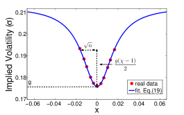
In Fig. 1 we show an example of VS in terms of our variables and a suitable fit given by the function:

$$\sigma(x)=g\left[1+(\chi-1)\frac{(x+g^{2}T/2)^{2}}{(x+g^{2}T/2)^{2}+n}\right]$$ (9)

where $g,\chi,n$ are fitting parameters. In this case, $g$ represents the minimum of the volatility smile, $\sqrt{n}$ is the half width at the half height, while $g(\chi-1)$ represents the height of the smile. In particular $\chi$ is the ratio between the limiting value of $\sigma$ as $x$ approaches $\infty$ and $g$ . In this way the variation of $\sigma$ is bounded between $g$ and $g\chi$. In the light of the intuitive explanation of the volatility smile proposed above and since from (2) it follows that the average value,

$$\langle x\rangle=-\frac{\sigma^{2}T}{2},$$ (10)

one expects that the minimum of the implied volatility occurs at $x=-g^{2}T/2$ as required by our fitting function.

We repeat the fitting procedure considering the volatility smile for different days, currencies and time to maturity $T$ (Table 1), then we analyze the relations between the fitting parameters.

Currency	Maturities (days)	Date
AUDUSD, EURCHF	$1,7,14,21,30$	$21/10/2009$
EURGBP, EURJPY	$60,90,120,180,270$	$01/02/2010$
EURUSD, GBPUSD	$360,540,720,1080$	$01/04/2010$
USDCAD, USDCHF

Table 1: Dataset for VS

As already observed in Spada , the following relation between $n,T,g$ holds:

$$\sqrt{n}=cg\sqrt{T}$$ (11)

where $c=2.65(28)$ is a fitting parameter. Our intuitive explanation of this equation is really simple and it is related to the fact that the PDF of returns is not Gaussian but exhibits fat/exponential tails. Indeed, while the term $\sqrt{n}$ gives the order of magnitude of the volatility amplitude, $g\sqrt{T}$ represents the minimum of the implied volatility (which can be considered as the unperturbed standard deviation of the PDF of returns). Therefore Eq. (11) suggests that when $x$ is about $2-3$ times the standard deviation of the returns distribution (namely in the tails) the implied volatility should be increased to fatten up the PDF of returns.
In Section IV we use this relation to fix the typical range of parameters of the VS in order to perform suitable simulations for the description of actual data.

III Importance of VS in Risk Estimation

In Eq. (1) the distribution function, $P(S_{T})$, can be rather arbitrary but it is natural to assume that $P(S_{T})$ does not depend on the strike price, $K$. According to Eq. (1), the option price, $C$, is expressed explicitly through the strike price, $K$. Differentiating $C$ in Eq. (1) twice with respect to $K$, we have Malz ,

$$P(S_{T})=e^{rT}\frac{\partial^{2}C(K)}{\partial K^{2}}\biggr{|}_{K=S_{T}}.$$ (12)

In Eq. (12), we indicate only the dependence $C(K)$ in the option prices. Eq. (12) makes explicit the relation between a pricing model, given by $C(K)$, and the implicit distribution of prices (and, by a simple change of variables, of financial returns), assuming a risk neutral approach. For example, if one consider the BS model for call options pricing (Eq. (3)), using Eq. (12) one gets, as expected, a Gaussian distribution for financial returns. More generally, if one considers the dependence, $\sigma=\sigma(K)$, in Eq. (3), it is possible to get the analytical expression of the implied distribution of financial returns Spada :

$$P_{\sigma}(x)=\frac{1}{\sqrt{2\pi\sigma^{2}T}}\exp\left[-\frac{(x+x_{0})^{2}}{2\sigma^{2}T}\right]F(x;T,\sigma),$$ (13)

where we have defined:

$$\begin{array}[]{ccc}&&x\equiv\ln\left(\frac{K}{S_{0}}\right)\biggr{|}_{K=S_{T}}-rT,\\ &&\\ &&F(x;T,\sigma)=\displaystyle(1-\frac{\sigma^{\prime}}{\sigma}x)^{2}-\frac{(\sigma^{\prime}\sigma T)^{2}}{4}+\sigma\sigma^{\prime\prime}T,\\ &&\\ &&\sigma^{\prime}=\displaystyle\frac{\partial\sigma}{\partial x},\\ &&\\ &&\sigma^{\prime\prime}=\displaystyle\frac{\partial^{2}\sigma}{\partial x^{2}}.\end{array}$$ (14)

From (14) it is clear that if $\sigma$ is constant, Eq. (13) gives the Gaussian distribution for the standard Black-Scholes model.
It is also helpful to define the implied complementary cumulative distribution function (CCDF) of financial returns as:

$$E(x)=1-\int_{-\infty}^{x}P_{\sigma}(y)dy.$$ (15)

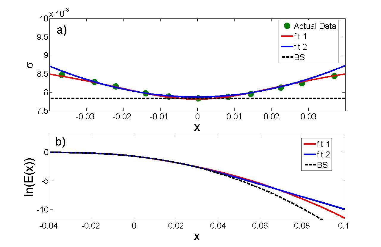
Eq. (13) shows that there is a strong relation between $VS$ and the PDF of financial returns. From another point of view, Eq. (13) should be seen as a warning that shows how similar fits of a VS could imply strong differences in the implied returns of the PDF with obvious consequences, for example, on the risk estimation. If one considers, for example, the two curves (red and blue) in Fig. (2), it is clear that even if the two lines are close to the actual data, the differences in the decay of the two distributions can be relevant with important consequences for the risk estimation procedure.

Figure 2: Comparison of two suitable approximations for the VS (red and blue) (a) and their CCDFs (b). As evident, even if the two curves can be close to the actual data, the differences in the Value at Risk estimation can be relevant. For comparison we also show the case of a completely flat smile (black) and its Gaussian distribution.

One could consider, for example, the estimation of the risk using the standard VAR (value-at-risk) measure Bouchaud , defined as

$$\mathcal{P_{VAR}}=\int_{-\infty}^{-\Lambda_{VAR}}P(x)dx,$$ (16)

where $\Lambda_{VAR}$ represents our estimation of the maximum potential loss with a fixed confidence level given by $\mathcal{P_{VAR}}$ and $P(x)$ is a generic function that represents reuturns PDF. In this paper, we consider $P(x)=P_{\sigma}(x)$ and $\mathcal{P_{VAR}}=1\%$ as a standard value for the confidence level; this means we can expect a loss less than or equal to $\Lambda_{VAR}$ in the $99\%$ of the cases.
For the distributions in Fig. (2), we get $\Lambda_{VAR}^{red}=5.23\%$ and $\Lambda_{VAR}^{blue}=5.06\%$, so the difference in the VAR estimation using the two different fits is about $3.27\%$. To have an idea of the order of magnitude of the error, one should consider that for the flat smile (BS) in the figure, we get $\Lambda_{VAR}^{BS}=4.8\%$ and the difference with the other VAR estimation is about $5\%-8\%$.
From this example it is clear there is some arbitrariness in the fitting parameters of the VS function that can generate significant differences in the description of the implied returns distribution, with important consequences, for example, from the risk estimation point of view. So that the importance of getting a reliable fitting procedure consistent with the theoretical aspects, as already stressed in Ciliberti .
In this framework, we focus our attention on the generalized BS model by considering VS effect and we try to characterize the decay of the tails of the implied distribution of returns as a function of the fitting parameters of the VS, to get a suitable procedure for the smile fitting coherent with the historical observed decay of the actual returns PDFs. As already shown, a suitable characterization of the implied distributions decay can have a fundamental importance, for example, for the risk estimation.

IV Relation between VS and the tails of PDF of financial returns

In this Section, we want to establish a simple relation between the parameters of the fitting function Eq. (9) and the decay of the tails of the implied distribution of returns, Eq. (13). To better understand what we mean for “decay of the tails”, we need to analyze the structure of the Eqs.(9, 13). First of all, it is important to notice that $\sigma(x)$ is a bounded function

$$g\leq\sigma(x)\leq g\chi.$$

The whole process can be seen as a continuous transition from the a minimum value $g$ to a limit value $g\chi$ reached for large enough returns, $x$. From the PDF point of view, we can think of the VS as a continuous transition between two Gaussian distributions with different standard deviations, $g$ and $g\chi$. So, due to our choice of the VS fitting function, we already know that for large $x$ values the tails of the implied distribution behaves as a Gaussian distribution. Nonetheless, there is a region of $x$, namely the region of the transition, not described by a Gaussian, since in this case $\sigma$ is not constant. In Section II we have already discussed the order of magnitude of $x$ for this region: $x\sim\sqrt{n}=2.6g\sqrt{T}$ which corresponds to the tail of the distribution. So, even if we know that for really large $x$ the implied distribution is a Gaussian, the region that can be related to the tails of actual returns distributions is the region of transition and this is the region we are going to study in details.
Looking at a typical implied distribution of returns on a semilog plot it seems reasonable to approximate the region of the transition by a straight line, as shown in Fig. (3).

Figure 3: a) We show the transition region of the VS $\cal{R}$ and b) the exponential decay approximation for the CCDF of returns in the same region.

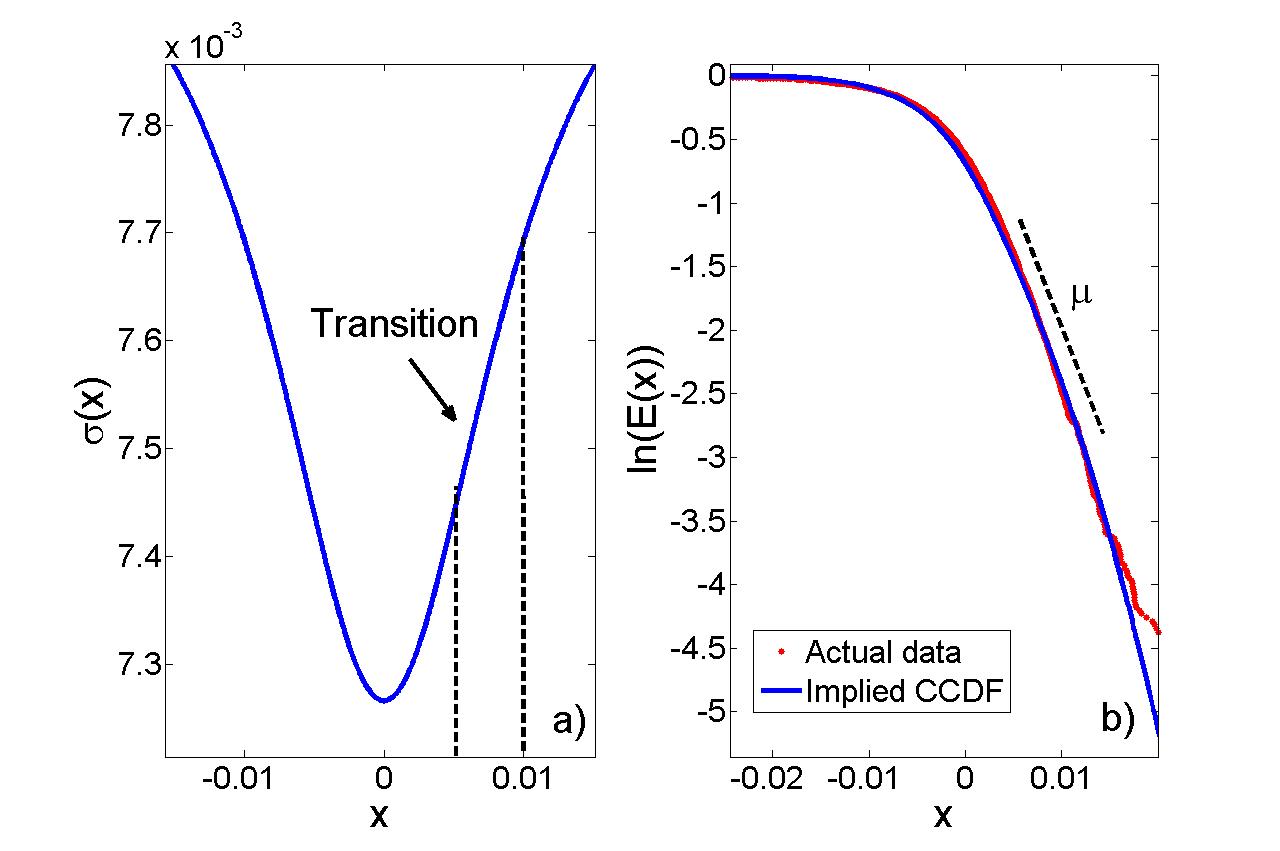
This approximation is equivalent to assume that the tails distributions of financial returns have an exponential decay, $\exp{(-\mu|x|)}$, where $\mu$ is the factor that characterize the tail. This fact finds confirmation in our real data analysis and it is coherent with results shown in Dragulescu .
The main goal of this Section is to establish a relation between the parameter of decay, $\mu$, and the fitting parameters of the smile, $g,\chi,n$. The procedure we consider is straightforward and it is described in the following.
First of all, we fixed the range of the parameters repeating many times the fitting procedure and considering the dataset described in Section II. In Table 2, we show the range of the parameters that we used to perform our simulations (we used the parameter $\rho=n/(g^{2}T)$ instead of $n$ due to the scaling relation Eq. (11)).

	min	max
g	$0.03$	$0.5$
$\rho$	$2.5$	$10$
T (days)	$1$	$1080$
$\chi$	$1.01$	$3$

Table 2: Range of the parameters of the numerical simulations.

Using this range of parameters, we consider the implied CCDF of returns, derived from Eq. (13), and we fit the region of transition considering an exponential decay, $\exp{(-\mu|x|)}$, where $\mu$ is the fitting parameter. In this way we get for every set of the parameters in the Table 2 the corresponding decay parameter, $\mu$. We define the region of transition as ${\cal{R}}=\{x|\sqrt{n}/2\leq x\leq\sqrt{n}\}$; in this way, if $A=g\chi+g$ represents the height of the VS, we are considering the region from the $20\%$ to the $50\%$ of the total height.
Our goal is to find a relation between $\mu$ and the three parameters of the VS. First of all, let us fix $\chi=1$, so that the VS is completely flat. In this case we know that the distribution is Gaussian, $F(x,T,\sigma)=1$ and the parameter $\mu$ should be thought of an approximation of an exponential decay. In this case, $\mu$ can be easily estimated as:

$$\mu=\frac{\Delta y}{\Delta x}=\frac{\ln(\mathcal{P}(\sqrt{n})-\ln(\mathcal{P}(\sqrt{n}/2))}{\sqrt{n}/2},$$ (17)

where $\mathcal{P}$ is the CCDF of $P$ defined in Eq. (13). Performing some calculations we get:

$$\mu_{1}=\frac{2}{g\sqrt{T}}f(\rho),$$ (18)

where, the function $f(\rho)$, is defined by,

$$f(\rho)=\frac{1}{\sqrt{\rho}}\ln\left[\frac{1-\mbox{erf}(\frac{1}{2}\sqrt{\frac{\rho}{2}})}{1-\mbox{erf}(\sqrt{\frac{\rho}{2}})}\right],$$ (19)

and has the following asymptotic expansion:

$$f(\rho)\simeq\left\{\begin{array}[]{rl}\sqrt{\rho}&\mbox{if }\rho\longmapsto+\infty\\ 1/2\sqrt{\pi}&\mbox{if }\rho\longmapsto 0.\end{array}\right.$$ (20)

Let us now discuss the case $\chi\neq 1$: in the light of the adiabatic interpretation presented in Spada , we expect that on increasing $\chi$, the PDF will present, soon or later a minimum. This means that the PDF should be flatter than before, so that $\mu$ should decrease. This is coherent with our physical interpretation of the VS as a small perturbation of a theoretical system represented by a gaussian distribution. Increasing the order of magnitude of the perturbation, here represented by the parameter $\chi$, we get a PDF of returns increasingly different from the gaussian until the adiabatic limit of the perturbation is violated. After that point the system cannot be described by a perturbative approach.

For simplicity, let us assume the simple inverse proportionality:

$$\mu_{\chi}=\displaystyle\frac{\mu_{1}}{\chi}=\frac{2}{\chi g\sqrt{T}}f(\rho).$$ (21)

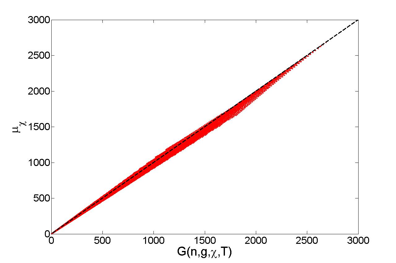
Relation (21) has been checked in Fig. (4) where we plot the real parameter $\mu$ obtained by our simulation vs the parameter $\mu_{\chi}$ given by (21): the agreement is within a $2\%$ of mean squared error.

Figure 4: We show the relation between the decay parameter $\mu$, given by numerical simulation and the estimation given by Eq. (21). As reference, we also show the (dotted) line $\mu=\mu_{\chi}$.

V A new recipe to fit the volatility smile

In this Section we show how to include the information given by the formula (21) on the decay of the CCDF of the financial returns to get a suitable fit of the VS coherent from theoretical point of view. Firstly, to do this we need to analyze what is the ordinary interpretation of the implied volatility of the BS model and its relation with historical volatility. Implied volatility is usually interpreted as the future volatility of the market and represents the traders and practitioners vision. From this point of view historical volatility can be interpreted as a peculiar realization of this vision at some particular time period. So, in general, there will be a mismatch between historical volatility and implied volatility and this fact is reflected on historical and implied PDF of returns. Therefore, to use properly the information on the decay of the historical distribution, we need at first the scaling relation between the volatility and the decay of the distribution. This relation can be estimated from historical series of currencies (AUDUSD, EURCHF, EURGBP, EURJPY, EURUSD, GBPUSD, USDCAD, USDCHF, time period 2001-2010) using the following procedure. We consider different time lag ($T=1,10,100$ days) and build different historical series of returns. We divide each series into subgroups of at least 300 elements and we evaluated the standard deviation of each group. To evaluate the decay we consider the CCDF of returns using the procedure described in Bouchaud and we fit the tail decay using a straight line in a semi log plot. We repeat this procedure for any subgroup and for any currency to make explicit the relation between $\mu_{H}$ and $\sigma_{H}$.

Figure 5: Relation (independent on the time lag $T$) between $\mu_{H}$ and $\sigma_{H}$ considering three different time lag for the returns ($T=1,10,100$). We also show the best linear fit $\ln(\mu_{H})=\ln(\sigma_{H})+ln(C_{1})$, where $C_{1}=1.6\pm 0.5$.

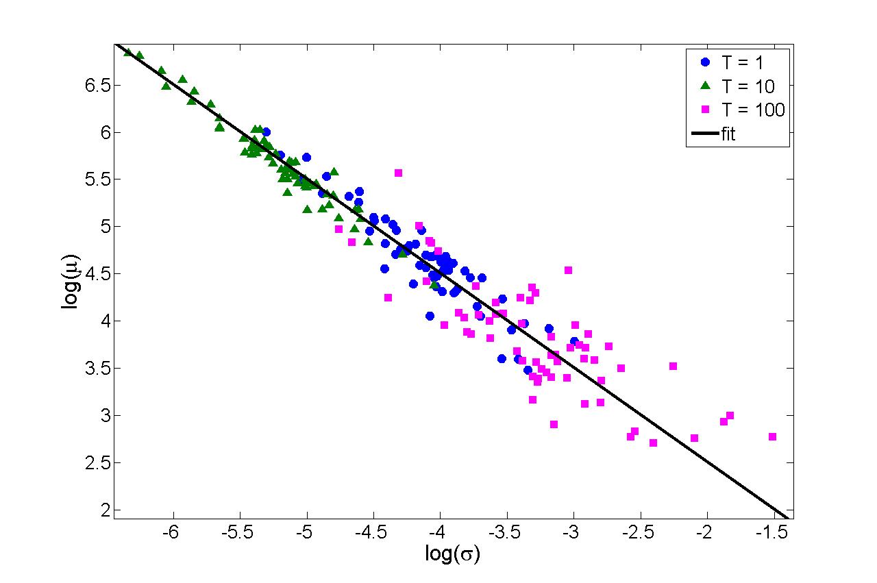
In Fig. (5) we show our results superimposed with a suitable fitting function

$$\sigma_{H}=\frac{C_{1}}{\mu_{H}},$$ (22)

where $C_{1}=1.6\pm 0.5$ is a fitting parameter. Let us observe that this is in quite good agreement with an exponential PDF for returns, since in that case one would have $\sigma_{H}=2/\mu_{H}$.

Eq. (22) makes explicit the relation between $\mu_{H}$ and $\sigma_{H}$ (their product should be a constant $\approx 1.6$) and gives us the opportunity to exploit the information on the historical decay of the PDF of financial returns to get a suitable fit of the VS. The procedure can be summarized as follow:

• Using the historical price series we determine the decay and the standard deviation of the financial returns, respectively: $\mu_{H},\sigma_{H}$.

• Identifying the product $\mu_{H}\sigma_{H}$ with $g\sqrt{T}\mu_{\chi}$ and using our estimation, Eq. (21), we can obtain one of three fitting parameters, e.g. $\chi$, describing the VS, as a function of the other two ($g,n$) :

  $$\chi=\frac{2}{\mu_{H}\sigma_{H}}f(n/g^{2}T).$$ (23)

Following this approach, we reduce the number of free parameters for the smile fitting, fixing implicitly the right decay of the PDF of returns. As already stressed in Section III, the need of getting a suitable fit for the VS coherent also with the theoretical aspects of the model, is really important in many Risk Management activities and could lead to significant differences in risk estimation.

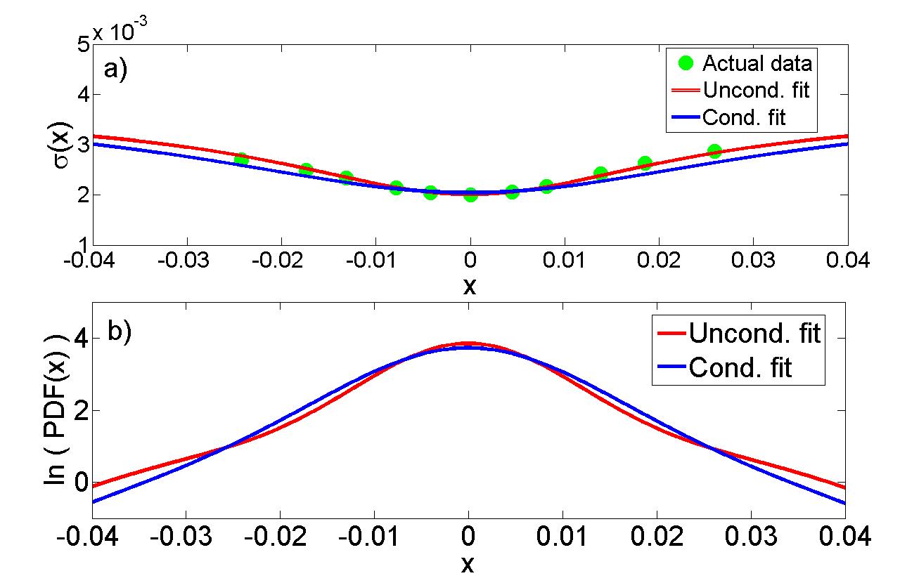
For example in Fig. (6), we compare the PDF of returns obtained by a standard fitting procedure of VS (unconditional fit) with the one obtained following the procedure described before (conditional fit). As evident, even if the two fitting procedures give similar curve for the VS, the effect on the VAR estimation are of the order of $10\%$.

Figure 6: We compare unconditional fit of the VS (a) and the implied PDF (b) for a particular dataset (EURJPY, $T=30$ days, downloaded on 21/10/2009 15:37) with the conditional one.

VI Conclusions

We started from the pricing equation of the Black-Scholes model for an European call and we considered the effect of the VS correction on the implied PDF. Our approach comes from statistical physics and it is related to the adiabatic interpretation in Spada . We showed that similar fits of a VS could imply strong differences on the implied returns PDF with obvious consequences on the risk estimation. To obtain a stronger fitting procedure for the VS that can be compatible with the theoretical aspects of the model we first derived a relation between the exponential decay of the CCDF of returns and the parameters of the fitting function of the smile. Then, we exploit this relation to get a new fitting procedure that can be compatible with the historical data. 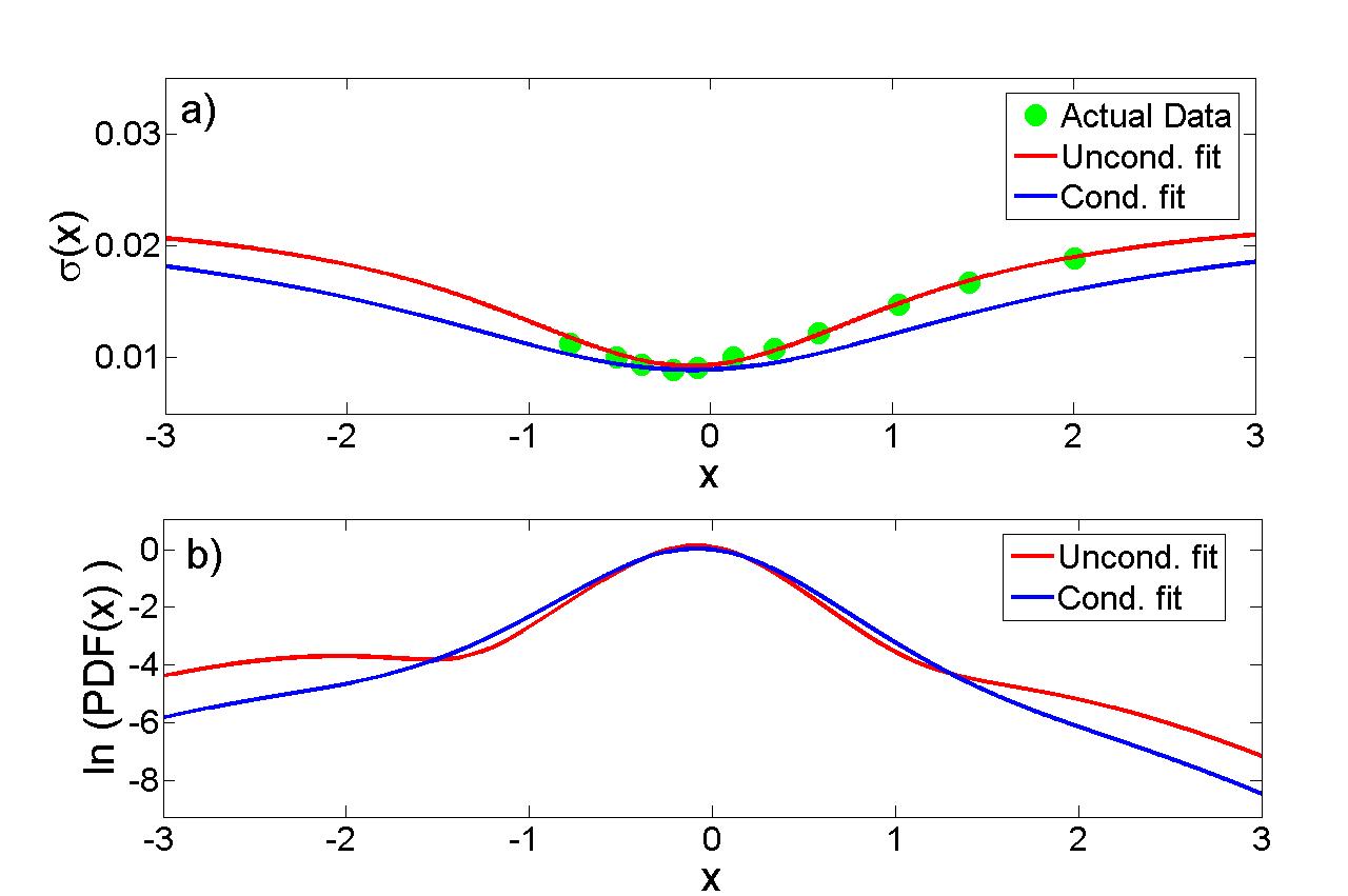An interesting case is shown in Fig. (7) where we compare the PDF of returns obtained by a standard fitting procedure of VS (unconditional fit) with the one obtained following the procedure described before (conditional fit). In this case the time to maturity is large, $T=2520$, so we cannot get $\sigma^{H}$ and $\mu^{H}$ directly from the dataset but we extrapolate their values considering the relation $\mu\propto 1/\sqrt{T}$ and $\sigma\propto\sqrt{T}$. As evident, the unconditional fit generates an implied PDF with a relative minima never observed in actual data Spada , on the contrary the conditional fit generates a PDF more “regular” that seems suitable for the description of actual PDF of returns. The price to pay in order to get a smooth PDF is related to the error for the smile fitting: the horizontal amplitude of the conditional fit is higher than the one required to get a suitable fit. This can be explained assuming that market makers overreact to extreme events when the time to maturity is large, estimating the volatility in a way that is not compatible with historical data. Besides, conditional fit is compatible with the skewness reduction claimed in Ciliberti to get a smile fitting more suitable to the historical data.
In conclusion we provide a new tool for the VS fitting that can be used to get a more coherent estimation of the parameters of fitting function, compatible with historical series and theoretical aspects of the model. A reliable estimate of the implied volatility has application in the risk management activities and in the pricing of exotic derivatives, where, in general, the implied volatility is an input of more complex models.

Figure 7: We compare unconditional fit of the volatility smile (a) and the implied PDF (b) for a particular dataset (EURJPY, $T=2520$ days, downloaded on 21/10/2009 15:37) with the conditional one. To fix the historical decay parameters, $\mu_{H},\sigma_{H}$, we find the values from actual data considering the relation $\mu\propto 1/\sqrt{T}$ (Eq. 22) and the standard scaling $\sigma\propto\sqrt{T}$. As evident, the PDF of conditional procedure does not present spurious minima and gives a distribution suitable to describe actual data.

VII Acknowledgments

The work by GPB was carried out under the auspices of the NNSA of the U. S. DOE at LANL under Contract No. DEAC52-06NA2539.

References

- (1) J. C. Hull, Options, Futures and Other Derivatives, Prentice Hall, Upper Saddle Rivel, New Jersey (2003).
- (2) P. Willmott, Derivatives, John Wiley and Sons, Chinchester, New York, Weinheim, Brisbane, Singapore, Toronto (1998).
- (3) F. Black, M. Scholes, The Pricing of Options and Corporate Liabilities, Journal of Political Economy 81, 637-654 (1973).
- (4) The behavior of the Wiener process can be described on the finite time-interval, , as ,where the random variable, , has the distribution function: .
- (5) J. -P. Bouchaud, M. Potter, Theory of Financial Risk - From Statistical Physics to Risk Management, University Press, Cambridge (2000).
- (6) S. L. Heston, A Closed-Form Solution for Options with Stochastic Volatility with Applications to Bond and Currency Options, The Review of Financial Studies, 6, 2, 327-343 (1993).
- (7) P. Hagan, D. Kumar, A. Lesniewski and D. Woodward, Managing Smile Risk, Wilmott Magazine, 1, 84-108 (2002).
- (8) L. Spadafora, G.B. Berman, F. Borgonovi, Adiabaticity Conditions for Volatility Smile in Black-Scholes Pricing Model in press EPJB, arXiv:/1003.3316v2 (2010).
- (9) L. D. Landau, E. M. Lifshitz, Mechanics, Butterworth-Heinenann, Oxford, UK (2000).
- (10) G. Brown, C. Randall, If the Skew Fits, Risk Magazine 12 (4), 62-65 (1999).
- (11) R. Tompkins, Implied Volatility Surfaces: Uncovering the Regularities for Options on Financial Futures, The European Journal of Finance 7, 198-230 (2001).
- (12) K. Toft, B. Prucyk, Options on Leveraged Equity: Theory and Empirical Tests, Journal of Finance 52(3), 1151-1180 (1997).
- (13) J. Campa, K. Chang, R. Reider, Implied Exchange Rate Distributions: Evidence from OTC Option Markets, Journal of International Money and Finance 17 (1), 117-160 (1998).
- (14) V. F. Pisarenko, D. Sornette, New Statistic for Financial Returns Distributions: Power-Law or Exponential?, Physica A 366, 387-400 (2006).
- (15) P. Gopikrishnan, M. Meyer, L. A. N. Amaral, H. E. Stanley, Inverse Cubic Law for the Distribution of Stock Price Variations, European Physical Journal B 3 (2), 139-140 (1998).
- (16) U. Kirchner, Market Implied Probability Distributions and Bayesian Skew Estimation, arXiv:/0911.0805 (2009).
- (17) A. M. Malz, Option-Implied Probability Distribution and Currency Excess Returns, FRB of New York Staff Report 32 (1997).
- (18) S. Ciliberti, J. -P. Bouchaud, M. Potter, Smile dynamics - a theory of the implied leverage effect, arXiv:/0809.3375v1 (2008).
- (19) A. A. Dragulesco and V. M. Yakovenko, Probability distribution of returns in the Heston model with stochastic volatility, Quantitative Finance, 2, 443-453 (2002).