Cauchy problem for multiscale conservation laws:
Application to structured cell populations
††thanks: This work was supported by the large scale INRIA project REGATE (REgulation of
the GonAdoTropE axis).
Abstract
In this paper, we study a vector conservation law that models the growth and selection of ovarian follicles. During each ovarian cycle, only a definite number of follicles ovulate, while the others undergo a degeneration process called atresia. This work is motivated by a multiscale mathematical model starting on the cellular scale, where ovulation or atresia result from a hormonally controlled selection process. A two-dimensional conservation law describes the age and maturity structuration of the follicular cell populations. The densities intersect through a coupled hyperbolic system between different follicles and cell phases, which results in a vector conservation law and coupling boundary conditions. The maturity velocity functions possess both a local and nonlocal character. We prove the existence and uniqueness of the weak solution to the Cauchy problem with bounded initial and boundary data.
Keywords: conservation laws, nonlocal velocity, multiscale, biomathematics
2000 MR Subject Classification: 35L65, 92D25, 92B05.
1 Introduction
In this paper, we study the following vector conservation law
| (1.1) |
where , , and
Here and are positive constants, , , , and all belong to , with the local control and the global control, where and are continuous differentiable, i.e., and . For instance, the specific case that motivated our work is presented in Appendix 6.1. The function is the maturity on the follicular scale given by
and
is the global maturity on the ovarian scale. The parameters and are positive constants with .
This work is motivated by problems of cell dynamics arising in the control of the development of ovarian follicles. Ovarian follicles are spheroidal structures sheltering the maturing oocyte. During each ovarian cycle, numerous follicles are in competition for their survival. However, only very few follicles reach an ovulatory size, most of them undergo a degeneration process, known as atresia (see for instance [12]). A mathematical model, proposed by F. Clément [5] using both multi-scale modeling and control theory concepts, describes the follicle selection process. For each follicle, the cell population dynamics is ruled by a conservation law, which describes the changes in cell age and maturity. Two acting controls, and (see [1] and also Appendix 6.1), are distinguished. The global control results from the ovarian feedback onto the pituitary gland and impacts the secretion of the follicle stimulating hormone (FSH). The feedback is responsible for reducing FSH release, leading to the degeneration of all but those follicles selected for ovulation. The local control , specific to each follicle, accounts for the modulation in FSH bioavailability related to follicular vascularization. In addition, the status of cells are characterized by three phases. Phase 1 and 2 correspond to the proliferation phases, and Phase 3 corresponds to the differentiation phase (see Fig 1). In Appendix 6.2, we have reformulated the original model to a new system (1.1), where the unknowns are all defined on the same domain , so that it can be treated as a general model for multiscale structured cell populations (see Appendix 6.2 for the relation between the original notations and the new notations).
The initial conditions are given by
| (1.2) | ||||
We use the simplified notations , , and in the whole paper.
The boundary conditions at are given by
| (1.3) |
The boundary conditions at are given by
| (1.4) |
The boundary conditions at are given by
| (1.5) |
.
The well-posedness problems of the hyperbolic conservation laws have been widely studied for a long time. We refer to the works [7, 8, 9, 15, 16] (and the references therein) in the content of weak solutions to systems in conservation laws, and [13, 14] in the content of classical solutions to general quasi-linear hyperbolic systems. In this paper, we perform the mathematical analysis of this system: we prove the existence, uniqueness and regularity of the weak solution to the Cauchy problem defined by (1.1)-(1.5) with initial and boundary data in . The main difficulty tackled with in this paper comes from the nonlocal velocity, the coupling between boundary conditions and the coupling between different follicles in the model. Additionally, we have to deal with loss terms, and the problem is a 2 - space dimension one.
In the related works that have considered nonlocal velocity problems [3, 4], the problems are only 1 - space dimension and do not have source terms. The velocities there are always positive, while in our case, the velocities we considered in this paper change sign in Phase 3. In another related work [10], which was also motivated by [5], the author has performed a mathematical analysis on this kind of model. He has reduced the model to a 1-space dimension mass-maturity dynamical system of coupled Ordinary Differential Equations, basing on the asymptotic properties of the original law. Once reduced, the model is amenable to analysis by bifurcation theory, that allows one to predict the issue of the selection for one specific follicle amongst the whole population. And he gave some assumptions on velocities according to biological observations. In another work [11], the author also studied the well-poseness of the model, he proved the existence of a measure valued solution without proving the uniqueness of the solution, and he gave the behavior of the solution to the main equation along its characteristics. An associated reachability problem has been tackled in [6], which described the set of microscopic initial conditions leading to the macroscopic phenomenon of either ovulation or atresia in the framework of backwards reachable sets theory. The authors also performed some mathematical analysis on well-poseness of this model in a simplified open loop like case, there the authors assumed that the local control and the global control are given functions of time . While in this paper, we consider the close/open loop case.
This paper is organized as follows. In Section 2 we first give the main results. In Section 3 after giving some basic notations, we prove that the vector maturity exists as a fixed point of a map from continuous function space, and then we construct a local weak solution to the Cauchy problem defined by (1.1)-(1.5). In Section 4 we prove the uniqueness of the weak solution. Finally in Section 5 we prove the existence of a global solution. In complement, we introduce in Appendix 6.1 the original mathematical model proposed by F. Clément [5]. In Appendix 6.2 we reformulate this model to the new system (1.1) and we give the equivalence between the original notations and the new notations. In Appendix 6.3 we give a basic lemma that is used to prove the existence and uniqueness of the weak solution.
2 Main results
We recall from [2, Section 2.1], the usual definition of a weak solution to the Cauchy problem defined by (1.1)-(1.5).
Definition 2.1.
With the definition, we have the main result
Theorem 2.1.
Let , be given. Let us further assume that
The sketch of the proof of Theorem 2.1 consists in first proving that the maturity exists as a fixed point of the map (see Section 3.1), and then in constructing a (unique) local solution (see Section 3.2 and Section 4), before finally proving the existence of a global solution to the Cauchy problem defined by (1.1)-(1.5) (see Section 5).
3 Fixed point argument and construction of a local solution to the Cauchy problem
In this section, we first derive the contraction mapping function . Given the existence of fixed point to this contraction mapping function, we can then construct a local solution to the Cauchy problem defined by (1.1)-(1.5).
3.1 Fixed point argument
First we introduce some notations. Let us define:
| (3.1) | ||||
| (3.2) | ||||
| (3.3) | ||||
For any , let
where the constant is given by (3.1).
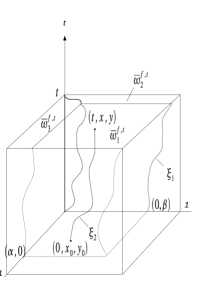
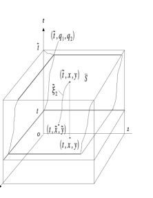
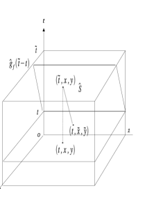
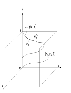
In order to derive the expression of the contraction mapping function , we solve the corresponding linear Cauchy problem (1.1)-(1.5) with given . For any fixed and , we trace back the density function at time along the characteristics to the initial and boundary data, hence we divide the plane time into several parts. For Phase 1, the velocities are always positive, we introduce three subsets , and of (see Fig 2 (a))
Here (see Fig 2 (a))satisfies
| (3.4) |
with defined by .
If , we trace back the density function at time along the characteristics to the initial data. Otherwise, we trace back the density function at time along the characteristics to the boundary data. For any fixed and , let us define characteristics (see Fig 2), which will be used to construct the contraction mapping function.
In the whole paper, we denote by the points on the bottom face , the points on the left face , the points on the right face , the points on the back face and the points on the front face .
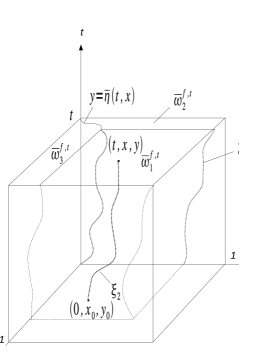
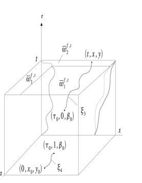
For any fixed , we define characteristic by (see Fig 2 (a))
If (see Fig 2 (a)), we define characteristic by
One has . Let us define
| (3.5) |
If (see Fig 2 (b)), we define characteristic by
There exists a unique such that , so that we can define
| (3.6) |
According to the coupled boundary between Phase 1 at and Phase 2 at , for any fixed , we define characteristic by (see Fig 2 (b))
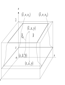
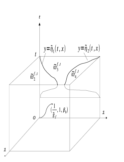
For Phase 3, due to the fact that velocities change sign in Phase 3, we divide the plane at time into four subsets , , and of (see Fig 3 (a))
Here and (see Fig 3 (a)) satisfy
If , we trace back the density function at time along the characteristics to the initial data. Otherwise, we trace back the density function at time along the characteristics to the boundary data. For any fixed and , let us define characteristics (see Fig 3), which will be used to construct the contraction mapping function.
If (see Fig 3 (a)), we define characteristic by
One has . Let us define
| (3.7) |
If (see Fig 3 (a)), we define characteristic by
There exists a unique such that , so that we can define
| (3.8) |
For any fixed cell cycle , according to the coupled boundary between Phase 1 and Phase 3 (corresponding to at and at ), we separate the right face of Phase 1 into two parts. For , we define characteristic passing through the right face intersects with the bottom face at (see Fig 3 (b)). For , we define characteristic passing through the right face intersects with the back face, and then back to the bottom face at of the cell cycle in Phase 2 (see Fig 3 (b)). Hence, for any fixed , we define by
and by
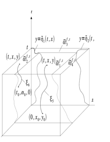
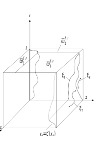
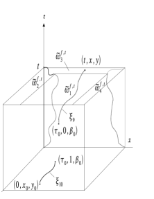
If (see Fig 3 (c)), we define characteristic by
There exists a unique such that , so that we can define
| (3.9) |
According to the coupled boundary between two consecutive cell cycles (corresponding to at and at ) , for any fixed , we define by (see Fig 3 (c))
With all of the above defined characteristics and noting Lemma 6.1 in Appendix 6.3, we are now able to define a map for all with
| (3.10) | ||||
Here can also be determined by , is defined by , is defined by , and is defined by . In (3.10), (see Fig 3 (b)), where satisfies
with defined by .
Next we prove the following fixed point theorem.
Lemma 3.1.
If is small enough, is a contraction mapping on with respect to the norm.
Proof:.
It is easy to check that maps into itself if
| (3.11) |
where is defined by (3.2). Let , , and , . In order to estimate , we first estimate the norms separately. Observing the definition (3.10) of , it is sufficient to estimate , where
| (3.12) |
Here denotes various constants, represents or , and . We have
hence
| (3.13) |
By (3.13), we have
| (3.14) | ||||
Similarly, we have
| (3.15) |
where represents or , and
| (3.16) |
By (3.13)-(3.16) and the definition (3.10) of , we have
| (3.17) |
The expressions of and are given by (6.30) in Appendix 6.3. They depend on and . Thus we have
| (3.18) | ||||
We finally get
| (3.19) |
Hence we can choose small enough (depending on ) so that
| (3.20) |
∎
By Lemma 3.1 and the contraction mapping principle, there exists a unique fixed point in .
3.2 Construction of a local solution to the Cauchy problem
Now we show how the fixed point allows to find a solution to Cauchy problem (1.1)-(1.5) for . Let us recall the definition of three subsets , and of , the definition of the characteristics and also the definition (3.5) of and (3.6) of . For , we define by
| (3.21) |
For , we define by
| (3.22) |
Since the dynamic in Phase 2 amounts to pure transport equations, we define , by
| (3.23) |
Let us recall the definition of the four subsets , , and of , the definition of the characteristics and also the definition (3.7) of , (3.8) of and (3.9) of . For , we define by
| (3.24) |
For , we define by
| (3.25) |
Next we prove that the vector function defined by (3.21)-(3.25) is a weak solution to Cauchy problem (1.1)-(1.5) for . To that end, we first prove that defined by (3.21)-(3.25) satisfies equality (2.5) of Definition 2.1, then we prove that . Let . For any vector function , such that (2.1)-(2.4) hold, by definition (3.21)-(3.25) of , we have
| (3.26) |
In (3.26),
Let us consider the first term as an instance. By the change of variable and noting (6.21) of Lemma 6.1 in Appendix 6.3, we have
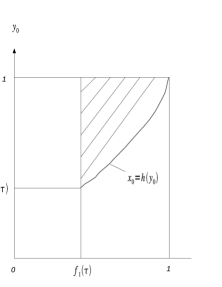
where (see Fig 4 (a) and (b))
| (3.27) |
Clearly, is a function of , suppose that . After changing the order of integration, can be rewritten as
Changing the order of integration again (see Fig 4 (c)), we obtain
| (3.28) |
By (3.28) and noting that , we get
| (3.29) |
Similar to , we can prove that
| (3.30) | |||
| (3.31) | |||
| (3.32) | |||
| (3.33) | |||
| (3.34) | |||
| (3.35) |
By (3.29)-(3.35), we have proven that the vector function defined by (3.21)-(3.25) satisfies (2.5). Next we prove that . Moreover, we can prove that even belongs to , for all .
Proof:.
From the definition (3.21)-(3.25) of , we get easily that . Next we prove that the vector function belongs to for all , i.e., for every with (the case that can be treated similarly), we need to prove
In order to do that, we estimate , and separately.
Suppose that the characteristic passing through intersects time plane at (see Fig 5 (a)), we have
where satisfies
We get easily that
| (3.36) |
Here and hereafter in this section, we denote by various constants which do not depend on , , or . Let (see Fig 5 (a)), following our method to construct the solution , when , we have
Here denotes the characteristic passing through that intersects time plane at . Hence is defined by
We have
| (3.37) |
Since , for every , there exists such that for every , there exists satisfying
| (3.38) |
Here and hereafter in this section, we denote by various constants that may depend on (the index of the corresponding approximating sequences , and ) but are independent of .
Thus, we have
| (3.39) |
| (3.40) |
Noting (3.36), we have
| (3.41) |
Combining (3.40) with (3.41), we obtain
| (3.42) |
Next we estimate . For Phase 2, the characteristic passing through intersects time plane at . Let (see Fig 5 (b)), when , we have
Since , for every , there exists such that for every , there exists satisfying
| (3.43) |
Similar to (3.40), we can prove that
| (3.44) |
It is easy to check that
| (3.45) |
Combining (3.44) with (3.45), we get
| (3.46) |
Finally, we estimate . Suppose that the characteristic passing through intersects time plane at , and the characteristic passing through intersects time plane at (see Fig 5 (c)). Similar to (3.36), we can prove that
| (3.47) |
Let (see Fig 5 (c)), when , we have
Here denotes the characteristic passing through that intersects time plane at . Similar to (3.37), we can prove that
Since , for every , there exists such that for every , there exists satisfying
| (3.48) |
Similar to (3.40), we can prove that
| (3.49) |
Noting (3.47), we have
| (3.50) |
Combining (3.49) with (3.50), we get
| (3.51) |
Therefore letting be large enough and then be small enough, the right hand side of (3.42), (3.46) and (3.51) can be arbitrarily small. Above all, we prove that the vector function belongs to for all . ∎
4 Uniqueness of the solution
In this section, we prove the uniqueness of the solution.
Proof:.
Assume that is a weak solution to Cauchy problem (1.1)-(1.5). Similar to Lemma 2.2 in [3, Section 2.2], we can prove that for any fixed and any with
one has
| (4.1) | ||||
In (4.1), the velocity matrices , and are defined the same way as , and but with and instead of and , where
and . Let , and choose the test function as the solution to the following backward linear Cauchy problem
| (4.2) |
For any fixed , we introduce three new subsets , and of
Here satisfies
with defined by .
For any fixed and . If , we define by
Let us then define
| (4.3) |
If , we define by
There exists a unique such that , so that we can define
| (4.4) |
By (4.1) and (4.2), we obtain that
| (4.5) | ||||
Let us recall the definition of the characteristic and also the definition (4.3) of . By solving the backward linear Cauchy problem (4.2) and noting (6.21) of Lemma 6.1 in Appendix 6.3, we have
| (4.6) |
As for the last term of (4.5), by solving the backward linear Cauchy problem (4.2), we have
Since and are both arbitrary, we obtain in that for
| (4.7) |
Let us recall the definition of the characteristic and also the definition (4.4) of . By solving the backward linear Cauchy problem (4.2), noting (4.7) and (6.22) of Lemma 6.1 in Appendix 6.3, we have
Since and are both arbitrary, we obtain in that for
| (4.8) |
For , we have
| (4.9) |
For any fixed , we introduce four new subsets , , and of
Here and satisfy
For any fixed and . If , we define by
Let us then define . By solving the backward linear Cauchy problem (4.2) and noting (6.24) of Lemma 6.1 in Appendix 6.3, the last term of (4) can be rewritten as
If , we define by
There exists a unique such that , so that we can define . By solving the backward linear Cauchy problem (4.2), and noting (6.25) of Lemma 6.1 in Appendix 6.3, we have
If , we define by
There exists a unique such that , so that we can define . By solving the backward linear Cauchy problem (4.2) and noting (6.28) of Lemma 6.1 in Appendix 6.3, we have
Since and are both arbitrary, we obtain in that for
| (4.10) |
For , we get
| (4.15) |
By (3.11), we claim that and satisfies the same contraction mapping function . Since is the unique fixed point of in , therefore we have . Consequently, we have , and , so that , , , and . Finally, by comparing the definition (4.7)-(4.15) of with the definition (3.21)-(3.25) of , we obtain . This gives us the uniqueness of the weak solution for small time. ∎
5 Proof of the existence of a global solution to the Cauchy problem
Let us now prove the existence of global solution to Cauchy problem (1.1)-(1.5). Noting the definition (3.10) of and the definition (3.21)-(3.25) of the local solution , it is easy to check that the following two estimates hold for all
| (5.1) |
| (5.2) |
where is defined by (3.1), is defined by (3.2) and is defined by (3.3). In order to obtain a global solution, we suppose that we have solved Cauchy problem (1.1)-(1.5) up to the moment with the weak solution . It follows from our way to construct the weak solution, we know that for any , the weak solution is given by for
| (5.3) |
For
| (5.4) |
For
| (5.5) |
| (5.6) |
For
| (5.7) |
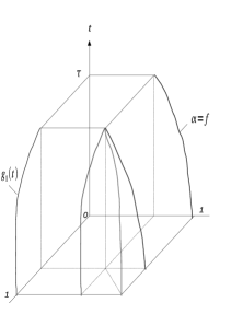
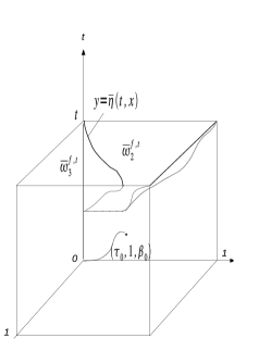
As time increases, for each cell cycle in Phase 1, the characteristic passing through the origin may have two possible cases. It may either intersect with the front face (see Fig 6 (a)) or intersect with the right face (see Fig 6 (b)). For each cell cycle in Phase 3, the characteristic passing through the origin will definitely intersect with the front face due to the fact that (see Fig 6 (c)). We get in any case that
We can prove that estimate (5.1) holds for every by tracing back , and along the characteristics to the initial data at most times. Moreover, noting the definition (5.3)-(5.7) of the global solution, it is easy to check that the uniform a priori estimate (5.2) holds for every . Hence we can choose independent of . Applying Lemma 3.2 and Lemma 4.1 again, the weak solution is extended to the time interval . Step by step, we finally obtain a unique global weak solution . This finishes the proof of the existence of a global solution to Cauchy problem (1.1)-(1.5).
6 Appendix
6.1 Introduction of the model
In this section, we first recall the systems of equations describing the dynamics of the cell density of a follicle in the model of F. Clément [1, 5, 6]. The cell population in a follicle is represented by cell density functions defined on each cellular phase with age and maturity , which satisfy the following conservation laws
| (6.1) |
Here , and is the number of consecutive cell cycles (see Fig 7).
Define the maturity operator as
| (6.2) |
Then
| (6.3) |
is the global follicular maturity on the follicular scale, while
| (6.4) |
is the global maturity on the ovarian scale.
The velocity and source terms are all smooth functions of and , where is the local control and is the global control. In this paper, we consider close/open loop problem, that is to say and are functions of and . As an instance of close loop problem, the velocity and source terms are given by the following expressions in [1] (all parameters are positive constants)
The initial conditions are given as follows
| (6.5) |
The boundary conditions are given as follows
For sake of simplicity, we denote by in the whole paper the difference between the maximum of the maturity in Phase 1 and the maximum of the maturity in Phase 3.
6.2 Mathematical reformulation
In this section, we perform a mathematical reformulation of the original model introduced in Appendix 6.1. Notice that in system (6.1), all the unknowns are defined on different domains, so that one has to solve the equations successively. Here we transform system (6.1) into a regular one where the unknowns are defined on the same domain . We denote by the density functions and by and the age and maturity velocities for Phase 1; the density functions and the age velocities for Phase 2; the density functions and , the age and maturity velocities for Phase 3.
Let
| (6.6) |
where
| (6.7) |
so that we get , and
| (6.8) |
with
| (6.9) |
Let
| (6.10) |
where
| (6.11) |
So that we get , and
| (6.12) |
Let
| (6.13) |
where
| (6.14) |
so that we get , and
| (6.15) |
with
| (6.16) |
Accordingly, let us denote the initial conditions (6.5) with new notations by
| (6.17) |
where
| (6.18) |
Let , we have
| (6.19) |
where
From the original expression of (see Appendix 6.1), let us define
It is easy to see that is an increasing function of , and
Hence, when , we have , moreover
Furthermore, under the assumption that the local control satisfies , and
From the fact that in Phase 1, and in Phase 3, we have
Corresponding to the new notations, we have assumptions
| (6.20) |
Since
We have
6.3 Basic lemmas and some notations
The following lemma is used to prove the existence of the weak solution to Cauchy problem (1.1)-(1.5), when we derive the contraction mapping function , change variables in certain integrals (see Section 3) and prove the uniqueness of the solution (see Section 4).
Lemma 6.1.
The characteristic passing through intersects the bottom face at . We have
| (6.21) |
The characteristic passing through intersects the back face at . We have
| (6.22) |
The characteristic passing through intersects the bottom face at . We have
| (6.23) |
The characteristic passing through intersects the bottom face at . We have
| (6.24) |
The characteristic passing through intersects the left face at . We have
| (6.25) |
The characteristic passing through intersects the bottom face at . We have
| (6.26) |
The characteristic passing though intersects the back face at . We have
| (6.27) |
The characteristic passing through intersects the back face at . We have
| (6.28) |
The characteristic passing through intersects the bottom face at . We have
| (6.29) |
The proof of this lemma is trivial, and can be found in [14] of 1-space dimension case, we omit here.
The expressions of contraction mapping coefficients and are as following
| (6.30) | ||||
Acknowledgements
The author would like to thank the professors Frédérique Clément, Jean-Michel Coron and Zhiqiang Wang for their interesting comments and many valuable suggestions on this work.
References
- [1] F. Clément. Multiscale modelling of endocrine systems: new insight on the gonadotrope axis. ESAIM: proceedings, 27 :209-226, 2009.
- [2] J.-M. Coron, Control and nonlinearity, Mathematical Surveys and Monographs 136, American Mathematical Society, Providence, RI, 2007.
- [3] J.-M. Coron, M. Kawski, and Z. Wang. Analysis of a conservation law modeling a highly re-entrant manufacturing system, preprint, arXiv:0907.1274v1.
- [4] P. Shang and Z. Wang. Analysis and control of a scalar conservation law modeling a highly re-entrant manufacturing system, preprint, arXiv:1003.4411v1.
- [5] N. Echenim, D. Monniaux, M. Sorine, and F. Clément. Multi-scale modeling of the follicle selection process in the ovary. Math. Biosci., 198 :57–79, 2005.
- [6] N. Echenim, F. Clément, and M. Sorine. Multi-scale modeling of follicular ovulation as a reachability problem. Multiscale Model. Simul., 6 :895–912, 2007.
- [7] S. Bianchini and A. Bressan, Vanishing viscosity solutions of nonlinear hyperbolic systems, Ann. of Math., (2) 161 (2005), pp. 223–342.
- [8] A. Bressan, Hyperbolic systems of conservation laws. The one dimensional Cauchy problem, Oxford University Press, Oxford, 2000.
- [9] S. N. Kružkov. First order quasilinear equations in several independent variables. Sb. Math., 10(2) :217-243, 1970.
- [10] P. Michel. Multiscale modeling of follicular ovulation as a mass and maturity dynamical system, 2009.
- [11] P. Michel. Existence of measure solution to a renewal equation, 2009.
- [12] EA. McGee and AJ. Hsueh. Initial and cyclic recruitment of ovarian follicles. Endocrine Reviews, 21(2) :200-214, 2009.
- [13] T.-T. Li, Global classical solutions for quasilinear hyperbolic systems, Research in Applied Mathematics 32, John Wiley & Sons, Chichester, 1994.
- [14] T.-T. Li and W. C. Yu, Boundary value problems for quasilinear hyperbolic systems, Duke University Mathematics Series V, Duke University, Mathematics Department, Durham, NC, 1985.
- [15] T.-P. Liu and T. Yang, Well-posedness theory for hyperbolic conservation laws, Comm. Pure Appl. Math. 52 (1999), no. 12, pp. 1553–1586.
- [16] A. Poretta and J. Vovelle. solutions to first order hyperbolic equations in bounded domains, Communications in Partial Differential Equations, Volume 28, 381-408, 2003.