Statistical Properties of Cross-Correlation in the Korean Stock Market

Abstract

We investigate the statistical properties of the correlation matrix between individual stocks traded in the Korean stock market using the random matrix theory (RMT) and observe how these affect the portfolio weights in the Markowitz portfolio theory. We find that the distribution of the correlation matrix is positively skewed and changes over time. We find that the eigenvalue distribution of original correlation matrix deviates from the eigenvalues predicted by the RMT, and the largest eigenvalue is 52 times larger than the maximum value among the eigenvalues predicted by the RMT. The $\beta_{473}$ coefficient, which reflect the largest eigenvalue property, is 0.8, while one of the eigenvalues in the RMT is approximately zero. Notably, we show that the entropy function $E(\sigma)$ with the portfolio risk $\sigma$ for the original and filtered correlation matrices are consistent with a power-law function, $E(\sigma)\sim\sigma^{-\gamma}$, with the exponent $\gamma\sim 2.92$ and those for Asian currency crisis decreases significantly.

I Introduction

Financial markets have been known as representative complex systems, which are organized by various unexpected phenomenon according to non-trivial interactions among heterogeneous agents Thomas Lux . The study of complex economic systems is not easy because we do not know the control parameters that govern economic systems and can not easily apply the parameters we do know to economic systems. However, much research has been conducted to understand the statistical properties of financial time series Mantegna(a) ; Oh . In particular, the analysis of financial data by various methods developed in statistical physics has become a very interesting research area for physicists and economists Mantegna&Bouchaud . There is practical Elton ; Okhrin ; Sornette as well as scientifically important value in analyzing the correlation coefficient between stock return time series because this contains a significant amout of information on the nonlinear interactions in the financial market and is a parameter in terms of the Markowitz portfolio theory. The correlation matrix between stocks, which has unexpected properties due to complex behaviors, such as temporal non-equilibrium, mispricing, bubbles, market crashes and so on, is an important parameter to understand the interactions in the financial market Noh . To analyze the correlation matrix, previous studies presented various statistical methods, such as principal component analysis (PCA) PCA , singular value decomposition (SVD) SVD and factor analysis (FA) FA . Here, to analyze the actual correlation matrix, we employ the random matrix theory (RMT), which was introduced by Wigner, Dyson and Metha MehtaB ; Wigner ; Dyson ; Mehta . It can explain the statistical properties of energy levels in complex nuclei well. The RMT method is a useful method for eliminating the randomness in the actual correlation matrix Guhr1 ; Sengupta ; Seba ; Utsugi ; Guhr2 ; Shari . Recently, Laloux et al (1999) Laloux and Plerou et al (1999) Plerou1 analyzed the correlation matrix of financial time series by the RMT method. The authors found that 94% of the eigenvalues of correlation matrix can be predicted by the RMT, while the other 6% of the eigenvalues deviated from the RMT. In addition, Plerou et al (2002) Plerou2 applied the RMT method to a United States stock market and observed that the correlation matrix of stock markets consist of random and non-random parts, which have a useful information in the financial market. The eigenvector deviations from the RMT show a very stable state over a whole period. We investigate the various statistical properties of the correlation matrix of 473 daily stock return time series traded in the Korean stock market from 1 January 1993 to 31 May 2003. We find that the distribution of the correlation matrix is positively skewed and changes over the whole time. Using the RMT method, we show that the correlation matrix contains meaningful information as well as random property. Notably, we show that for both the original, $C_{original}$, and filtered correlation, $C_{filter}$, matrices the entropy function, $E(\sigma)$, with the portfolio risk, $\sigma$, is consistent with a power-law function, $E(\sigma)\sim\sigma^{-\gamma}$, with an exponent $\gamma\sim 2.92$. In the following section, we describe the data and methods used in this paper. In Section 3, we present the verification results. Finally, we end with a conclusion.

II Data and Method

In this paper, we investigate the statistical properties of the correlation matrix of the 473 daily stock returns traded on the Korean stock market from 3 January 1993 to 31 May 2003. The data obtained from the Korea Stock Exchanges cover 2845 days. To understand the non-trivial interactions, we calculated the correlation matrix between stocks for the whole period as well as sub-periods by shifting 21 days with 250 data points. We propose a verification process to analyze the statistical properties of the correlation matrix between stock returns. First, we estimated the statistical properties of the correlation matrices using the RMT method. Second, we calculate the entropy of the portfolio weights using the Markowitz portfolio theory. Before demonstrating the verification process, we introduces the RMT, which was proposed by Wigner, Dyson, and Metha, et al. and Markowitz portfolio theory (MPT) Markowitz introduced by Markowitz in 1952. We created $N$ (number of company) data sets with $L$ data points following $iid(0,1)$. Let the created data be denoted by the symbol $G$. Here, the $G$ is a matrix ($N\times L$) with the random elements and the correlation matrix is defined by

$$C_{random}=\frac{1}{L}GG^{T},$$ (1)

where $G^{T}$ is the transpose of $G$, and the correlation between elements is approximately zero. If $N\to\infty$ and $L\to\infty$, the eigenvalue spectrum of RMT is calculated by using

$$P_{random}(\lambda)=\frac{Q}{2\pi}\frac{\sqrt{(\lambda_{+}-\lambda)(\lambda-\lambda_{-})}}{\lambda},$$ (2)

where the eigenvalues $\lambda$ lie within $\lambda_{-}\leq\lambda\leq\lambda_{+}$, $Q\equiv\frac{L}{N}$, and the maximum and minimum eigenvalue of RMT, $C_{random}$, are given by

$$\lambda\pm\equiv 1+\frac{1}{Q}\pm 2\sqrt{\frac{1}{Q}}.$$ (3)

If $L$ and $N$ have a limitable length, then the eigenvalue spectrum shows gradual decrease from the theoretical values of the largest eigenvalue predicted by the RMT.

We next explain the MPT to select the optimal portfolio sets among all stocks. The MPT method introduced by Markowitz in 1952 is generically known as the mean-variance theory. The purpose of MPT is to minimize the portfolio risk in a given portfolio return, which can be quantified by the variance and defined as follows.

$$\Omega=\sum_{i=1}^{N}\sum_{j=1}^{N}\omega_{i}\omega_{j}C_{ij}\sigma_{i}\sigma_{j},$$ (4)

where $\omega_{i}$ is the portfolio weight of stock $i$, which can be calculated using two Lagrange multipliers, $\sigma_{i}$ is the standard deviation of stock $i$, and $C_{ij}$ is the correlation coefficient between stock $i$ and stock $j$. In this work, we use the no short-selling constraint for portfolio weights Mantegna&Bouchaud , i.e. we assume that all the weights are non negative numbers ($\omega_{i}>0$, $\forall$ i=1,$\dots$,N). We also normalize portfolio weights in such a way that $\sum_{i=1}^{N}\omega_{i}=1$. The portfolio return, $\mu$, also is calculated by

$$\mu=\sum_{i=1}^{N}\omega_{i}\mu_{i},$$ (5)

where $\mu_{i}$ is the mean value of stock $i$. We next considered the portfolio weights because these could determine the portfolio efficiency frontier lines. We used Shannon’s entropy method to quantify the statistical properties of the portfolio weights since $\sum_{i=1}^{N}\omega_{i}=1$, defined by

$$E=\sum_{i=1}^{N}-P_{i}\ln(P_{i}),$$ (6)

where $P_{i}$ is the portfolio weight $w_{i}$.

Using the eigenvalue distribution predicted by the equation 2, we estimated a random part from the original correlation matrix and as the previous paper Plerou2 , divided it two parts as follows.

$$C_{original}=C_{random}+C_{filter}.$$ (7)

Based on how many random elements existed in the correlation matrix, we analyzed the non-trivial interactions between stocks. In addition, to estimate the eigenvalue properties, we created the data sets by using each eigenvector element.

$$R(t)\equiv\sum_{i=1}^{N}V_{i}r_{i}(t),$$ (8)

where $r_{i}(t)$ is the $i\-th$ stock return at time $t$, and $V_{i}$ is the $i\-th$ eigenvector. To observe the eigenvalue properties divided by the RMT method, we created the data sets, $R^{Random}(t)$ and $R^{Largest}(t)$, reflecting the eigenvalue properties of both $C_{random}$ and $C_{filter}$, respectively, and, by the one-factor model, widely acknowledged in the financial literature as a pricing model, we calculated the relationship between the created time series and the market factor, which influences all stocks in the market and is defined by

$$r_{i}(t)=\alpha_{i}+\beta_{i}R_{Market}(t)+\epsilon_{i}(t),$$ (9)

where $R_{Market}$ is the KOSPI market index, $\alpha_{i}$ and $\beta_{i}$ are the regression coefficients of stock $i$ and use the $\beta$ coefficient as the measurement to quantify the relationship between created data sets and market index.

III Results

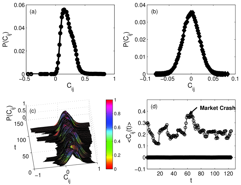
In this section, we analyze the various statistical features of the correlation matrix of 473 daily stock returns listed on the Korean stock markets from 3 January 1993 to 31 May. 2003 using the random matrix theory and Markowitz portfolio theory. We present the results on the statistical properties of the correlation matrix, such as its distribution, eigenvalue spectrum and entropy of portfolio weights calculated by MPT. Fig. 1(a) and (b) show the distribution of the correlation matrices of the original and random data sets. Fig. 1(c) shows the distribution of correlation matrices calculated by shifting 21 days with 250 data points. Fig. 1(d) displays the average value of correlation matrices of Fig. 1(c). In Fig. 1(a), we find that the distribution of the correlation matrix between stocks for a whole period is positively skewed and shows a significant difference from that for the random interaction in Fig. 1(b). In Fig. 1(c), we show that the distribution of the correlation matrix changes considerably over the whole time. Especially, in Fig. 1(d), during the Asian currency crisis, the mean values of the correlation coefficients significantly increased. In other words, the dynamically changes were caused by the complex behavior of the market crash, unlike the case of random interactions. Our findings confirm that all the possible interactions in the Korean stock market deviated from those for the random interaction.

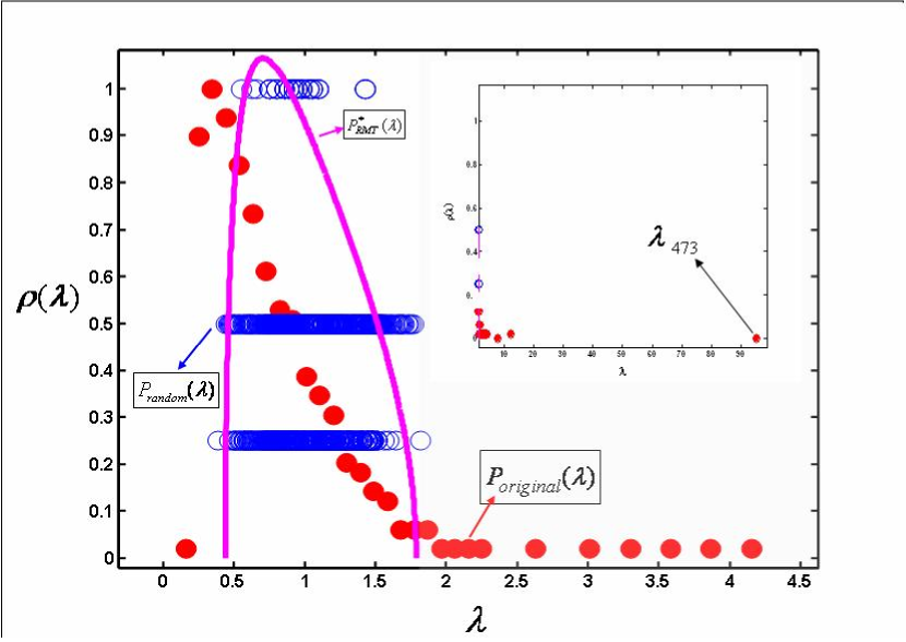
We next decompose the original correlation matrix into the random $C_{random}$ and filter $C_{filter}$ parts using the RMT method to extract the meaningful information from the original correlation matrix. Fig. 2 shows the eigenvalue distribution of the correlation matrix in the Korean stock market. In Fig. 2, the solid-line (orange) is the eigenvalue spectrum predicted by the RMT, and the red circles and blue circles indicate the eigenvalue distributions of the original time series and random data sets, respectively. In Fig. 2, we find that the eigenvalue distribution of the RMT method is very similar to one from the random data, while that for the real time series significantly shows different behavior. Moreover, the largest eigenvalue is 52 times larger than the largest eigenvalue of the RMT. The large values are greater than 25 times those in the United States stock market Plerou2 .

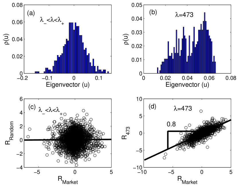
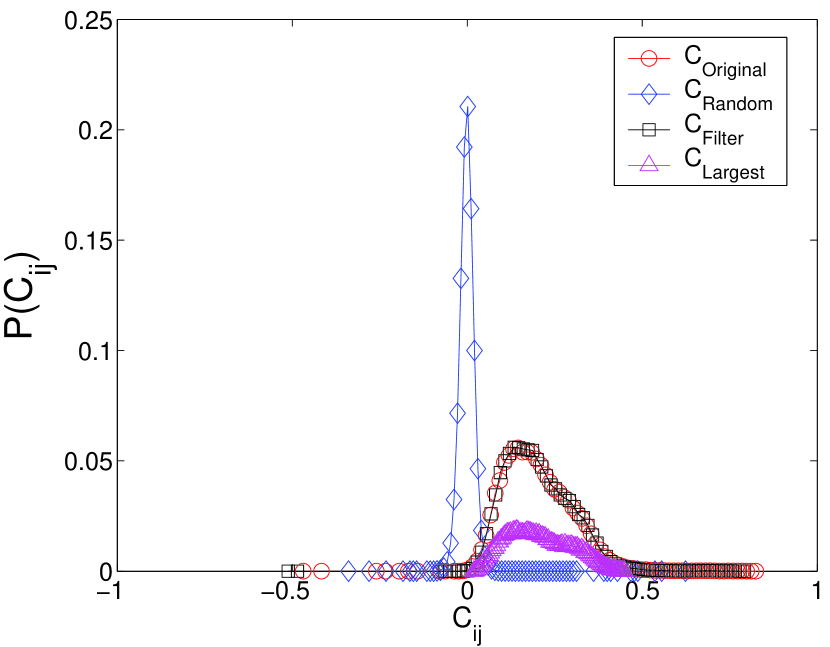
To characterize the statistical properties of each eigenvalues, we created the return time series using equation 8 and calculated the slopes $\beta$ between those and the KOSPI market index using equation 9. Fig. 3(a) and (b) shows the distribution of the eigenvector elements corresponding to both the largest eigenvalue, $\lambda_{473}$ and $\lambda_{100}$, one of eigenvalues of the RMT, respectively. Fig. 3(c) and (d) show the $\beta$ coefficient between the KOSPI market index and the time series created. We find that the $\beta_{473}$ between the market index and time series is 0.8, while one from the time series created using the eigenvector elements predicted by the RMT is approximately zero. We argue that the largest eigenvalue can explain the market properties well, but one from the ranges predicted by the RMT is uncorrelated to the market index. We also decomposed the original correlation matrix according to each eigenvalue divided by the RMT method. Fig. 4 shows the distribution of various correlation matrices. The red circles, blue diamonds, black squares and pink triangles indicate the correlation matrices of the original, random, filter and largest eigenvalues, respectively. Through the above findings, we can expect that the distribution of the random correlation matrix $C_{random}$ follows a Gaussian distribution, while the correlation matrix $C_{filter}$ estimated after removing the random components from the original correlation matrix by the RMT method has a similar distribution as the original time series. We found that the correlation matrix reflecting the largest eigenvalue property has an obvious difference from that of the original time series.

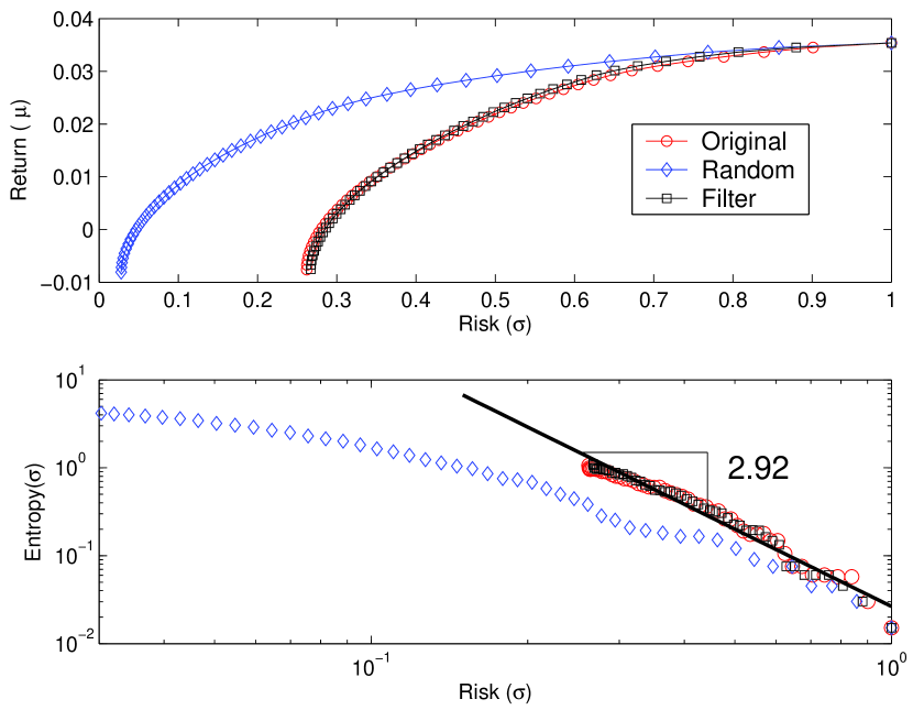
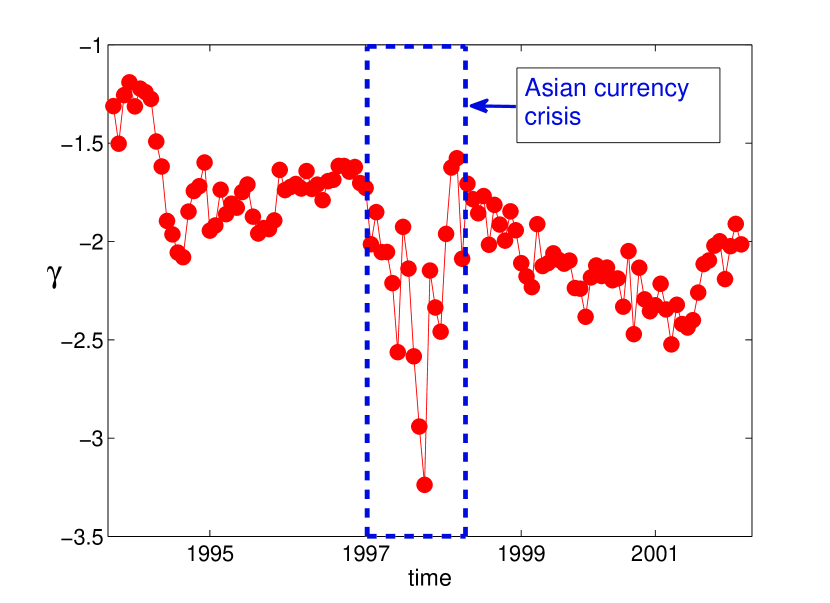
To apply the RMT method to a portfolio optimization problem, we analyzed the portfolio weights estimated by the MPT through various correlation matrices. The important parameters are the return, $\mu_{i}$, standard deviation, $\sigma$ and correlation matrix, $C_{ij}$, of the original stock returns, which are needed to calculate the portfolio weights of each stock. To calculate the effects of the correlation matrix among the input parameters, we apply the correlation matrices, $C_{filter}$, and $C_{random}$ divided by the RMT method. Fig. 5(a) shows the efficient portfolio lines created using the various correlation matrices, such as $C_{original}$, $C_{random}$, and $C_{filter}$. In Fig. 5 (a), we found that the efficient frontier lines calculated with both the original $C_{original}$ and filtered correlation matrices $C_{filter}$ show very similar behavior, while that of the random correlation matrix $C_{random}$ shows significant difference from the original correlation. In addition, the efficient portfolio frontier line of the random correlation matrix $C_{random}$ at a given portfolio risk $\sigma$ overestimates the portfolio return, $\mu$, by a greater amount than one of the original correlation matrix. We next calculated the entropy of the portfolio weights with each correlation matrix, such as $C_{original}$, $C_{filter}$ and $C_{random}$. Fig. 5(b) shows the relationship between the portfolio risk, $\sigma$, and the entropy of the portfolio weights for three types of correlation matrices according to a log-log plot. We found that the entropy($\sigma$) for both the original and filtered correlation matrices was approximately consistent with a power-law function, $E(\sigma)\sim\sigma^{-\gamma}$ with the exponent $\gamma\sim 2.92$, while there is no the power-law function in the relationship between the entropy and the portfolio return, $\mu$ and presented in Fig 5(c). We also calculated the exponents for each sub-periods by shifting 20 days with 500 data points to verify the stability over time the result observed in Fig. 5. We find that while the relationship between entropy of each portfolio weight and portfolio risk follow a power-law function, the exponent values, $\gamma$, calculated from each sub-periods changes over time and lie within $1.19\leq\gamma\leq 3.23$. Especially, the $\gamma$ value calculated during the Asian currency crisis decreases significantly.

IV Conclusions

We investigated the statistical properties of the correlation matrix between the return time series of individual stocks traded in the Korean stock market using the RMT method and observed the effect of the correlation matrix applied to the Markowitz portfolio theory. We found that the distribution of the correlation matrix between stocks showed a positive skew and dynamically changed over time. We found that the eigenvalue distribution of the correlation matrix deviated from those of the RMT, and the largest eigenvalue was 52 times larger than the eigenvalues predicted by the RMT. The slopes $\beta$ between market index and the time series corresponding to the largest eigenvalue were 0.8, while those for the RMT were approximately zero. Notably, we found that the entropy function $E(\sigma)$ of portfolio weights with the portfolio risk $\sigma$ was consistent with a power-law function, $E(\sigma)\sim\sigma^{-\gamma}$, with the exponent $\gamma\sim 2.92$, while the relationship between the entropy and portfolio return $\mu$ is not a power-law function. We find that while for all sub-periods the exponents calculated from the relationship between entropy of each portfolio weight and portfolio risk follow a power-law function, those for sub-periods changed over time and lie within $1.19\leq\gamma\leq 3.23$. Especially, the exponent $\gamma$ decreases significantly during Asian currency crisis. In the next step, we must rigorously study the portfolio weights of other stock markets because these play an important role in terms of the portfolio risk and return.

Figure 1: (a) and (b) show the distribution of the correlation coefficients between stocks of 473 companies of taken from the Korean stock market and random data, respectively. (c) displays the distribution of the correlation matrices of the sub-periods by shifting 21 days with 251 data points and (d) shows the average values of each correlation matrix in (c)

Figure 2: The distribution of the eigenvalues for correlation matrix estimated using the 473 companies listed on the Korean stock market, random data following the iid(0,1) process, and that predicted by the RMT method. The red circles, blue circles, and pink solid-line indicate the original time series, random data, and theoretical lines, respectively.

Figure 3: (a) and (b) show the distribution of both eigenvectors corresponding to $\lambda_{100}$ and $\lambda_{473}$, respectively. (c) and (d) display the $\beta$ coefficients between the normalized market index and the time series created by equation (9) for the eigenvalues $\lambda_{100}$ and $\lambda_{473}$. The value of both $\beta_{100}$ and $\beta_{473}$ are zero and $0.8$, respectively.

Figure 4: The distribution of the original correlation matrix, $C_{original}$, and those created by the random matrix theory, $C_{random}$, $C_{filter}$, and $C_{largest}$, respectively. The red circles, blue diamonds, black squares and pink triangles indicate the correlation matrices corresponding to the original, random, filter and largest eigenvalue, respectively.

Figure 5: (a) shows the efficient portfolio frontier lines for the original, $C_{original}$, random, $C_{random}$, and filter correlation matrix,$C_{filter}$, respectively. (b) displays the relationship between the entropy of the portfolio weights and the portfolio risk. (c) displays the relationship between the entropy and the portfolio return.

Figure 6: The exponent of power-law function, $E(\sigma)\sim\sigma^{\gamma}$ estimated by the relationship between the portfolio risks, $\sigma$, and the entropy of portfolio weights.

References

- (1) T. Lux and M. Marchesi, Nature 397, 498 (1999); T. Lux J. Econ. Behav. Organizat. 33, 143 165 (1998).
- (2) R. N. Mantegna et al., Nature, 376, 46 (1995); R. N. Mantegna et al., Nature, 383, 587 (1996); V. Plerou et al., Nature, 421, 130 (2003); X. Gabaix et al., Nature, 423, 267 (2003);
- (3) G. Oh et al., J. Korean Phys. Soc., 48, 197 (2006); Y. Liu et al., Phys. Rev. E, 60, 1390 (1999); K. Yamasaki et al., Proc. Natl. Acad. Sci., 102, 9424 (2005); W. C. Jun et al., Phys. rev. E, 73 066128 (2006);
- (4) R. N. Mantegna and H. E. Stanley, An Introduction to Econophysics: Correlation and Complexity in Finance (Cambridge University Press, Cambridge, U.K., 1999); J-P. Bouchaud, M. Potters Theory of Financial Risk and Derivative Pricing: From Statistical Physics to Risk Management (Cambridge University Press, Cambridge, USA, 2004).
- (5) E. Elton, M. Gruber, Modern Portfolio Theory and Investment Analysis (Wiley, New York, 1981).
- (6) Y. Okhrin, W. Schmid, J. Econometrics 134. 235 (2006).
- (7) D. Sornette, P. Simonetti and J. V. Andersen, Phys. Rep. 335. 19 (2002)
- (8) J. D. Noh, Phys. Rev. E 61. 5981 (2000).
- (9) J. E. Jackson , A User’s Guide to Principal Components ( Wiley-Interscience; New Ed edition, 2003).
- (10) J. E. Gentle, Singular Value Factorization (Berlin: Springer-Verlag, 1998).
- (11) D. F. Morrison, Multivariate Statistical Methods (New York: McGraw-Hill 1990).
- (12) M. L. Mehta, Random Matrices (Academic Press, Boston, 1991).
- (13) E. P. Wigner, Ann. Math. 53, 36 (1951); E. P. Wigner, Proc. Cambridge Philos. Soc. 47, 790 (1951).
- (14) F. J. Dyson, J. Math. Phys. 3, 140 (1962); F. J. Dyson and M. L. Mehta, J. Math. Phys. 4, 701 (1963).
- (15) M. L. Metha, Nucl. Phys., 18 395 (1960); M. L. Mehta and F. J. Dyson, J. Math. Phys. 4, 713 (1963); M. L. Metha, Commun. Math. Phys., 20 245 (1971);
- (16) T. Guhr, A. Mller-Groeling, and H. A. Weidenmller, Phys. Rep. 299, 190 (1998)
- (17) A. M. Sengupta and P. P. Mitra, Phys. Rev. E 60, 3 (1999).
- (18) P. Sba, Phys. Rev. Lett. 91. 19 (2003).
- (19) A. Utsugi, K. Ino, and M. Oshikawa, Phys. Rev. E 70, 026110 (2004).
- (20) T. Guhr and B. Kälberzk, arXiv:cond-mat/0206577 (2002).
- (21) S. Shari, M. Crane, A. Shamaie, H. Ruskin, Physica A 335, 629 (2004).
- (22) L. Laloux, P. Cizeau, J-P. Bouchaud, and M. Potters, Phys. Rev. Lett. 83, 1467 (1999)
- (23) V. Plerou, P. Gopikrishnan, B. Rosenow, L. A. N. Amaral, and H. E. Stanley, Phys. Rev. Lett. 83 1471 (1999).
- (24) V. Plerou, P. Gopikrishnan, B. Rosennow, L. A. N. Amaral, T. Guhr, and H. E. Stanley, Phys. Rev. E 64, 066126 (2002).
- (25) B. Rosenow, V. Plerou, P. Gopikrishnan, L. A. N. Amaral, and H. E. Stanley, Int. J. of Theoret. Appl. Finance 3, 399 (2000).
- (26) P. Gopikrishnan, B. Rosenow, V. Plerou, and H. E. Stanley, Phys. Rev. E 64, 035106 (2001).
- (27) V. Plerou, P. Gopikrishnan, B. Rosenow, L. A. N. Amaral, and H. E. Stanley, Physica A 287, 374 (2000).
- (28) B. Rosenow, P. Gopikrishnan, V. Plerou, and H. E. Stanley, Physica A 314, 762-767 (2002).
- (29) B. Rosenow, P. Gopikrishnan, V. Plerou, and H. E. Stanley, ”Random Matrix Theory and Cross-Correlations of Stock Prices,” in Empirical Science of Financial Fluctuations: The Advent of Econophysics, edited by H. Takayasu (Springer-Verlag, Tokyo, 2002).
- (30) H. M. Markowitz, J. Finance 7, 77 (1952)