Triangularity and Dipole Asymmetry in Heavy Ion Collisions

Derek Teaney and Li Yan Department of Physics and Astronomy, Stony Brook University, Stony Brook, New York 11794-3800, United States
Abstract

We introduce a cumulant expansion to parameterize possible initial conditions in relativistic heavy ion collisions. We show that the cumulant expansion converges and that it can systematically reproduce the results of Glauber type initial conditions. At third order in the gradient expansion, the cumulants characterize the triangularity r3cos3(ϕψ3,3)delimited-⟨⟩superscript𝑟33italic-ϕsubscript𝜓33\left\langle r^{3}\cos 3(\phi-\psi_{3,3})\right\rangle and the dipole asymmetry r3cos(ϕψ1,3)delimited-⟨⟩superscript𝑟3italic-ϕsubscript𝜓13\left\langle r^{3}\cos(\phi-\psi_{1,3})\right\rangle of the initial entropy distribution. We show that for mid-peripheral collisions the orientation angle of the dipole asymmetry ψ1,3subscript𝜓13\psi_{1,3} has a 20%percent2020\% preference out of plane. This leads to a small net v1subscript𝑣1v_{1} out of plane. In peripheral and mid-central collisions the orientation angles ψ1,3subscript𝜓13\psi_{1,3} and ψ3,3subscript𝜓33\psi_{3,3} are strongly correlated, but this correlation disappears towards central collisions. We study the ideal hydrodynamic response to these cumulants and determine the associated v1/ϵ1subscript𝑣1subscriptitalic-ϵ1v_{1}/\epsilon_{1} and v3/ϵ3subscript𝑣3subscriptitalic-ϵ3v_{3}/\epsilon_{3} for a massless ideal gas equation of state. The space time development of v1subscript𝑣1v_{1} and v3subscript𝑣3v_{3} is clarified with figures. These figures show that v1subscript𝑣1v_{1} and v3subscript𝑣3v_{3} develop towards the edge of the nucleus, and consequently the final spectra are more sensitive to the viscous dynamics of freezeout. The hydrodynamic calculations for v3subscript𝑣3v_{3} are provisionally compared to Alver and Roland fit of STAR inclusive two particle correlation functions. Finally, we propose to measure the v1subscript𝑣1v_{1} associated with the dipole asymmetry and the correlations between ψ1,3subscript𝜓13\psi_{1,3} and ψ3,3subscript𝜓33\psi_{3,3} by measuring a two particle correlation with respect to the participant plane, cos(ϕα3ϕβ+2ΨPP)delimited-⟨⟩subscriptitalic-ϕ𝛼3subscriptitalic-ϕ𝛽2subscriptΨ𝑃𝑃\left\langle\cos(\phi_{\alpha}-3\phi_{\beta}+2\Psi_{PP})\right\rangle. The hydrodynamic prediction for this correlation function is several times larger than a correlation currently measured by the STAR collaboration, cos(ϕα+ϕβ2ΨPP)delimited-⟨⟩subscriptitalic-ϕ𝛼subscriptitalic-ϕ𝛽2subscriptΨ𝑃𝑃\left\langle\cos(\phi_{\alpha}+\phi_{\beta}-2\Psi_{PP})\right\rangle. This experimental measurement would provide convincing evidence for the hydrodynamic and geometric interpretation of two particle correlations at RHIC.

I Introduction

In a recent and significant paper B. Alver and G. Roland (AR) Alver:2010gr provided the most compelling explanation to date for the striking features measured in two particle correlations at the Relativistic Heavy Ion Collider Adams:2005ph ; Adare:2007vu ; Alver:2009id ; Abelev:2009qa ; Adamova:2009ah ; Abelev:2008nda . These features (which are described with picturesque names such as the “ridge” and “shoulder”) are said to arise from the collective response to fluctuating initial conditions. Specifically, if the initial conditions are parameterized with a quadrapole and triangular moment, the two particle correlations reflect the response of the nuclear medium to these anisotropies. The work of AR was motivated in part by event by event simulations of heavy ion collisions with ideal hydrodynamics which showed that the flow from fluctuating initial conditions can describe the general features of the measured two particle correlations Takahashi:2009na . The general idea that the curious correlations are due to a third harmonic in the flow profile was previously suggested by Sorensen Sorensen:2010zq . In addition, many of the features of the observed two particle correlations were found in the AMPT model Lin:2004en ; Ma:2006fm ; Zhang:2007qx , though the geometric nature of these correlations was not understood before the work of Alver and Roland.

The hydrodynamic interpretation of the measured two particle correlations is important for several reasons. First, before this conclusion there was a significant correlation between the measured particles which was not understood. This confusion casted doubt on the hydrodynamic interpretation of RHIC results and clouded the important conclusion that the shear viscosity to entropy ratio of QCD is of order /4πsimilar-toabsentPlanck-constant-over-2-pi4𝜋\sim\hbar/4\pi near the phase transition Teaney:2009qa . However, since the unusual two particle correlations are actually a prediction of hydrodynamics, the observation of these unusual features in the data validates hydrodynamics as an appropriate effective theory for heavy ion events and marginalizes other models. Further, once the hydrodynamic interpretation is adopted the measured correlations can be used to constrain the properties of the medium, e.g. the shear viscosity and the Equation of State (EOS). In particular the effect of viscosity was calculated in Refs. Alver:2010dn ; Schenke:2010rr which will be discussed more completely below.

Motivated by these results, the current work will characterize the fluctuating initial conditions with a cumulant expansion. Instead of running hydrodynamics event to event, the linear response to specified cumulants can be calculated with ideal or viscous hydrodynamics. Subsequently, these response functions can be combined with a Glauber model for the event-by-event cumulants (and their correlations), and the combined result can be fairly compared to data. At third order in the gradient expansion, the initial condition is parameterized by a radial dependence to the dipole moment, r3cosϕdelimited-⟨⟩superscript𝑟3italic-ϕ\left\langle r^{3}\cos\phi\right\rangle, and the triangularity, r3cos3ϕdelimited-⟨⟩superscript𝑟33italic-ϕ\left\langle r^{3}\cos 3\phi\right\rangle . In Section III we will calculate (with ideal hydrodynamics) how the medium responds to these moments and illustrate how this response develops in space and time. Subsequently in Section IV we will compute the corresponding particle spectra v1(pT)subscript𝑣1subscript𝑝𝑇v_{1}(p_{T}) and v3(pT)subscript𝑣3subscript𝑝𝑇v_{3}(p_{T}) and study the sensitivity to certain model parameters related to freezeout. In Section V.1 we will make a comparison to V3Δ/V2Δsubscript𝑉3Δsubscript𝑉2ΔV_{3\Delta}/V_{2\Delta} as extracted by Alver and Roland in their analysis of two particle correlations. We will also make definite predictions for the dipole asymmetry v1(pT)subscript𝑣1subscript𝑝𝑇v_{1}(p_{T}), which, if confirmed, would firmly establish the geometric nature of the two particle correlations. The comparison to data is not final as the effects of resonance decays, viscosity, and higher cumulants have not been included, Nevertheless, the preliminary comparison will firmly tie the formal cumulant expansion outlined in this paper to the measured correlations. Finally, we will compare our calculations to the recent results of Refs. Petersen:2010cw ; Alver:2010dn ; Schenke:2010rr in Section V.2.

II Cumulant expansion and hydrodynamics at RHIC

II.1 The initial conditions for ideal hydrodynamics

In this paper we will use 2+1212+1 dimensional boost invariant ideal hydrodynamics to simulate RHIC events Ollitrault:1992bk ; Kolb:2003dz ; Teaney:2009qa . Briefly, in ideal hydrodynamics the stress tensor satisfies the constituent relation and the conservation laws:

Tμν=(e+𝒫(e))uμuν+𝒫(e)gμν,μTμν=0,formulae-sequencesuperscript𝑇𝜇𝜈𝑒𝒫𝑒superscript𝑢𝜇superscript𝑢𝜈𝒫𝑒superscript𝑔𝜇𝜈subscript𝜇superscript𝑇𝜇𝜈0T^{\mu\nu}=(e+\mathcal{P}(e))u^{\mu}u^{\nu}+\mathcal{P}(e)g^{\mu\nu}\,,\qquad\nabla_{\mu}T^{\mu\nu}=0\,, (1)

where e𝑒e is the energy density, uμsuperscript𝑢𝜇u^{\mu} is the flow velocity, and the pressure 𝒫𝒫\mathcal{P} is specified by the EOS, 𝒫=𝒫(e)𝒫𝒫𝑒\mathcal{P}=\mathcal{P}(e). We will work in flat space but with coordinates

τ=t2z2,ηs=12log(t+ztz).formulae-sequence𝜏superscript𝑡2superscript𝑧2subscript𝜂𝑠12𝑡𝑧𝑡𝑧\tau=\sqrt{t^{2}-z^{2}}\,,\qquad\eta_{s}=\frac{1}{2}\log\left(\frac{t+z}{t-z}\right)\,.

With the assumption of boost invariance, the hydrodynamic fields are independent of ηssubscript𝜂𝑠\eta_{s} and uη=0superscript𝑢𝜂0u^{\eta}=0. Using the constraint uμuμ=1subscript𝑢𝜇superscript𝑢𝜇1u_{\mu}u^{\mu}=-1, the independent fields which must be determined by solving the conservation laws are

e(τ,𝒙),ux(τ,𝒙)uy(τ,𝒙),𝑒𝜏𝒙superscript𝑢𝑥𝜏𝒙superscript𝑢𝑦𝜏𝒙e(\tau,{\bm{x}})\,,\qquad u^{x}(\tau,{\bm{x}})\,\qquad u^{y}(\tau,{\bm{x}})\,, (2)

where 𝒙𝒙{\bm{x}} denotes two dimensional vectors in the transverse plane. We will specify the initial conditions for the subsequent evolution in what follows. At the initial time τosubscript𝜏𝑜\tau_{o} it is reasonable to assume that flow fields are small, uxuy0similar-to-or-equalssuperscript𝑢𝑥superscript𝑢𝑦similar-to-or-equals0u^{x}\simeq u^{y}\simeq 0. This leaves the initial energy density which must be specified e(τo,x,y)𝑒subscript𝜏𝑜𝑥𝑦e(\tau_{o},x,y). We will specify the initial entropy density s(τo,x,y)𝑠subscript𝜏𝑜𝑥𝑦s(\tau_{o},x,y) with a cumulant expansion and infer the initial energy density from the equation of state.

A typical initial condition might be fairly complicated involving several structures. However, the effect of the shear viscosity is to damp the highest Fourier modes. Thus, after damping the shortest wavelengths, the initial entropy distribution is approximately described by a Gaussian with average squared radius r2delimited-⟨⟩superscript𝑟2\left\langle r^{2}\right\rangle and elliptic eccentricity ϵ2subscriptitalic-ϵ2\epsilon_{2} as has traditionally been used to characterize heavy ion events Ollitrault:1992bk . The damping of the highest Fourier modes is nicely seen in Fig. 1 of a recent preprint Schenke:2010rr . The next paragraphs formalize this description and categorize corrections.

II.2 Cumulants

The Fourier transform of the entropy density for a given initial condition is

d2𝒙ei𝒌𝒙ρ(x)=ρ(𝒌),superscriptd2𝒙superscript𝑒𝑖𝒌𝒙𝜌𝑥𝜌𝒌\int{\rm d}^{2}{\bm{x}}\,e^{i{\bm{k}}\cdot{\bm{x}}}\rho(x)=\rho({\bm{k}})\,, (3)

where ρ(𝒙)=τos(τo,𝒙)/Stot𝜌𝒙subscript𝜏𝑜𝑠subscript𝜏𝑜𝒙subscript𝑆tot\rho({\bm{x}})=\tau_{o}s(\tau_{o},{\bm{x}})/S_{\rm tot} and Stot=τod2𝒙s(τo,𝒙)subscript𝑆totsubscript𝜏𝑜superscriptd2𝒙𝑠subscript𝜏𝑜𝒙S_{\rm tot}=\int\tau_{o}{\rm d}^{2}{\bm{x}}\,s(\tau_{o},{\bm{x}}) is the total entropy per space time rapidity. Since the highest Fourier modes are damped, we will expand the initial distribution in 𝒌𝒌{\bm{k}}. Expanding both sides of Eq. (3) with respect to 𝒌𝒌{\bm{k}},

ρ(𝒌)=1+ikaρ1,a+(ika)(ikb)2!ρ2,ab+,𝜌𝒌1𝑖superscript𝑘𝑎subscript𝜌1𝑎𝑖superscript𝑘𝑎𝑖superscript𝑘𝑏2subscript𝜌2𝑎𝑏\rho({\bm{k}})=1+ik^{a}\rho_{1,a}+\frac{(ik^{a})(ik^{b})}{2!}\rho_{2,ab}+\ldots\,, (4)

we see that ρ(𝒌)𝜌𝒌\rho({\bm{k}}) generates moments of the entropy distribution

ρ1,a=xa,ρ2,ab=xaxb,formulae-sequencesubscript𝜌1𝑎delimited-⟨⟩subscript𝑥𝑎subscript𝜌2𝑎𝑏delimited-⟨⟩subscript𝑥𝑎subscript𝑥𝑏\rho_{1,a}=\left\langle x_{a}\right\rangle\,,\qquad\rho_{2,ab}=\left\langle x_{a}x_{b}\right\rangle\,, (5)

where the average is appropriately defined

=d2𝒙ρ(𝒙).delimited-⟨⟩superscriptd2𝒙𝜌𝒙\left\langle\ldots\right\rangle=\int{\rm d}^{2}{\bm{x}}\rho({\bm{x}})\ldots\,. (6)

Although we could classify the initial conditions with these moments, a cumulant expansion seems more natural since the average Glauber distribution is roughly Gaussian and the cumulants are translationally invariant. We therefore define W(𝒌)𝑊𝒌W({\bm{k}})

exp(W(𝒌))d2𝒙ei𝒌𝒙ρ(𝒙),𝑊𝒌superscriptd2𝒙superscript𝑒𝑖𝒌𝒙𝜌𝒙\exp(W({\bm{k}}))\equiv\int{\rm d}^{2}{\bm{x}}\,e^{i{\bm{k}}\cdot{\bm{x}}}\rho({\bm{x}})\,, (7)

and expand both sides in a fourier series

W(𝒌)=1+ikaW1,a+12!(ika)(ika)W2,ab+.𝑊𝒌1𝑖superscript𝑘𝑎subscript𝑊1𝑎12𝑖superscript𝑘𝑎𝑖superscript𝑘𝑎subscript𝑊2𝑎𝑏W({\bm{k}})=1+ik^{a}W_{1,a}+\frac{1}{2!}(ik^{a})(ik^{a})W_{2,ab}+\ldots\,. (8)

From this expansion we see that W(𝒌)𝑊𝒌W({\bm{k}}) is the generating function of cumulants of the underlying distribution ρ(𝒌)𝜌𝒌\rho({\bm{k}})

W1,l=xl,W2,ab=xaxbxaxb.formulae-sequencesubscript𝑊1𝑙delimited-⟨⟩subscript𝑥𝑙subscript𝑊2𝑎𝑏delimited-⟨⟩subscript𝑥𝑎subscript𝑥𝑏delimited-⟨⟩subscript𝑥𝑎delimited-⟨⟩subscript𝑥𝑏W_{1,l}=\left\langle x_{l}\right\rangle\,,\qquad W_{2,ab}=\left\langle x_{a}x_{b}\right\rangle-\left\langle x_{a}\right\rangle\left\langle x_{b}\right\rangle\,. (9)

From now on we will shift the origin so that xa=0delimited-⟨⟩subscript𝑥𝑎0\left\langle x_{a}\right\rangle=0, and the distribution is approximately Gaussian to quadratic order

ρ(𝒌)=exp(12kakbW2,ab).𝜌𝒌12superscript𝑘𝑎superscript𝑘𝑏subscript𝑊2𝑎𝑏\rho({\bm{k}})=\exp\left(-\frac{1}{2}k^{a}k^{b}W_{2,ab}\right)\,. (10)

Higher order corrections in this expansion will correct the distribution away from the Gaussian. The tensor W2,absubscript𝑊2𝑎𝑏W_{2,ab} is a reducible tensor and should be decomposed into irreducible components,

W2,ab=12W2,ccδab+(W2,ab12W2,ccδab).subscript𝑊2𝑎𝑏12subscript𝑊2𝑐𝑐subscript𝛿𝑎𝑏subscript𝑊2𝑎𝑏12subscript𝑊2𝑐𝑐subscript𝛿𝑎𝑏W_{2,ab}=\frac{1}{2}W_{2,cc}\delta_{ab}+\left(W_{2,ab}-\frac{1}{2}W_{2,cc}\delta_{ab}\right)\,. (11)

We orient the x,y𝑥𝑦x,y axes to the participant plane Alver:2006wh where W2,xy=0subscript𝑊2𝑥𝑦0W_{2,xy}=0. Then the irreducible moments are

W2,aa=subscript𝑊2𝑎𝑎absent\displaystyle W_{2,aa}= x2+y2,delimited-⟨⟩superscript𝑥2superscript𝑦2\displaystyle\left\langle x^{2}+y^{2}\right\rangle\,, (12)
W2,xx12Wccδxxsubscript𝑊2𝑥𝑥12subscript𝑊𝑐𝑐subscript𝛿𝑥𝑥\displaystyle W_{2,xx}-\frac{1}{2}W_{cc}\delta_{xx} =12x2y2.absent12delimited-⟨⟩superscript𝑥2superscript𝑦2\displaystyle=\frac{1}{2}\left\langle x^{2}-y^{2}\right\rangle\,. (13)

Clearly the irreducible components of the cumulant expansion are related to the traditional parameters of heavy ion physics:

x2+y2,andϵ2y2x2r2.delimited-⟨⟩superscript𝑥2superscript𝑦2andsubscriptitalic-ϵ2delimited-⟨⟩superscript𝑦2superscript𝑥2superscript𝑟2\displaystyle\left\langle x^{2}+y^{2}\right\rangle\,,\qquad\mbox{and}\qquad\epsilon_{2}\equiv\frac{\left\langle y^{2}-x^{2}\right\rangle}{r^{2}}\,. (14)

To write down corrections to these results it is more convenient and illustrative to use cylindrical tensors rather than Cartesian tensors. Appendix A develops this expansion in detail and only certain features will be summarized here. Appendix A.1 expands W(𝒌)𝑊𝒌W({\bm{k}}) in a Fourier series:

W(𝒌)=W0(k)+2n=1Wnc(k)cos(ϕk)+2n=1Wns(k)sin(nϕk),𝑊𝒌subscript𝑊0𝑘2superscriptsubscript𝑛1superscriptsubscript𝑊𝑛𝑐𝑘subscriptitalic-ϕ𝑘2superscriptsubscript𝑛1superscriptsubscript𝑊𝑛𝑠𝑘𝑛subscriptitalic-ϕ𝑘W({\bm{k}})=W_{0}(k)+2\sum_{n=1}^{\infty}W_{n}^{c}(k)\cos(\phi_{k})+2\sum_{n=1}^{\infty}W_{n}^{s}(k)\sin(n\phi_{k})\,, (15)

where k𝑘k and ϕ𝒌subscriptitalic-ϕ𝒌\phi_{\bm{k}} are the norm and azimuthal angle of the momentum vector. The Wnc,s(k)superscriptsubscript𝑊𝑛𝑐𝑠𝑘W_{n}^{c,s}(k) are also expanded in k𝑘k to characterize the distribution at largest wavelength:

W0(k)=subscript𝑊0𝑘absent\displaystyle W_{0}(k)= 12!W0,2(ik)2+O(k4),12subscript𝑊02superscript𝑖𝑘2𝑂superscript𝑘4\displaystyle\frac{1}{2!}W_{0,2}(ik)^{2}+O(k^{4})\,, (16a)
W1c(k)=superscriptsubscript𝑊1𝑐𝑘absent\displaystyle W_{1}^{c}(k)= W1,1c+O(k3),superscriptsubscript𝑊11𝑐𝑂superscript𝑘3\displaystyle W_{1,1}^{c}+O(k^{3})\,, (16b)
W1s(k)=superscriptsubscript𝑊1𝑠𝑘absent\displaystyle W_{1}^{s}(k)= W1,1s+O(k3),superscriptsubscript𝑊11𝑠𝑂superscript𝑘3\displaystyle W_{1,1}^{s}+O(k^{3})\,, (16c)
W2c(k)=superscriptsubscript𝑊2𝑐𝑘absent\displaystyle W_{2}^{c}(k)= 12!W2,2c(ik)2+O(k4),12superscriptsubscript𝑊22𝑐superscript𝑖𝑘2𝑂superscript𝑘4\displaystyle\frac{1}{2!}W_{2,2}^{c}(ik)^{2}+O(k^{4})\,, (16d)
W2s(k)=superscriptsubscript𝑊2𝑠𝑘absent\displaystyle W_{2}^{s}(k)= W2,2s+O(k4).superscriptsubscript𝑊22𝑠𝑂superscript𝑘4\displaystyle W_{2,2}^{s}+O(k^{4})\,. (16e)

After Appendix A we find that to order k2superscript𝑘2k^{2}

W0,2=subscript𝑊02absent\displaystyle W_{0,2}= 12r2,12delimited-⟨⟩superscript𝑟2\displaystyle\frac{1}{2}\left\langle r^{2}\right\rangle\,, (17)
W1,1c=superscriptsubscript𝑊11𝑐absent\displaystyle W_{1,1}^{c}= 0,0\displaystyle 0\,, (18)
W1,1s=superscriptsubscript𝑊11𝑠absent\displaystyle W_{1,1}^{s}= 0,0\displaystyle 0\,, (19)
W2,2c=superscriptsubscript𝑊22𝑐absent\displaystyle W_{2,2}^{c}= 14r2cos(2ϕ),14delimited-⟨⟩superscript𝑟22italic-ϕ\displaystyle\frac{1}{4}\left\langle r^{2}\cos(2\phi)\right\rangle\,, (20)
W2,2s=superscriptsubscript𝑊22𝑠absent\displaystyle W_{2,2}^{s}= 0.0\displaystyle 0\,. (21)

Here we have used translational invariance and rotational invariance (as in the Cartesian case) to eliminate W1,1csuperscriptsubscript𝑊11𝑐W_{1,1}^{c}, W1,1ssuperscriptsubscript𝑊11𝑠W_{1,1}^{s}, and W2,2ssuperscriptsubscript𝑊22𝑠W_{2,2}^{s}. To third order in the gradient expansion the dipole terms W1c(k)superscriptsubscript𝑊1𝑐𝑘W_{1}^{c}(k) and W1s(k)superscriptsubscript𝑊1𝑠𝑘W_{1}^{s}(k) are non-zero

W1c(k)=superscriptsubscript𝑊1𝑐𝑘absent\displaystyle W_{1}^{c}(k)= 13!W1,3(ik)3+O(k5),13subscript𝑊13superscript𝑖𝑘3𝑂superscript𝑘5\displaystyle\frac{1}{3!}W_{1,3}(ik)^{3}+O(k^{5})\,, W1,3=subscript𝑊13absent\displaystyle W_{1,3}= 38r3cosϕ,38delimited-⟨⟩superscript𝑟3italic-ϕ\displaystyle\frac{3}{8}\left\langle r^{3}\cos\phi\right\rangle\,, (22a)
W1s(k)=superscriptsubscript𝑊1𝑠𝑘absent\displaystyle W_{1}^{s}(k)= 13!W1,3(ik)3+O(k5),13subscript𝑊13superscript𝑖𝑘3𝑂superscript𝑘5\displaystyle\frac{1}{3!}W_{1,3}(ik)^{3}+O(k^{5})\,, W1,3=subscript𝑊13absent\displaystyle W_{1,3}= 38r3sinϕ.38delimited-⟨⟩superscript𝑟3italic-ϕ\displaystyle\frac{3}{8}\left\langle r^{3}\sin\phi\right\rangle\,. (22b)
Similarly, at third order in the gradient expansion there are terms proportional to cos(3ϕ)3italic-ϕ\cos(3\phi)
W3c(k)=superscriptsubscript𝑊3𝑐𝑘absent\displaystyle W_{3}^{c}(k)= 13!W3,3(ik)3+O(k5),13subscript𝑊33superscript𝑖𝑘3𝑂superscript𝑘5\displaystyle\frac{1}{3!}W_{3,3}(ik)^{3}+O(k^{5})\,, W3,3c=superscriptsubscript𝑊33𝑐absent\displaystyle W_{3,3}^{c}= 18r3cos(3ϕ),18delimited-⟨⟩superscript𝑟33italic-ϕ\displaystyle\frac{1}{8}\left\langle r^{3}\cos(3\phi)\right\rangle\,, (22c)
W3s(k)=superscriptsubscript𝑊3𝑠𝑘absent\displaystyle W_{3}^{s}(k)= 13!W3,3(ik)3+O(k5)13subscript𝑊33superscript𝑖𝑘3𝑂superscript𝑘5\displaystyle\frac{1}{3!}W_{3,3}(ik)^{3}+O(k^{5}) W3,3s=superscriptsubscript𝑊33𝑠absent\displaystyle W_{3,3}^{s}= 18r3sin(3ϕ).18delimited-⟨⟩superscript𝑟33italic-ϕ\displaystyle\frac{1}{8}\left\langle r^{3}\sin(3\phi)\right\rangle\,. (22d)

Once the fourier coefficients Wn,msubscript𝑊𝑛𝑚W_{n,m} are specified, the entropy distribution in space can be found with a fourier transform; see Eqs. 34 and 35 and the surrounding text for further discussion.

II.3 A strategy for event by event hydrodynamics

If the cumulants beyond second order are in some sense small, then the change in the hydrodynamic spectra due to a specified set of higher cumulants is linearly proportional to the deformation

dδNdϕp=n,m,{s,c}[1Wn,mc,sdδNdϕp]n,m,{s,c}Wn,mc,s,d𝛿𝑁dsubscriptitalic-ϕ𝑝subscript𝑛𝑚𝑠𝑐subscriptdelimited-[]1superscriptsubscript𝑊𝑛𝑚𝑐𝑠d𝛿𝑁dsubscriptitalic-ϕ𝑝𝑛𝑚𝑠𝑐superscriptsubscript𝑊𝑛𝑚𝑐𝑠\frac{{\rm d}\delta N}{{\rm d}\phi_{p}}=\sum_{n,m,\left\{s,c\right\}}\left[\frac{1}{W_{n,m}^{c,s}}\frac{{\rm d}\delta N}{{\rm d}\phi_{p}}\right]_{n,m,\left\{s,c\right\}}W_{n,m}^{c,s}\;, (23)

where

[1Wn,mc,sdδNdϕp]n,m,{c,s},subscriptdelimited-[]1superscriptsubscript𝑊𝑛𝑚𝑐𝑠d𝛿𝑁dsubscriptitalic-ϕ𝑝𝑛𝑚𝑐𝑠\left[\frac{1}{W_{n,m}^{c,s}}\frac{{\rm d}\delta N}{{\rm d}\phi_{p}}\right]_{n,m,\left\{c,s\right\}}\,, (24)

is the normalized response to a given cumulant. If the non-linear interactions between the elliptic flow and the higher cumulants can be ignored (i.e. the elliptic flow is sufficiently small), then the background Gaussian is approximately radially symmetric and the response of the sin\sin terms are related to the response of the cosine terms through a rotation. In this case, we are free to rotate our coordinate system by an angle ψn,msubscript𝜓𝑛𝑚\psi_{n,m}

ψn,m=1natan2(Wn,ms,Wn,mc)+πn,subscript𝜓𝑛𝑚1𝑛atan2superscriptsubscript𝑊𝑛𝑚𝑠superscriptsubscript𝑊𝑛𝑚𝑐𝜋𝑛\psi_{n,m}=\frac{1}{n}{\rm atan2}(W_{n,m}^{s},W_{n,m}^{c})+\frac{\pi}{n}\,, (25)

so that the sin\sin terms vanish. In this rotated frame (which we will notate as W^^𝑊\hat{W}) the cumulants are

W^n,ms=0,W^n,mc=(Wn,mc)2+(Wn,ms)2,formulae-sequencesuperscriptsubscript^𝑊𝑛𝑚𝑠0superscriptsubscript^𝑊𝑛𝑚𝑐superscriptsuperscriptsubscript𝑊𝑛𝑚𝑐2superscriptsuperscriptsubscript𝑊𝑛𝑚𝑠2\hat{W}_{n,m}^{s}=0\,,\qquad\hat{W}_{n,m}^{c}=-\sqrt{(W_{n,m}^{c})^{2}+(W_{n,m}^{s})^{2}}\,, (26)

and the spectrum can be written

dδNdϕp=n,m,c[1W^n,mcdδNd(ϕpψn,m)]n,m,{c}W^n,mc.d𝛿𝑁dsubscriptitalic-ϕ𝑝subscript𝑛𝑚𝑐subscriptdelimited-[]1superscriptsubscript^𝑊𝑛𝑚𝑐d𝛿𝑁dsubscriptitalic-ϕ𝑝subscript𝜓𝑛𝑚𝑛𝑚𝑐superscriptsubscript^𝑊𝑛𝑚𝑐\frac{{\rm d}\delta N}{{\rm d}\phi_{p}}=\sum_{n,m,c}\left[\frac{1}{\hat{W}_{n,m}^{c}}\frac{{\rm d}\delta N}{{\rm d}(\phi_{p}-\psi_{n,m})}\right]_{n,m,\left\{c\right\}}\hat{W}_{n,m}^{c}\,. (27)

Thus, the assumption of a rotationally invariant background reduces the number of coefficients by a factor of two.

In this paper we will assume that all deformations from spherical are small including the elliptic flow. Thus, we will neglect the non-linear couplings between the elliptic flow and the triangular flow and the elliptic flow and the dipolar flow. We have investigated the influence of the ellipticity on the triangular and dipolar flow and our preliminary findings show that the effect of the elliptic flow on the triangular flow is small. A similar finding was reported in the very recent preprint by the Duke group Qin:2010pf . However, the effect of the elliptic flow on the dipolar flow is non-negligible when the dipole angle is oriented in plane. This complication will be reported on in future work YanWork .

The angle ψ2,2subscript𝜓22\psi_{2,2} specifies the orientation of the participant plane ΨPPsubscriptΨ𝑃𝑃\Psi_{PP}, and the second order cumulant W^2,2subscript^𝑊22\hat{W}_{2,2} determines the ellipticity

ϵ2r2cos2(ϕΨPP)r2=4W^2,2cr2,ΨPPψ2,2.formulae-sequencesubscriptitalic-ϵ2delimited-⟨⟩superscript𝑟22italic-ϕsubscriptΨ𝑃𝑃delimited-⟨⟩superscript𝑟24superscriptsubscript^𝑊22𝑐delimited-⟨⟩superscript𝑟2subscriptΨ𝑃𝑃subscript𝜓22\displaystyle\epsilon_{2}\equiv-\frac{\left\langle r^{2}\cos 2(\phi-\Psi_{PP})\right\rangle}{\left\langle r^{2}\right\rangle}=-\frac{4\hat{W}_{2,2}^{c}}{\left\langle r^{2}\right\rangle}\,,\qquad\Psi_{PP}\equiv\psi_{2,2}\,. (28)

The participant plane angle ΨPPsubscriptΨ𝑃𝑃\Psi_{PP} is distinct from the reaction plane angle which we denote with ΨRsubscriptΨ𝑅\Psi_{R}.

The third order cumulant W^3,3csuperscriptsubscript^𝑊33𝑐\hat{W}_{3,3}^{c} describes the triangularity as introduced by Alver and Roland. These authors suggested a definition of the triangularity and orientation angle ϵ3ARsuperscriptsubscriptitalic-ϵ3𝐴𝑅\epsilon_{3}^{AR} and ψ3ARsuperscriptsubscript𝜓3𝐴𝑅\psi_{3}^{AR} with a quadratic radial weight

ϵ3AR=r2cos(3(ϕΨ3AR))r2,Ψ3AR=13atan2(r2sin(3ϕ),r2cos(3ϕ))+π3.formulae-sequencesuperscriptsubscriptitalic-ϵ3𝐴𝑅delimited-⟨⟩superscript𝑟23italic-ϕsuperscriptsubscriptΨ3𝐴𝑅delimited-⟨⟩superscript𝑟2superscriptsubscriptΨ3𝐴𝑅13atan2delimited-⟨⟩superscript𝑟23italic-ϕdelimited-⟨⟩superscript𝑟23italic-ϕ𝜋3\epsilon_{3}^{AR}=-\frac{\left\langle r^{2}\cos(3(\phi-\Psi_{3}^{AR}))\right\rangle}{\left\langle r^{2}\right\rangle}\,,\qquad\Psi_{3}^{AR}=\frac{1}{3}{\rm atan}2(\left\langle r^{2}\sin(3\phi)\right\rangle,\left\langle r^{2}\cos(3\phi)\right\rangle)+\frac{\pi}{3}\,. (29)

We will abandon this analytically frustrated definition, and define the triangularity ϵ3subscriptitalic-ϵ3\epsilon_{3} and the associated angle with an r3superscript𝑟3r^{3} weight

ϵ3subscriptitalic-ϵ3absent\displaystyle\epsilon_{3}\equiv r3cos3(ϕψ3,3)r3=8W^3,3cr3,delimited-⟨⟩superscript𝑟33italic-ϕsubscript𝜓33delimited-⟨⟩superscript𝑟38superscriptsubscript^𝑊33𝑐delimited-⟨⟩superscript𝑟3\displaystyle-\frac{\left\langle r^{3}\cos 3(\phi-\psi_{3,3})\right\rangle}{\left\langle r^{3}\right\rangle}=-\frac{8\hat{W}_{3,3}^{c}}{\left\langle r^{3}\right\rangle}\,, (30)
ψ3,3subscript𝜓33absent\displaystyle\psi_{3,3}\equiv 13atan2(r3sin3ϕ,r3cos3ϕ)+π3.13atan2delimited-⟨⟩superscript𝑟33italic-ϕdelimited-⟨⟩superscript𝑟33italic-ϕ𝜋3\displaystyle\frac{1}{3}{\rm atan}2(\left\langle r^{3}\sin 3\phi\right\rangle,\left\langle r^{3}\cos 3\phi\right\rangle)+\frac{\pi}{3}\,. (31)

The difference between the r2superscript𝑟2r^{2} and r3superscript𝑟3r^{3} weight is captured by the response of the system to the fifth order cumulants, W3,5c[r5cos3ϕ4r2r3cos3ϕ]proportional-tosuperscriptsubscript𝑊35𝑐delimited-[]delimited-⟨⟩superscript𝑟53italic-ϕ4delimited-⟨⟩superscript𝑟2delimited-⟨⟩superscript𝑟33italic-ϕW_{3,5}^{c}\propto\left[\left\langle r^{5}\cos 3\phi\right\rangle-4\left\langle r^{2}\right\rangle\left\langle r^{3}\cos 3\phi\right\rangle\right] . Recent studies of the response of the system to ϵ5subscriptitalic-ϵ5\epsilon_{5} (or W5,5subscript𝑊55W_{5,5} in the current context) suggests that the response to these fifth order cumulants will be small Alver:2010dn .

The third order cumulant W^1,3csuperscriptsubscript^𝑊13𝑐\hat{W}_{1,3}^{c} describes a dipole asymmetry and also appears to the same order in the gradient expansion. By analogy we define ϵ1subscriptitalic-ϵ1\epsilon_{1} and ψ1,3subscript𝜓13\psi_{1,3}

ϵ1subscriptitalic-ϵ1absent\displaystyle\epsilon_{1}\equiv r3cos(ϕψ1,3)r3=83W^1,3cr3,delimited-⟨⟩superscript𝑟3italic-ϕsubscript𝜓13delimited-⟨⟩superscript𝑟383superscriptsubscript^𝑊13𝑐delimited-⟨⟩superscript𝑟3\displaystyle-\frac{\left\langle r^{3}\cos(\phi-\psi_{1,3})\right\rangle}{\left\langle r^{3}\right\rangle}=-\frac{8}{3}\frac{\hat{W}_{1,3}^{c}}{\left\langle r^{3}\right\rangle}\,, (32)
ψ1,3subscript𝜓13absent\displaystyle\psi_{1,3}\equiv atan2(r3sinϕ,r3cosϕ)+π.atan2delimited-⟨⟩superscript𝑟3italic-ϕdelimited-⟨⟩superscript𝑟3italic-ϕ𝜋\displaystyle{\rm atan}2(\left\langle r^{3}\sin\phi\right\rangle,\left\langle r^{3}\cos\phi\right\rangle)+\pi\,. (33)

Estimates for these parameters and their correlations will be given in the next section.

II.4 The dipole asymmetry and triangularity

To get a feeling for the dipole asymmetry and triangularity we first record the explicit coordinate space expressions for a distribution with only triangularity

s(𝒙,τ)[1+r3ϵ324((x)33(y)2x)]er2r2,proportional-to𝑠𝒙𝜏delimited-[]1delimited-⟨⟩superscript𝑟3subscriptitalic-ϵ324superscript𝑥33superscript𝑦2𝑥superscript𝑒superscript𝑟2delimited-⟨⟩superscript𝑟2s({\bm{x}},\tau)\propto\left[1+\frac{\left\langle r^{3}\right\rangle\epsilon_{3}}{24}\left(\left(\frac{\partial}{\partial x}\right)^{3}-3\left(\frac{\partial}{\partial y}\right)^{2}\frac{\partial}{\partial x}\right)\right]e^{-\frac{r^{2}}{\left\langle r^{2}\right\rangle}}\,, (34)

and a distribution with only a dipole asymmetry

s(𝒙,τ)[1+r3ϵ18((x)3+(y)2x)]er2r2.proportional-to𝑠𝒙𝜏delimited-[]1delimited-⟨⟩superscript𝑟3subscriptitalic-ϵ18superscript𝑥3superscript𝑦2𝑥superscript𝑒superscript𝑟2delimited-⟨⟩superscript𝑟2s({\bm{x}},\tau)\propto\left[1+\frac{\left\langle r^{3}\right\rangle\epsilon_{1}}{8}\left(\left(\frac{\partial}{\partial x}\right)^{3}+\left(\frac{\partial}{\partial y}\right)^{2}\frac{\partial}{\partial x}\right)\right]e^{-\frac{r^{2}}{\left\langle r^{2}\right\rangle}}\,. (35)

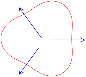
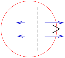
Here the orientation angles ψ3,3subscript𝜓33\psi_{3,3} and ψ1,3subscript𝜓13\psi_{1,3} are set to zero. At large enough radius the derivative terms become large and overwhelm the leading term making the distribution negative. This is an unavoidable consequence of truncating a cumulant expansion at any finite order. As explained in Appendix A we regulate these terms and adjust the overall constant to reproduce the total entropy in a central RHIC collision. Fig. 1a and Fig. 1b illustrate initial conditions with net triangularity and net dipole asymmetry respectively. The distribution with net triangularity leads to a v3(pT)subscript𝑣3subscript𝑝𝑇v_{3}(p_{T}) while the dipole asymmetry leads to a v1(pT)subscript𝑣1subscript𝑝𝑇v_{1}(p_{T}).

Refer to caption
Refer to caption
Figure 1: A schematic of an event with (a) net triangularity and (b) net dipole asymmetry. The triangularity produces a net v3(pT)subscript𝑣3subscript𝑝𝑇v_{3}(p_{T}) and the dipole asymmetry produces a net v1(pT)subscript𝑣1subscript𝑝𝑇v_{1}(p_{T}). The cross in (b) indicates the center of entropy (analogous to the center of mass) and the large arrow indicates the orientation of the dipole.

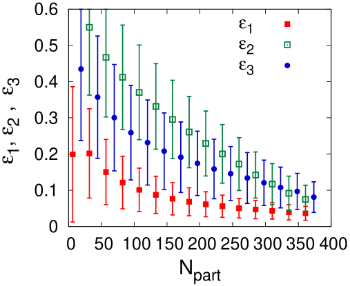
To estimate these parameters and their correlations we have used the PHOBOS monte carlo Glauber code Alver:2008aq . Fig. 2 shows the distribution of ϵ1subscriptitalic-ϵ1\epsilon_{1}, ϵ2subscriptitalic-ϵ2\epsilon_{2} and ϵ3subscriptitalic-ϵ3\epsilon_{3} as a function of the number of participants. We see that the dipole asymmetry is about a factor of two smaller than the triangularity but is not negligibly small.
Refer to caption
Figure 2: Size of the moments ϵ1subscriptitalic-ϵ1\epsilon_{1}, ϵ2subscriptitalic-ϵ2\epsilon_{2} and ϵ3subscriptitalic-ϵ3\epsilon_{3} as a function of the number of participants. The points indicate the average value of ϵndelimited-⟨⟩delimited-⟨⟩subscriptitalic-ϵ𝑛\langle\!\langle\epsilon_{n}\rangle\!\rangle and the errorbars indicate the variance of ϵnsubscriptitalic-ϵ𝑛\epsilon_{n} at fixed Npartsubscript𝑁partN_{\rm part}.

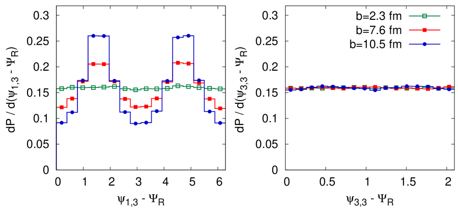
Fig. 3 shows the distribution of ψ1,3subscript𝜓13\psi_{1,3} and ψ3,3subscript𝜓33\psi_{3,3} with respect to reaction plane at various impact parameters. We see that although ψ3,3subscript𝜓33\psi_{3,3} is uncorrelated with respect to the reaction plane, ψ1,3subscript𝜓13\psi_{1,3} shows an anti-correlation with respect to the reaction plane, which eventually disappears toward central collisions.
Refer to caption
Figure 3: Distribution of the angles ψ1,3subscript𝜓13\psi_{1,3} and ψ3,3subscript𝜓33\psi_{3,3} with respect to the reaction plane for three different impact parameters.

More importantly, the angles ψ1,3subscript𝜓13\psi_{1,3} and ψ3,3subscript𝜓33\psi_{3,3} are strongly correlated in mid central collisions (a similar observation was made recently by Staig and Shuryak Staig:2010pn ). Fig. 4 shows the conditional probability distribution, i.e.
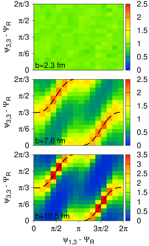
P(ψ3,3|ψ1,3,ΨR)The probability of ψ3,3 given ψ1,3 and ΨR.𝑃conditionalsubscript𝜓33subscript𝜓13subscriptΨ𝑅The probability of ψ3,3 given ψ1,3 and ΨRP(\psi_{3,3}|\psi_{1,3},\Psi_{R})\equiv\mbox{The probability of $\psi_{3,3}$ given $\psi_{1,3}$ and $\Psi_{R}$}.
Refer to caption
Figure 4: The conditional probability distribution P(ψ3,3|ψ1,3ΨR)𝑃conditionalsubscript𝜓33subscript𝜓13subscriptΨ𝑅P(\psi_{3,3}|\psi_{1,3}\Psi_{R}) for three different impact parameters b=0,7.6,10.5𝑏07.610.5b=0,7.6,10.5 fm. The functional form of the dashed curve is given by Eq. (40) with fit parameter C=0.53𝐶0.53C=0.53 for b=7.6fm𝑏7.6fmb=7.6\,{\rm fm} and C=0.56𝐶0.56C=0.56 for b=10.5fm𝑏10.5fmb=10.5\,{\rm fm}.

The strong correlation may be explained physically as follows. When the dipole asymmetry is in plane then the triangular axis is at π/3𝜋3\pi/3, i.e. the point of the triangle is aligned with the dipole axis as exhibited in Fig. 5(a). However, when the dipole axis is out of plane then the triangular axis is also out of plane as exhibited in Fig. 5(b).

Refer to caption
Figure 5: The figure qualitatively describes the fluctuations associated with the Glauber model as illustrated in Fig. 4. When the dipole asymmetry is in plane (Position A), then the tip of triangularity is aligned with dipole asymmetry. When the dipole asymmetry is out of plane (Position B), the tip of the triangle is anti-aligned with the dipole asymmetry.

These correlations are a reflection of the almond shape geometry and their general form can be established by symmetry arguments. First, since the probability of finding a dipole asymmetry in a given quadrant of the ellipse is the same for every quadrant, the probability distributions dP/d(ψ1,3ΨR)d𝑃dsubscript𝜓13subscriptΨ𝑅{\rm d}P/{\rm d}(\psi_{1,3}-\Psi_{R}) must only involve even cosine terms

dPdψ1,3=12π(12Acos2(ψ1,3ΨR))+).\frac{{\rm d}P}{{\rm d}\psi_{1,3}}=\frac{1}{2\pi}\left(1-2A\cos 2(\psi_{1,3}-\Psi_{R}))+\ldots\right)\,. (36)

The sign has been chosen so that a positive A𝐴A coefficient describes the out-of plane preference seen in Fig. 3. The coefficient A𝐴A must vanish in a cylindrically symmetric collision, and for small anisotropy we have

Aϵ2,proportional-to𝐴delimited-⟨⟩delimited-⟨⟩subscriptitalic-ϵ2A\propto\langle\!\langle\epsilon_{2}\rangle\!\rangle\,, (37)

where the double brackets denotes an event averaged ϵ2subscriptitalic-ϵ2\epsilon_{2} Similarly dP/d(ψ3,3ΨR)d𝑃dsubscript𝜓33subscriptΨ𝑅{\rm d}P/{\rm d}(\psi_{3,3}-\Psi_{R}) must involve even cosine terms and must be 2π/32𝜋32\pi/3 periodic

dPd(ψ3,3ΨR)=12π(1+2A6cos(6(ψ3,3ΨR))+).d𝑃dsubscript𝜓33subscriptΨ𝑅12𝜋12subscript𝐴66subscript𝜓33subscriptΨ𝑅\frac{{\rm d}P}{{\rm d}(\psi_{3,3}-\Psi_{R})}=\frac{1}{2\pi}\left(1+2A_{6}\cos(6(\psi_{3,3}-\Psi_{R}))+\ldots\right)\,. (38)

The relatively high fourier number n=6𝑛6n=6 explains the smallness of the observed asymmetry, and A6subscript𝐴6A_{6} will be ignored from now on. The form of the conditional probability distribution can also be established based on general considerations. Appendix B uses symmetry arguments, a fourier expansion, and the statement that the correlation is strongest when the triangle and dipole angles are aligned at π/2𝜋2\pi/2 out of plane, to establish a three parameter functional form which describes the correlations fairly well

P(ψ3,3|ψ1,3,ΨR)=12π[12(B02B2cos(2ψ1,32ΨR))cos(3ψ3,3ϕ2ΨR)],𝑃conditionalsubscript𝜓33subscript𝜓13subscriptΨ𝑅12𝜋delimited-[]12subscript𝐵02subscript𝐵22subscript𝜓132subscriptΨ𝑅3subscript𝜓33superscriptitalic-ϕ2subscriptΨ𝑅P(\psi_{3,3}|\psi_{1,3},\Psi_{R})=\frac{1}{2\pi}\Big{[}1-2\left(B_{0}-2B_{2}\cos(2\psi_{1,3}-2\Psi_{R})\,\right)\cos(3\psi_{3,3}-\phi^{*}-2\Psi_{R})\Big{]}\,, (39)

where

ϕ=ψ1,3Csin(2ψ1,32ΨR).superscriptitalic-ϕsubscript𝜓13𝐶2subscript𝜓132subscriptΨ𝑅\phi^{*}=\psi_{1,3}-C\sin(2\psi_{1,3}-2\Psi_{R})\,. (40)

The signs are chosen so that B0subscript𝐵0B_{0}, B2subscript𝐵2B_{2}, and C𝐶C are positive constants in the final fits. A sample fit with this functional form is given in Fig. 16 of Appendix B. The phase angle ϕsuperscriptitalic-ϕ\phi^{*} is illustrated by the dashed black line in Fig. 4, which is found by solving 3ψ3,3ϕ+2ΨR=π3subscript𝜓33superscriptitalic-ϕ2subscriptΨ𝑅𝜋3\psi_{3,3}-\phi^{*}+2\Psi_{R}=\pi for ψ3,3subscript𝜓33\psi_{3,3}. Although we have written the conditional probability when the reaction plane angle is fixed, the same arguments could have been used to determine the functional form of the conditional probability when the participant plane angle is fixed, i.e.

P(ψ3,3|ψ1,3ΨPP)=Eq. (39) with ΨRΨPP and sightly different numerical coefficients.𝑃conditionalsubscript𝜓33subscript𝜓13subscriptΨ𝑃𝑃Eq. (39) with ΨRΨPP and sightly different numerical coefficientsP(\psi_{3,3}|\psi_{1,3}\Psi_{PP})=\mbox{Eq.~{}(\ref{p1p3pr}) with $\Psi_{R}\rightarrow\Psi_{PP}$ and sightly different numerical coefficients}. (41)

In the limit of small elliptic eccentricity the coefficients scale as

B0ϵ2,B2ϵ22,Cϵ2,formulae-sequenceproportional-tosubscript𝐵0delimited-⟨⟩delimited-⟨⟩subscriptitalic-ϵ2formulae-sequenceproportional-tosubscript𝐵2superscriptdelimited-⟨⟩delimited-⟨⟩subscriptitalic-ϵ22proportional-to𝐶delimited-⟨⟩delimited-⟨⟩subscriptitalic-ϵ2B_{0}\propto\langle\!\langle\epsilon_{2}\rangle\!\rangle\,,\qquad B_{2}\propto\langle\!\langle\epsilon_{2}\rangle\!\rangle^{2}\,,\qquad C\propto\langle\!\langle\epsilon_{2}\rangle\!\rangle\,, (42)

as is shown in Appendix B. Thus the conditional probability distribution simplifies in this limit to

P(ψ3,3|ψ1,3ΨR)=12π[12B0cos(3ψ3,3ψ1,32ΨR)],𝑃conditionalsubscript𝜓33subscript𝜓13subscriptΨ𝑅12𝜋delimited-[]12subscript𝐵03subscript𝜓33subscript𝜓132subscriptΨ𝑅P(\psi_{3,3}|\psi_{1,3}\Psi_{R})=\frac{1}{2\pi}\left[1-2B_{0}\cos(3\psi_{3,3}-\psi_{1,3}-2\Psi_{R})\right], (43)

which describes almost all of the essential physical features.

The strong correlation means that if the triangular and the participant planes are known, then the dipole plane can be determined statistically. The probability distribution of ψ1,3subscript𝜓13\psi_{1,3} for fixed ψ3,3subscript𝜓33\psi_{3,3} and ΨPPsubscriptΨ𝑃𝑃\Psi_{PP} is approximately

P(ψ1,3|ψ3,3ΨPP)12π[1+2Acos(2ψ1,32ΨPP)2B0cos(3ψ3,3ψ1,32ΨPP)].similar-to-or-equals𝑃conditionalsubscript𝜓13subscript𝜓33subscriptΨ𝑃𝑃12𝜋delimited-[]12𝐴2subscript𝜓132subscriptΨ𝑃𝑃2subscript𝐵03subscript𝜓33subscript𝜓132subscriptΨ𝑃𝑃P(\psi_{1,3}|\psi_{3,3}\Psi_{PP})\simeq\frac{1}{2\pi}\Big{[}1+2A\cos(2\psi_{1,3}-2\Psi_{PP})-2B_{0}\cos(3\psi_{3,3}-\psi_{1,3}-2\Psi_{PP})\Big{]}\,. (44)

Maximizing this probability we determine the most probable angle of ψ1,3mpsuperscriptsubscript𝜓13mp\psi_{1,3}^{\rm mp} given ψ3,3subscript𝜓33\psi_{3,3} and ΨPPsubscriptΨ𝑃𝑃\Psi_{PP}. Neglecting the A𝐴A coefficient which is significantly smaller than B0subscript𝐵0B_{0} we find

ψ1,3mp=3ψ3,32ΨPPπ.superscriptsubscript𝜓13mp3subscript𝜓332subscriptΨ𝑃𝑃𝜋\psi_{1,3}^{\rm mp}=3\psi_{3,3}-2\Psi_{PP}-\pi\,. (45)

To estimate the degree of correlation between the most probable value and ψ1,3subscript𝜓13\psi_{1,3} we calculate

cos(ψ1,33ψ3,3+2ΨPP),delimited-⟨⟩delimited-⟨⟩subscript𝜓133subscript𝜓332subscriptΨ𝑃𝑃-\langle\!\langle\cos(\psi_{1,3}-3\psi_{3,3}+2\Psi_{PP})\rangle\!\rangle\,, (46)

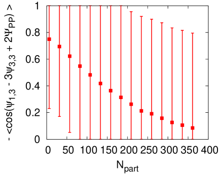
and illustrate the result in Fig. 6. We will use this correlation in Section V.1 to make a definite prediction for the behavior of two particle correlations with respect to the reaction plane.
Refer to caption
Figure 6: Correlation of the true dipole angle ψ1,3subscript𝜓13\psi_{1,3} and the estimated event plane angle ψ1,3mp=3ψ3,32ΨPPπsuperscriptsubscript𝜓13mp3subscript𝜓332subscriptΨ𝑃𝑃𝜋\psi_{1,3}^{\rm mp}=3\psi_{3,3}-2\Psi_{PP}-\pi. The points indicate the average cos(ψ1,3ψ1,3mp)delimited-⟨⟩delimited-⟨⟩subscript𝜓13superscriptsubscript𝜓13mp\langle\!\langle\cos(\psi_{1,3}-\psi_{1,3}^{\rm mp})\rangle\!\rangle and the errorbars indicate the variance of this quantity at fixed Npartsubscript𝑁partN_{\rm part}.

II.5 Convergence of the cumulant expansion for smooth Glauber type initial conditions

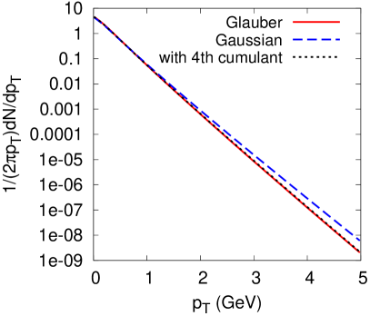
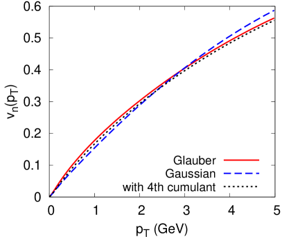
In the previous section we introduced a cumulant expansion to characterize the response of the system to a set of perturbations. In this section we will study the convergence of the cumulant expansion. Specifically, for a smooth (optical) Glauber profile, we will replace the initial entropy distribution with an approximately Gaussian profile and cumulant corrections through forth order. The distribution of entropy in the optical Glauber model (see Appendix A.2) is first used to calculate r2delimited-⟨⟩superscript𝑟2\left\langle r^{2}\right\rangle and r2cos2ϕdelimited-⟨⟩superscript𝑟22italic-ϕ\left\langle r^{2}\cos 2\phi\right\rangle, which determines the two coefficients of the Gaussian. Also the normalization (i.e. the total entropy) is the same between the Gaussian and the Glauber distribution. Taking the impact parameter to be b=7.6𝑏7.6b=7.6\,fm, Fig. 7 compares the spectra and the elliptic flow for these two distributions. In the next approximation, the fourth cumulants to the Gaussian are adjusted as described in Section II.4 and Appendix A.2 to reproduce the r4delimited-⟨⟩superscript𝑟4\left\langle r^{4}\right\rangle, r4cos2ϕdelimited-⟨⟩superscript𝑟42italic-ϕ\left\langle r^{4}\cos 2\phi\right\rangle, and r4cos4ϕdelimited-⟨⟩superscript𝑟44italic-ϕ\left\langle r^{4}\cos 4\phi\right\rangle moments of the Glauber distribution. Fig. 7 shows that the cumulant expansion reproduces the response of the Glauber distribution in detail.
Refer to caption
Refer to caption
Figure 7: (Color Online) (a) Spectra in the smooth (optical) Glauber model compared to the cumulant expansion. The coefficients of the Gaussian and fourth order cumulant expansions have been adjusted to reproduce r2delimited-⟨⟩superscript𝑟2\left\langle r^{2}\right\rangle, r2cos2ϕdelimited-⟨⟩superscript𝑟22italic-ϕ\left\langle r^{2}\cos 2\phi\right\rangle and r4cos2ϕdelimited-⟨⟩superscript𝑟42italic-ϕ\left\langle r^{4}\cos 2\phi\right\rangle, r4cos4ϕdelimited-⟨⟩superscript𝑟44italic-ϕ\left\langle r^{4}\cos 4\phi\right\rangle respectively. The total entropy of the cumulant expansion is also matched to the total entropy of the glauber distribution. (b) Elliptic flow in the Glauber model compared to the cumulant expansion.

III Time development of the response

In the previous sections we introduced a set of initial conditions with definite triangularity and dipole asymmetry. In this section we will show how the hydrodynamic response to these cumulants develops in space and time. The point here is to understand the hydrodynamics without the complications of freezeout and a freezeout prescription.

To show how the dipole and triangular flow develop in time, we have generalized the discussion of elliptic flow given in Ref. Kolb:2000sd . The spatial anisotropy is characterized by the second moment

ϵ2x=r2cos2ϕr2,subscriptitalic-ϵ2𝑥delimited-⟨⟩superscript𝑟22italic-ϕdelimited-⟨⟩superscript𝑟2\epsilon_{2x}=-\frac{\left\langle r^{2}\cos 2\phi\right\rangle}{\left\langle r^{2}\right\rangle}\,, (47)

which is a function of time in general. As the system expands, the spatial anisotropy decreases and the momentum anisotropy increases. The momentum anisotropy is traditionally defined with ϵ2psubscriptitalic-ϵ2𝑝\epsilon_{2p} :

ϵ2psubscriptitalic-ϵ2𝑝absent\displaystyle\epsilon_{2p}\equiv d2𝒙(TxxTyy)d2𝒙(Txx+Tyy)=d2𝒙(e+p)ur2cos2ϕud2𝒙[(e+p)ur2+2p],superscriptd2𝒙superscript𝑇𝑥𝑥superscript𝑇𝑦𝑦superscriptd2𝒙superscript𝑇𝑥𝑥superscript𝑇𝑦𝑦superscriptd2𝒙𝑒𝑝superscriptsubscript𝑢𝑟22subscriptitalic-ϕ𝑢superscriptd2𝒙delimited-[]𝑒𝑝superscriptsubscript𝑢𝑟22𝑝\displaystyle\frac{\int{\rm d}^{2}{\bm{x}}\,(T^{xx}-T^{yy})}{\int{\rm d}^{2}{\bm{x}}\,\left(T^{xx}+T^{yy}\right)}=\frac{\int{\rm d}^{2}{\bm{x}}\,(e+p)u_{r}^{2}\cos 2\phi_{u}}{\int{\rm d}^{2}{\bm{x}}\,\left[(e+p)u_{r}^{2}+2p\right]}\,, (48)

where ur=(ux)2+(uy)2subscript𝑢𝑟superscriptsuperscript𝑢𝑥2superscriptsuperscript𝑢𝑦2u_{r}=\sqrt{(u^{x})^{2}+(u^{y})^{2}} and ϕu=tan1(uy/ux)subscriptitalic-ϕ𝑢superscript1superscript𝑢𝑦superscript𝑢𝑥\phi_{u}=\tan^{-1}(u^{y}/u^{x}) . This definition has its flaws since the numerators and denominators do not transform as components of a tensor under transverse boosts111This flaw is easily remedied by replacing d2𝒙superscriptd2𝒙{\rm d}^{2}{\bm{x}} with the fluid three volume in the local rest frame dΣμuμ=d2𝒙dητu0𝑑subscriptΣ𝜇superscript𝑢𝜇superscriptd2𝒙d𝜂𝜏superscript𝑢0d\Sigma_{\mu}u^{\mu}={\rm d}^{2}{\bm{x}}{\rm d}\eta\,\tau u^{0}. The additional factor of u0superscript𝑢0u^{0} appears naturally below.Teaney:2009qa . An alternative definition is found by constructing an irreducible rank two tensor out of the momentum density T0isuperscript𝑇0𝑖T^{0i} and the flow velocity ujsuperscript𝑢𝑗u^{j}

T0(iuj)traces12(T0iuj+T0juiδijT0lul).T^{0(i}u^{j)}-\mbox{traces}\equiv\frac{1}{2}\left(T^{0i}u^{j}+T^{0j}u^{i}-\delta^{ij}T^{0l}u_{l}\right)\,. (49)

Then we define

ϵ2p=subscriptitalic-ϵ2𝑝absent\displaystyle\epsilon_{2p}= d2𝒙τ[T0(xux)traces]d2𝒙τ[T00u0]=d2𝒙τu0[(e+p)ur2cos2ϕu]d2𝒙τu0[(e+p)ur2+e],\displaystyle\frac{\int{\rm d}^{2}{\bm{x}}\tau\left[T^{0(x}u^{x)}-\mbox{traces}\right]}{\int{\rm d}^{2}{\bm{x}}\tau\left[T^{00}u^{0}\right]}=\frac{\int{\rm d}^{2}{\bm{x}}\,\tau u^{0}\left[(e+p)u_{r}^{2}\cos 2\phi_{u}\right]}{\int{\rm d}^{2}{\bm{x}}\,\tau u^{0}\left[(e+p)u_{r}^{2}+e\right]}\,, (50)

which is almost the same as Eq. (48). For the triangularity and dipole asymmetry we define the (reducible) third rank tensor

T0(iujul)=13!(T0iujul+perms).T^{0(i}u^{j}u^{l)}=\frac{1}{3!}\left(T^{0i}u^{j}u^{l}+\mbox{perms}\right)\,. (51)

Then the traceless (or irreducible) tensor is used to define the momentum space triangular anisotropy

ϵ3psubscriptitalic-ϵ3𝑝absent\displaystyle\epsilon_{3p}\equiv d2𝒙τ[T0(xuxux)traces]d2𝒙τ[T00u0u0]=d2𝒙τu0[(e+p)ur3cos3ϕu]d2𝒙τ[T00u0u0],\displaystyle\frac{\int{\rm d}^{2}{\bm{x}}\tau\left[T^{0(x}u^{x}u^{x)}-\mbox{traces}\right]}{\int{\rm d}^{2}{\bm{x}}\tau\left[T^{00}u^{0}u^{0}\right]}=\frac{\int{\rm d}^{2}{\bm{x}}\,\tau u^{0}\left[(e+p)u_{r}^{3}\cos 3\phi_{u}\right]}{\int{\rm d}^{2}{\bm{x}}\tau\left[T^{00}u^{0}u^{0}\right]}\,, (52)

and the trace is used to define momentum space dipole asymmetry

ϵ1psubscriptitalic-ϵ1𝑝absent\displaystyle\epsilon_{1p}\equiv d2𝒙τ[δjlT0(xujul)]d2𝒙τ[T00u0u0]=d2𝒙τu0[(e+p)ur3cosϕu]d2𝒙τ[T00u0u0].\displaystyle\frac{\int{\rm d}^{2}{\bm{x}}\tau\left[\delta_{jl}T^{0(x}u^{j}u^{l)}\right]}{\int{\rm d}^{2}{\bm{x}}\tau\left[T^{00}u^{0}u^{0}\right]}=\frac{\int{\rm d}^{2}{\bm{x}}\,\tau u^{0}\left[(e+p)u_{r}^{3}\cos\phi_{u}\right]}{\int{\rm d}^{2}{\bm{x}}\tau\left[T^{00}u^{0}u^{0}\right]}\,. (53)

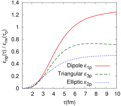
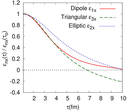
Armed with these definitions, Fig. 8 illustrates the
Refer to caption
Refer to caption
Figure 8: (Color online) (a) The spatial anisotropy of the entropy distribution ϵ1xsubscriptitalic-ϵ1𝑥\epsilon_{1x}, ϵ2xsubscriptitalic-ϵ2𝑥\epsilon_{2x}, and ϵ3xsubscriptitalic-ϵ3𝑥\epsilon_{3x} (see text) as a function of time for b=7.6fm𝑏7.6fmb=7.6\,{\rm fm}. (b) The momentum anisotropy ϵ1psubscriptitalic-ϵ1𝑝\epsilon_{1p}, ϵ2psubscriptitalic-ϵ2𝑝\epsilon_{2p}, and ϵ3psubscriptitalic-ϵ3𝑝\epsilon_{3p} (see text) as a function of time. The timescale in these figures should be compared to r2/cs5.4fmsimilar-to-or-equalsdelimited-⟨⟩superscript𝑟2subscript𝑐𝑠5.4fm\sqrt{\left\langle r^{2}\right\rangle}/c_{s}\simeq 5.4\,{\rm fm}.

development of the triangular flow and the dipole asymmetry as a function of time. As is familiar from studies of the elliptic flow Kolb:2000sd ; Ollitrault:1992bk , the spatial anisotropy decreases leading to a growth of the momentum space anisotropy. When the spatial anisotropy crosses zero, the growth of the momentum space anisotropy stalls. The figures also indicate that the elliptic flow, the dipole asymmetry, and the triangularity all develop on approximately the same time scale, τr2/cssimilar-to-or-equals𝜏delimited-⟨⟩superscript𝑟2subscript𝑐𝑠\tau\simeq\sqrt{\left\langle r^{2}\right\rangle}/c_{s}.

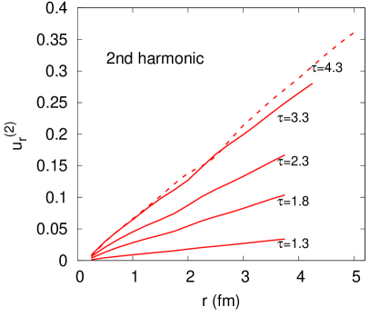
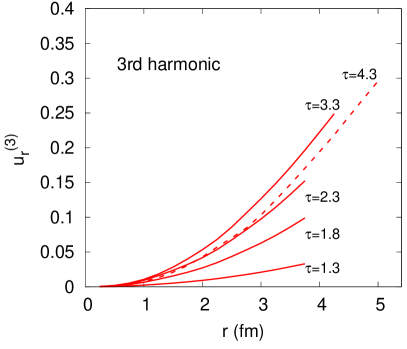
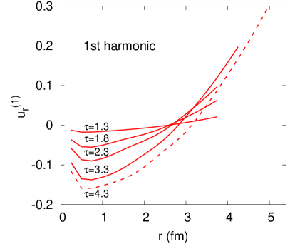
Another important aspect of the flow is the transverse radial flow profile. To illustrate this profile we decompose the transverse flow velocity into harmonics:

ur(r,ϕ)=subscript𝑢𝑟𝑟italic-ϕabsent\displaystyle u_{r}(r,\phi)= ur0(r)+2ur(1)(r)cos(ϕ)+2ur(2)(r)cos(2ϕ)+2ur(3)(r)cos(3ϕ)+.superscriptsubscript𝑢𝑟0𝑟2superscriptsubscript𝑢𝑟1𝑟italic-ϕ2superscriptsubscript𝑢𝑟2𝑟2italic-ϕ2superscriptsubscript𝑢𝑟3𝑟3italic-ϕ\displaystyle u_{r}^{0}(r)+2u_{r}^{(1)}(r)\cos(\phi)+2u_{r}^{(2)}(r)\cos(2\phi)+2u_{r}^{(3)}(r)\cos(3\phi)+\ldots\,. (54)

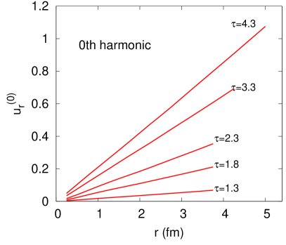
For a radially symmetric Gaussian distribution only the zero-th harmonic is present, and ur(0)superscriptsubscript𝑢𝑟0u_{r}^{(0)} shows a linearly rising flow profile. When the elliptic deformation is added the second harmonic also shows a linearly rising profile. Close to the origin this behavior can be understood with a linearized analysis of the acoustic waves. The flow velocity in an acoustic analysis is the gradient of a scalar function ΦΦ\Phi which can be expanded in harmonics:

Φ(r,ϕ)=Φ(0)(r)+2Φ(2)(r)cos2ϕ+.Φ𝑟italic-ϕsuperscriptΦ0𝑟2superscriptΦ2𝑟2italic-ϕ\Phi(r,\phi)=\Phi^{(0)}(r)+2\Phi^{(2)}(r)\cos 2\phi+\ldots\,. (55)

If Φ(r,ϕ)Φ𝑟italic-ϕ\Phi(r,\phi) is an analytic function of x𝑥x and y𝑦y, then Φ(2)superscriptΦ2\Phi^{(2)} must be quadratic for small r𝑟r. Consequently the gradient of this function, ur(2)(r)subscriptsuperscript𝑢2𝑟𝑟u^{(2)}_{r}(r), rises linearly at small r𝑟r. Similarly, the triangular deformation Φ(3)(r)superscriptΦ3𝑟\Phi^{(3)}(r) should be cubic at small r𝑟r and the flow profile ur(3)subscriptsuperscript𝑢3𝑟u^{(3)}_{r} should be quadratic. These features are borne out by our numerical work as exhibited in Fig. 9. Fig. 9 also shows the flow profile of the first harmonic which results from an initial dipole asymmetry. The first harmonic shows a negative slope at small r𝑟r followed by a quadratically rising profile at larger r𝑟r.

Refer to caption
Refer to caption
Refer to caption
Refer to caption
Figure 9: (a) The zeroth harmonic of the flow profile (see Eq. 54) for the radially symmetric Gaussian adopted in this work. The root mean square radius of the Gaussian is adjusted to reproduce an impact parameter of 7.6fm7.6fm7.6\,{\rm fm}. (b) The second harmonic of the flow profile for an elliptic perturbation. (c) The third harmonic of the flow profile for a triangular perturbation (d) The first harmonic of the flow profile for a distribution with a net dipole asymmetry. The deformations ϵ1,ϵ2subscriptitalic-ϵ1subscriptitalic-ϵ2\epsilon_{1},\epsilon_{2} and ϵ3subscriptitalic-ϵ3\epsilon_{3} are all set to 0.10.10.1.

As seen from Fig. 9, the triangular and dipolar flows are biased towards the edge of the nucleus. In the next section we will see that due to this bias v1subscript𝑣1v_{1} and v3subscript𝑣3v_{3} are more sensitive to the freezeout prescription than v2subscript𝑣2v_{2}.

IV Particle spectra: v1(pT)subscript𝑣1subscript𝑝𝑇v_{1}(p_{T}) and v3(pT)subscript𝑣3subscript𝑝𝑇v_{3}(p_{T})

Having illustrated the essential features of the hydrodynamic response, we will compute the particle spectra associated with these flows. As discussed above, the analysis is limited to a classical massless ideal gas. We will follow the time honored, but poorly motivated prescription of specifying a freezeout temperature or a freezeout entropy density. Freezeout temperatures in full hydrodynamic simulations with a Hadronic Resonance Gas (HRG) range from T=160MeV𝑇160MeVT=160\,{\rm MeV} to T=120MeV𝑇120MeVT=120\,{\rm MeV} Kolb:2003dz ; Teaney:2009qa . The total initial entropy and initial volume used in our massless ideal gas simulations were taken to be the similar to the total entropy and initial volume used in these full hydrodynamic simulations. The final freezeout volume of our massless-gas simulation is also taken to be similar to the final freezeout volume of these full simulations. Since entropy is conserved, this can be accomplished by adjusting the freezeout entropy density of the massless gas so that the entropy density equals the HRG entropy density for a specified HRG freezeout temperature. Experience has shown that this is a fair way to compare different equations of state. Rather than quoting the actual freezeout temperature of the massless gas EOS, we will simply quote the corresponding HRG freezeout temperature. Thus T170MeV𝑇170MeVT\Leftrightarrow 170\,{\rm MeV} means that the actual freezeout temperature is such that the entropy density of a massless gas is equal to the entropy density of the HRG at T=170MeV𝑇170MeVT=170\,{\rm MeV}. Table 1 shows a set of temperatures and entropy densities in a HRG model and the corresponding freezeout temperatures for the massless gas equation of state.

Hadron Gas Tfosubscript𝑇foT_{\rm fo} Hadron Gas sfosubscript𝑠fos_{\rm fo} Massless Gas Tfosubscript𝑇foT_{\rm fo}
130MeV130MeV130\,{\rm MeV} 4.34fm34.34superscriptfm34.34\,{\rm fm}^{-3} 71   MeV
150MeV150MeV150\,{\rm MeV} 1.87fm31.87superscriptfm31.87\,{\rm fm}^{-3} 96   MeV
170MeV170MeV170\,{\rm MeV} 0.77fm30.77superscriptfm30.77\,{\rm fm}^{-3} 127  MeV
Table 1: Table of freezeout temperatures used in this work. The first two columns show freezeout temperatures and the corresponding entropy densities of a Hadron Resonance Gas (HRG) EOS. The last column shows the freezeout temperatures where the massless gas EOS used in this work attains the corresponding HRG entropy density.

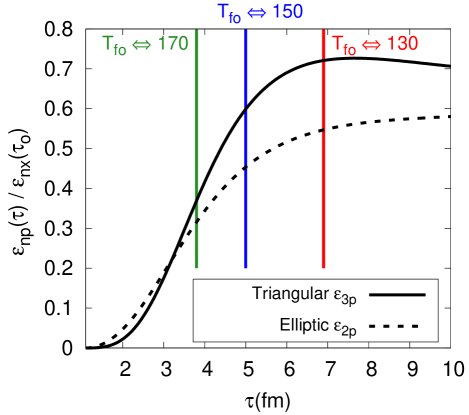
Fig. 10 shows the momentum anisotropies as a function of time, and marks when the average entropy density of the system reaches a specified freezeout entropy density. Specifically, the lines indicate when sdelimited-⟨⟩𝑠\left\langle s\right\rangle in the notation of Eq. (6) falls below the freezeout entropy density indicated in Table  1. We see that for Tfo170MeVsubscript𝑇fo170MeVT_{\rm fo}\Leftrightarrow 170\,{\rm MeV} the triangular and dipole flows are still developing, while for Tfo130MeVsubscript𝑇fo130MeVT_{\rm fo}\Leftrightarrow 130\,{\rm MeV} the flows are almost fully developed.

Refer to caption
Figure 10: Evolution of the momentum anisotropy as a function of time at an impact parameter of b=7.6fm𝑏7.6fmb=7.6\,{\rm fm}. The lines indicate when the average entropy density sdelimited-⟨⟩𝑠\left\langle s\right\rangle falls below the freezeout entropy density specified by the the temperatures T130,150,170MeV𝑇130150170MeVT\Leftrightarrow 130,150,170\,{\rm MeV}.

Once the freezeout surface is specified the particle spectra are computed using the Cooper-Frye formula

(2π)3EdNd3𝒑=Vpμ𝑑Vμfo(PU(X)),superscript2𝜋3𝐸𝑑𝑁superscript𝑑3𝒑subscript𝑉superscript𝑝𝜇differential-dsubscript𝑉𝜇subscript𝑓𝑜𝑃𝑈𝑋(2\pi)^{3}E\frac{dN}{d^{3}{\bm{p}}}=\int_{V}p^{\mu}dV_{\mu}\,f_{o}(-P\cdot U(X))\,, (56)

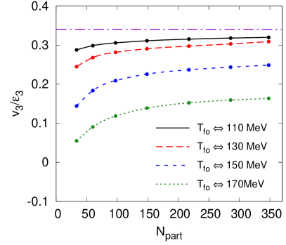
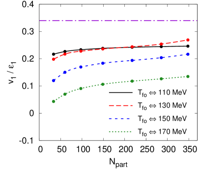
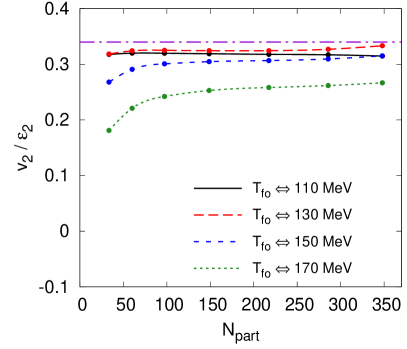
where fo(E)=gexp(E/T(X))subscript𝑓𝑜𝐸𝑔𝐸𝑇𝑋f_{o}(E)=g\exp(-E/T(X)) is the distribution function of a classical massless gas. (The notation here follows the review article Teaney:2009qa .) Using this formula we compute the particle spectra and determine the associated harmonics v1subscript𝑣1v_{1}, v2subscript𝑣2v_{2} and v3subscript𝑣3v_{3}. For each impact parameter we determine the root-mean square radius and the total entropy from an optical Glauber model; then the Gaussian parameters are adjusted to reproduce these Glauber quantities; finally the simulation is run to the freezeout entropy density and the harmonics are computed. Fig. 11 shows how the harmonics depend on centrality and the freezeout temperature.

Examining Fig. 11 we see that v1subscript𝑣1v_{1}, v2subscript𝑣2v_{2} and v3subscript𝑣3v_{3} are roughly independent of centrality. However, it must be borne in mind that in a more complete simulation, the total entropy per participant is also a function of centrality and this could change the result. Here the entropy per participant is constant. Generally the freezeout criterion is also a function of centrality and this could give a substantial shape to these curves in a final simulation. Finally, when viscosity is included the triangularity is also a more complicated function of centrality Alver:2010dn . This will be explored elsewhere YanWork .
Refer to caption
Refer to caption
Refer to caption
Figure 11: v1subscript𝑣1v_{1}, v2subscript𝑣2v_{2} and v3subscript𝑣3v_{3} per unit anisotropy as a function of Npartsubscript𝑁partN_{\rm part} for different freezeout temperatures. The anisotropy parameters are all 0.10.10.1 in the actual simulations.

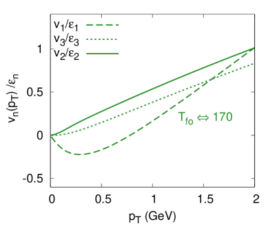
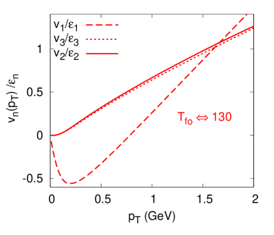
Fig. 12 shows how these harmonics depend on pTsubscript𝑝𝑇p_{T}. v2(pT)subscript𝑣2subscript𝑝𝑇v_{2}(p_{T}) and v3(pT)subscript𝑣3subscript𝑝𝑇v_{3}(p_{T}) show a characteristic linear rise with pTsubscript𝑝𝑇p_{T} that is a consequence of a strong radial flow Huovinen:2001cy ; Borghini:2005kd ; Mishra:2007tw ; Mishra:2008dm . Indeed examining the thermal distribution with constant temperature, we have

ePU/T=superscript𝑒𝑃𝑈𝑇absent\displaystyle e^{P\cdot U/T}= eE𝒑Uτ/TepT/Tur(r,ϕ)cos(ϕpϕu),superscript𝑒subscript𝐸𝒑superscript𝑈𝜏𝑇superscript𝑒subscript𝑝𝑇𝑇subscript𝑢𝑟𝑟italic-ϕsubscriptitalic-ϕ𝑝subscriptitalic-ϕ𝑢\displaystyle e^{-E_{\bm{p}}U^{\tau}/T}e^{p_{T}/T\,u_{r}(r,\phi)\cos(\phi_{p}-\phi_{u})}\,, (57)
similar-to-or-equals\displaystyle\simeq eE𝒑/TepT/Tur(0)(r)cos(ϕpϕ)superscript𝑒subscript𝐸𝒑𝑇superscript𝑒subscript𝑝𝑇𝑇superscriptsubscript𝑢𝑟0𝑟subscriptitalic-ϕ𝑝italic-ϕ\displaystyle e^{-E_{\bm{p}}/T}e^{p_{T}/Tu_{r}^{(0)}(r)\cos(\phi_{p}-\phi)}
×[1+2pTTur(2)(r)cos(2ϕ)cos(ϕ𝒑ϕ)+2pTTur(3)(r)cos(3ϕ)cos(ϕ𝒑ϕ)+].absentdelimited-[]12subscript𝑝𝑇𝑇superscriptsubscript𝑢𝑟2𝑟2italic-ϕsubscriptitalic-ϕ𝒑italic-ϕ2subscript𝑝𝑇𝑇superscriptsubscript𝑢𝑟3𝑟3italic-ϕsubscriptitalic-ϕ𝒑italic-ϕ\displaystyle\quad\times\left[1+\frac{2p_{T}}{T}u_{r}^{(2)}(r)\cos(2\phi)\cos(\phi_{\bm{p}}-\phi)+\frac{2p_{T}}{T}u_{r}^{(3)}(r)\cos(3\phi)\cos(\phi_{\bm{p}}-\phi)+\ldots\right]\,. (58)

Here E𝒑subscript𝐸𝒑E_{{\bm{p}}} is the energy, ϕ𝒑subscriptitalic-ϕ𝒑\phi_{{\bm{p}}} is the particles azimuthal angle; we have adopted a non-relativistic approximation Uτ1similar-to-or-equalssuperscript𝑈𝜏1U^{\tau}\simeq 1 and assumed that the flow is approximately radial, ϕuϕsimilar-to-or-equalssubscriptitalic-ϕ𝑢italic-ϕ\phi_{u}\simeq\phi. Further, we have neglected ur(1)superscriptsubscript𝑢𝑟1u_{r}^{(1)} in this discussion. Unless the momentum angle equals the spatial angle ϕ𝒑ϕsimilar-to-or-equalssubscriptitalic-ϕ𝒑italic-ϕ\phi_{\bm{p}}\simeq\phi, the thermal distribution is strongly suppressed by the leading Boltzmann factor. Thus, we arrive at a form which illustrates the linear rise of rise of vn(pT)subscript𝑣𝑛subscript𝑝𝑇v_{n}(p_{T}) with pTsubscript𝑝𝑇p_{T}

ePU/Tsimilar-to-or-equalssuperscript𝑒𝑃𝑈𝑇absent\displaystyle e^{P\cdot U/T}\simeq eE𝒑/TepT/Tur(0)(r)[1+2pTTur(2)(r)cos(2ϕ𝒑)+2pTTur(3)(r)cos(3ϕ𝒑)+].superscript𝑒subscript𝐸𝒑𝑇superscript𝑒subscript𝑝𝑇𝑇superscriptsubscript𝑢𝑟0𝑟delimited-[]12subscript𝑝𝑇𝑇superscriptsubscript𝑢𝑟2𝑟2subscriptitalic-ϕ𝒑2subscript𝑝𝑇𝑇superscriptsubscript𝑢𝑟3𝑟3subscriptitalic-ϕ𝒑\displaystyle e^{-E_{\bm{p}}/T}e^{p_{T}/Tu_{r}^{(0)}(r)}\left[1+\frac{2p_{T}}{T}u_{r}^{(2)}(r)\cos(2\phi_{\bm{p}})+\frac{2p_{T}}{T}u_{r}^{(3)}(r)\cos(3\phi_{\bm{p}})+\ldots\right]\,. (59)

Examining Fig. 12, we see that v1(pT)subscript𝑣1subscript𝑝𝑇v_{1}(p_{T}) also displays a similar linearly rising trend at higher pTsubscript𝑝𝑇p_{T} after an initial dip.

Refer to caption
Refer to caption
Figure 12: vn(pT)subscript𝑣𝑛subscript𝑝𝑇v_{n}(p_{T}) for two different freezeout temperatures as described in Table 1. The root mean square radius of the initial Gaussian corresponds to a radius of b=7.6fm𝑏7.6fmb=7.6\,{\rm fm}

V Further predictions and comparison with other works.

V.1 Further predictions

Fig. 11 and Fig. 12 show the response of the hydrodynamic system to the deformations. Certainly it is premature to compare the current calculation to data. For instance, the effect of viscosity, resonance decays, and a lattice-based equation of state have not been included. These reality factors will reduce the response. Nevertheless, in order to keep the final goal clearly in sight, we will provisionally compare the current calculation to the Alver Roland fit Alver:2010gr of STAR inclusive two particle correlations Abelev:2008un . Further, we will suggest a number of additional observables which can confirm the geometric nature of the measured two particle correlations.

The average over glauber configurations at fixed Npartsubscript𝑁partN_{\rm part} is denoted with double brackets delimited-⟨⟩delimited-⟨⟩\langle\!\langle\ldots\rangle\!\rangle. Then the two particle angular correlation function can be expanded in a Fourier series:

dNpairs,αβdϕαdϕβ=Npairs,αβ(1+n2VnΔcos(nϕαnϕβ)).delimited-⟨⟩delimited-⟨⟩dsubscript𝑁pairs𝛼𝛽dsubscriptitalic-ϕ𝛼dsubscriptitalic-ϕ𝛽delimited-⟨⟩delimited-⟨⟩subscript𝑁pairs𝛼𝛽1subscript𝑛2subscript𝑉𝑛Δ𝑛subscriptitalic-ϕ𝛼𝑛subscriptitalic-ϕ𝛽\displaystyle\left\langle\!\!\left\langle\frac{{\rm d}N_{\rm pairs,\alpha\beta}}{{\rm d}\phi_{\alpha}{\rm d}\phi_{\beta}}\right\rangle\!\!\right\rangle=\langle\!\langle N_{\rm pairs,\alpha\beta}\rangle\!\rangle\left(1+\sum_{n}2V_{n\Delta}\cos(n\phi_{\alpha}-n\phi_{\beta})\right)\,. (60)

The particle labels α𝛼\alpha and β𝛽\beta could denote distinct particle types or pTsubscript𝑝𝑇p_{T} bins for example. Following Alver and Roland we will approximate the two particle correlation with the disconnected component. The yield of particle type α𝛼\alpha for a fixed Glauber configuration is

dNαdϕα=Nα2π[1+2v1αϵ1ϵ1cos(ϕαψ1,3)+2v2αϵ2ϵ2cos(2ϕα2ΨPP)+2v3αϵ3ϵ3cos(3ϕα3ψ3,3)],dsubscript𝑁𝛼dsubscriptitalic-ϕ𝛼subscript𝑁𝛼2𝜋delimited-[]12subscript𝑣1𝛼subscriptitalic-ϵ1subscriptitalic-ϵ1subscriptitalic-ϕ𝛼subscript𝜓132subscript𝑣2𝛼subscriptitalic-ϵ2subscriptitalic-ϵ22subscriptitalic-ϕ𝛼2subscriptΨ𝑃𝑃2subscript𝑣3𝛼subscriptitalic-ϵ3subscriptitalic-ϵ33subscriptitalic-ϕ𝛼3subscript𝜓33\frac{{\rm d}N_{\alpha}}{{\rm d}\phi_{\alpha}}=\frac{N_{\alpha}}{2\pi}\Big{[}1+2\frac{v_{1\alpha}}{\epsilon_{1}}\epsilon_{1}\cos(\phi_{\alpha}-\psi_{1,3})+2\frac{v_{2\alpha}}{\epsilon_{2}}\epsilon_{2}\cos(2\phi_{\alpha}-2\Psi_{PP})\\ +2\frac{v_{3\alpha}}{\epsilon_{3}}\epsilon_{3}\cos(3\phi_{\alpha}-3\psi_{3,3})\Big{]}\,, (61)

where we have assumed that the response is linearly proportional to the deformation. Then the two particle correlation function is approximated as

dNpairs,αβdϕαdϕβdNdϕαdNdϕβNαNβ(2π)2[1+n2(vnαvnβϵn2)ϵn2cos(n(ϕαϕβ))].similar-to-or-equalsdelimited-⟨⟩delimited-⟨⟩dsubscript𝑁pairs𝛼𝛽dsubscriptitalic-ϕ𝛼dsubscriptitalic-ϕ𝛽delimited-⟨⟩delimited-⟨⟩d𝑁dsubscriptitalic-ϕ𝛼d𝑁dsubscriptitalic-ϕ𝛽similar-to-or-equalssubscript𝑁𝛼subscript𝑁𝛽superscript2𝜋2delimited-[]1subscript𝑛2subscript𝑣𝑛𝛼subscript𝑣𝑛𝛽superscriptsubscriptitalic-ϵ𝑛2delimited-⟨⟩delimited-⟨⟩superscriptsubscriptitalic-ϵ𝑛2𝑛subscriptitalic-ϕ𝛼subscriptitalic-ϕ𝛽\left\langle\!\!\left\langle\frac{{\rm d}N_{\rm pairs,\alpha\beta}}{{\rm d}\phi_{\alpha}{\rm d}\phi_{\beta}}\right\rangle\!\!\right\rangle\simeq\left\langle\!\!\left\langle\frac{{\rm d}N}{{\rm d}\phi_{\alpha}}\frac{{\rm d}N}{{\rm d}\phi_{\beta}}\right\rangle\!\!\right\rangle\simeq\frac{N_{\alpha}N_{\beta}}{(2\pi)^{2}}\left[1+\sum_{n}2\left(\frac{v_{n\alpha}v_{n\beta}}{\epsilon_{n}^{2}}\right)\langle\!\langle\epsilon_{n}^{2}\rangle\!\rangle\cos(n(\phi_{\alpha}-\phi_{\beta}))\right]\,. (62)

Here and below we have tacitly assumed that the multiplicity fluctuations at fixed Npartsubscript𝑁partN_{\rm part} are negligible. If this is not the case then one has the following replacements in Eq. (62)

NαNβNαNβϵn2NαNβϵn2NαNβ.formulae-sequencesubscript𝑁𝛼subscript𝑁𝛽delimited-⟨⟩delimited-⟨⟩subscript𝑁𝛼subscript𝑁𝛽delimited-⟨⟩delimited-⟨⟩superscriptsubscriptitalic-ϵ𝑛2delimited-⟨⟩delimited-⟨⟩subscript𝑁𝛼subscript𝑁𝛽superscriptsubscriptitalic-ϵ𝑛2delimited-⟨⟩delimited-⟨⟩subscript𝑁𝛼subscript𝑁𝛽N_{\alpha}N_{\beta}\rightarrow\langle\!\langle N_{\alpha}N_{\beta}\rangle\!\rangle\qquad\langle\!\langle\epsilon_{n}^{2}\rangle\!\rangle\rightarrow\frac{\langle\!\langle N_{\alpha}N_{\beta}\epsilon_{n}^{2}\rangle\!\rangle}{\langle\!\langle N_{\alpha}N_{\beta}\rangle\!\rangle}\,. (63)

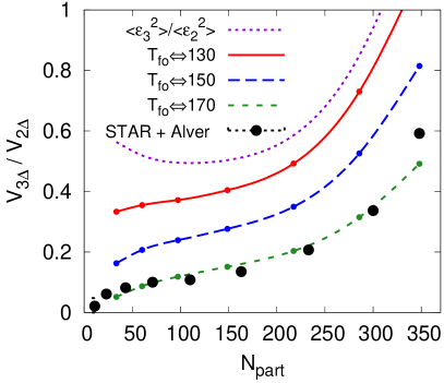
Given the parameterizations in Eq. (60) and Eq. (62), the response functions in Fig. 11 make a definite prediction for the different Fourier components VnΔsubscript𝑉𝑛ΔV_{n\Delta}. The elliptic flow is too large in the ideal massless gas model considered here. We will therefore simply plot the ratios of the different fourier components as was done in the Alver and Roland paper. Using the response functions in Fig. 11, and the Glauber estimates for ϵ32/ϵ22delimited-⟨⟩delimited-⟨⟩superscriptsubscriptitalic-ϵ32delimited-⟨⟩delimited-⟨⟩superscriptsubscriptitalic-ϵ22\langle\!\langle\epsilon_{3}^{2}\rangle\!\rangle/\langle\!\langle\epsilon_{2}^{2}\rangle\!\rangle, Fig. 13(a) compares the strength of the triangular component to the quadrapole component.
Refer to caption
Refer to caption
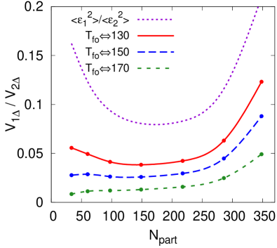
Figure 13: Fourier components of the two particle correlation function as a function of Npartsubscript𝑁partN_{\rm part} relative to the quadrapole component. (a) The triangularity component compared to the Alver Roland fit Alver:2010gr of STAR inclusive two particle correlation functions Abelev:2008un . (b) The dipole component relative to the quadrapole component; note that the scales differ between(a) and(b).

The ideal hydrodynamic prediction (with a massless ideal gas EOS) is generally too large and fairly sensitive to the freezeout temperature. This sensitivity reflects the fact that the triangular flow develops further towards the edge of the nucleus. Fig. 13(b) compares the dipole component to the quadrapole component. The dipole component is a factor of eight smaller than the quadrapole component. This is a reflection of the fact that ϵ1subscriptitalic-ϵ1\epsilon_{1} is small, and the fact that v1(pT)/ϵ1subscript𝑣1subscript𝑝𝑇subscriptitalic-ϵ1v_{1}(p_{T})/\epsilon_{1} is positive and negative. The dipolar flow is also sensitive to the details of freezeout.
Next we wish to determine the general form of the two particle correlation function with respect to the participant plane ΨPPsubscriptΨ𝑃𝑃\Psi_{PP}

dNpairs,αβdϕ1dϕ2ΨPPdNαd(ϕαΨPP)dNβd(ϕβΨPP)ΨPP.similar-to-or-equalssubscriptdelimited-⟨⟩delimited-⟨⟩dsubscript𝑁pairs𝛼𝛽dsubscriptitalic-ϕ1dsubscriptitalic-ϕ2subscriptΨ𝑃𝑃subscriptdelimited-⟨⟩delimited-⟨⟩dsubscript𝑁𝛼dsubscriptitalic-ϕ𝛼subscriptΨ𝑃𝑃dsubscript𝑁𝛽dsubscriptitalic-ϕ𝛽subscriptΨ𝑃𝑃subscriptΨ𝑃𝑃\left\langle\!\!\left\langle\frac{{\rm d}N_{\rm pairs,\alpha\beta}}{{\rm d}\phi_{1}{\rm d}\phi_{2}}\right\rangle\!\!\right\rangle_{\Psi_{PP}}\simeq\left\langle\!\!\left\langle\frac{{\rm d}N_{\alpha}}{{\rm d}(\phi_{\alpha}-\Psi_{PP})}\frac{{\rm d}N_{\beta}}{{\rm d}(\phi_{\beta}-\Psi_{PP})}\right\rangle\!\!\right\rangle_{\Psi_{PP}}\,.\\ (64)

Inserting Eq. (61) into Eq. (64) and averaging over glauber configurations several several terms appear. In Section B we identified the principle correlations that exist between the angles ψ1,3,ψ3,3subscript𝜓13subscript𝜓33\psi_{1,3},\psi_{3,3} and ΨPPsubscriptΨ𝑃𝑃\Psi_{PP}. Namely, the only significant fourier expectation values are cos(2ψ1,32ΨPP)delimited-⟨⟩2subscript𝜓132subscriptΨ𝑃𝑃\left\langle\cos(2\psi_{1,3}-2\Psi_{PP})\right\rangle (as determined by the coefficient A𝐴A in Eq. (36)), and cos(ψ1,33ψ3,3+2ΨPP)delimited-⟨⟩subscript𝜓133subscript𝜓332subscriptΨ𝑃𝑃\left\langle\cos(\psi_{1,3}-3\psi_{3,3}+2\Psi_{PP})\right\rangle (as determined by the coefficient B0subscript𝐵0B_{0} in Eq. (43)). With the assumption that these are the only significant fourier expectation values at third order, the form of the two particle correlation function with respect to participant plane becomes:

dNpairs,αβdϕαdϕβNαNβ(2π)2[1+\displaystyle\left\langle\!\!\left\langle\frac{{\rm d}N_{\rm pairs,\alpha\beta}}{{\rm d}\phi_{\alpha}{\rm d}\phi_{\beta}}\right\rangle\!\!\right\rangle\simeq\frac{N_{\alpha}N_{\beta}}{(2\pi)^{2}}\Big{[}1+ n2(vnαvnβϵn2)ϵn2cos(nϕαnϕβ)subscript𝑛2subscript𝑣𝑛𝛼subscript𝑣𝑛𝛽superscriptsubscriptitalic-ϵ𝑛2delimited-⟨⟩delimited-⟨⟩superscriptsubscriptitalic-ϵ𝑛2𝑛subscriptitalic-ϕ𝛼𝑛subscriptitalic-ϕ𝛽\displaystyle\sum_{n}2\left(\frac{v_{n\alpha}v_{n\beta}}{\epsilon_{n}^{2}}\right)\langle\!\langle\epsilon_{n}^{2}\rangle\!\rangle\cos(n\phi_{\alpha}-n\phi_{\beta})
+\displaystyle+   2v2αϵ2ϵ2cos(2ϕα2ΨPP)2subscript𝑣2𝛼subscriptitalic-ϵ2delimited-⟨⟩delimited-⟨⟩subscriptitalic-ϵ22subscriptitalic-ϕ𝛼2subscriptΨ𝑃𝑃\displaystyle\,\,2\frac{v_{2\alpha}}{\epsilon_{2}}\langle\!\langle\epsilon_{2}\rangle\!\rangle\;\cos(2\phi_{\alpha}-2\Psi_{PP})
+\displaystyle+   2v2αv2βϵ22ϵ22cos(2ϕα+2ϕβ4ΨPP)2subscript𝑣2𝛼subscript𝑣2𝛽superscriptsubscriptitalic-ϵ22delimited-⟨⟩delimited-⟨⟩superscriptsubscriptitalic-ϵ222subscriptitalic-ϕ𝛼2subscriptitalic-ϕ𝛽4subscriptΨ𝑃𝑃\displaystyle\,\,2\frac{v_{2\alpha}v_{2\beta}}{\epsilon_{2}^{2}}\langle\!\langle\epsilon_{2}^{2}\rangle\!\rangle\;\cos(2\phi_{\alpha}+2\phi_{\beta}-4\Psi_{PP})
+\displaystyle+    2v1αv1βϵ12ϵ12cos(2ψ1,32ΨPP)cos(ϕα+ϕβ2ΨPP)2subscript𝑣1𝛼subscript𝑣1𝛽superscriptsubscriptitalic-ϵ12delimited-⟨⟩delimited-⟨⟩superscriptsubscriptitalic-ϵ122subscript𝜓132subscriptΨ𝑃𝑃subscriptitalic-ϕ𝛼subscriptitalic-ϕ𝛽2subscriptΨ𝑃𝑃\displaystyle\,\,\,2\frac{v_{1\alpha}v_{1\beta}}{\epsilon_{1}^{2}}\langle\!\langle\epsilon_{1}^{2}\cos(2\psi_{1,3}-2\Psi_{PP})\rangle\!\rangle\;\cos(\phi_{\alpha}+\phi_{\beta}-2\Psi_{PP})
+\displaystyle+   2v1αv3βϵ1ϵ3ϵ1ϵ3cos(ψ1,33ψ3,3+2ΨPP)cos(ϕα3ϕβ+2ΨPP)2subscript𝑣1𝛼subscript𝑣3𝛽subscriptitalic-ϵ1subscriptitalic-ϵ3delimited-⟨⟩delimited-⟨⟩subscriptitalic-ϵ1subscriptitalic-ϵ3subscript𝜓133subscript𝜓332subscriptΨ𝑃𝑃subscriptitalic-ϕ𝛼3subscriptitalic-ϕ𝛽2subscriptΨ𝑃𝑃\displaystyle\,\,2\frac{v_{1\alpha}v_{3\beta}}{\epsilon_{1}\epsilon_{3}}\langle\!\langle\epsilon_{1}\epsilon_{3}\cos(\psi_{1,3}-3\psi_{3,3}+2\Psi_{PP})\rangle\!\rangle\cos(\phi_{\alpha}-3\phi_{\beta}+2\Psi_{PP})
+\displaystyle+ αβ].\displaystyle\,\,\alpha\leftrightarrow\beta\Big{]}\,. (65)

The symmetrization with respect to α𝛼\alpha and β𝛽\beta applies to all terms in this expression which are not already symmetric, e.g. cos(2ϕα2ΨPP)2subscriptitalic-ϕ𝛼2subscriptΨ𝑃𝑃\cos(2\phi_{\alpha}-2\Psi_{PP}). We will discuss this expression line by line. The first three lines are not particularly novel: The first line is independent of the reaction plane angle ΨPPsubscriptΨ𝑃𝑃\Psi_{PP}. The next two lines reflect the underlying elliptic flow and would normally be subtracted in a flow subtracted two particle correlation function.

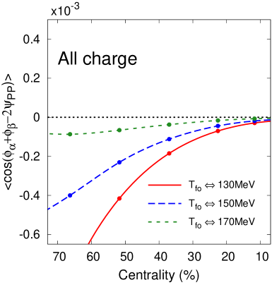
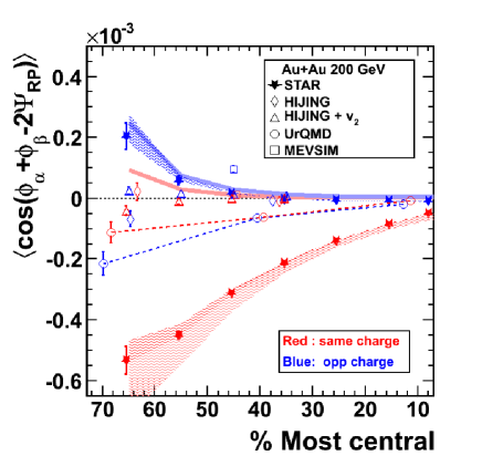
The fourth line contains the first novel feature. This term arises because the dipole asymmetry is preferentially oriented out plane, leading to a net v1subscript𝑣1v_{1} out of plane. Fig. 14(a) shows the correlation function cos(ϕα+ϕβ2ΨPP)delimited-⟨⟩subscriptitalic-ϕ𝛼subscriptitalic-ϕ𝛽2subscriptΨ𝑃𝑃\left\langle\cos(\phi_{\alpha}+\phi_{\beta}-2\Psi_{PP})\right\rangle as a function of centrality. Recently, the STAR collaboration measured a similar expectation value, but divided correlation function into the different possible charge components (i.e.formulae-sequence𝑖𝑒i.e.++, +-, –) in order to investigate the possibility of local parity violation in heavy ion collisions Abelev:2009uh ; Abelev:2009txa ; Kharzeev:1998kz . Fig. 14(b) shows the measured STAR correlations. The measured correlation is the same order of magnitude as the out of plane flow found in this work. However many aspects of the out of plane dipole flow (e.g. the pTsubscript𝑝𝑇p_{T} dependence and most importantly the charge dependence) do not agree with the measured correlation. Thus the STAR measurements can constraint the geometric fluctuations reported here. This will be investigated in future work.
Refer to caption
Refer to caption
Figure 14: (a) The expectation value cos(ϕα+ϕβ2ΨPP)delimited-⟨⟩subscriptitalic-ϕ𝛼subscriptitalic-ϕ𝛽2subscriptΨ𝑃𝑃\left\langle\cos(\phi_{\alpha}+\phi_{\beta}-2\Psi_{PP})\right\rangle as predicted by hydrodynamics, where α𝛼\alpha and β𝛽\beta label all particles. (b) The charge asymmetry with respect to reaction plane cos(ϕα+ϕβ2ΨR)delimited-⟨⟩subscriptitalic-ϕ𝛼subscriptitalic-ϕ𝛽2subscriptΨ𝑅\left\langle\cos(\phi_{\alpha}+\phi_{\beta}-2\Psi_{R})\right\rangle as measured by the STAR collaboration Abelev:2009uh ; Abelev:2009txa . Here α𝛼\alpha and β𝛽\beta label ++,+,++,+-, or --. The hydrodynamic prediction does not explain the charge asymmetry.

A second novel feature expressed by the two particle correlation function with respect to reaction plane is recorded by the 5th line of Eq. (64). It shows that hydrodynamics, together with the geometric fluctuations of the Glauber model makes a definite prediction for the angular correlation

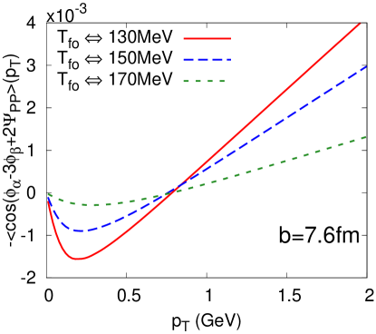
cos(ϕα3ϕβ+2ΨPP).delimited-⟨⟩delimited-⟨⟩subscriptitalic-ϕ𝛼3subscriptitalic-ϕ𝛽2subscriptΨ𝑃𝑃\langle\!\langle\cos(\phi_{\alpha}-3\phi_{\beta}+2\Psi_{PP})\rangle\!\rangle\,. (66)

Taking α𝛼\alpha to label all the particles in a definite pTsubscript𝑝𝑇p_{T} bin and β𝛽\beta all the particles, this definite prediction reads

cos(ϕα3ϕβ+2ΨPP)=v1(pT)ϵ1v3ϵ3ϵ1ϵ3cos(ψ1,33ψ3,3+2ΨPP).delimited-⟨⟩delimited-⟨⟩subscriptitalic-ϕ𝛼3subscriptitalic-ϕ𝛽2subscriptΨ𝑃𝑃subscript𝑣1subscript𝑝𝑇subscriptitalic-ϵ1subscript𝑣3subscriptitalic-ϵ3delimited-⟨⟩delimited-⟨⟩subscriptitalic-ϵ1subscriptitalic-ϵ3subscript𝜓133subscript𝜓332subscriptΨ𝑃𝑃\langle\!\langle\cos(\phi_{\alpha}-3\phi_{\beta}+2\Psi_{PP})\rangle\!\rangle=\frac{v_{1}(p_{T})}{\epsilon_{1}}\frac{v_{3}}{\epsilon_{3}}\langle\!\langle\epsilon_{1}\epsilon_{3}\cos(\psi_{1,3}-3\psi_{3,3}+2\Psi_{PP})\rangle\!\rangle\,. (67)

This result is illustrated in Fig. 15 and is based on the Glauber analysis in Fig. 6 and the response functions calculated in Fig. 12. Another way to probe this same correlation is the following. Experimentally, the participant plane ΨPPsubscriptΨ𝑃𝑃\Psi_{PP} is traditionally estimated by using the standard Q𝑄Q vector method, or the Yang-Lee zero generalization of this idea Voloshin:2008dg . These same methods can be used to determine the triangularity event plane ψ3,3subscript𝜓33\psi_{3,3} without significant modifications Voloshin_private . The strong correlation between the dipole, triangular, and participant planes implies that the knowledge of ψ3,3subscript𝜓33\psi_{3,3} and ΨPPsubscriptΨ𝑃𝑃\Psi_{PP} determines the dipole event plane ψ1,3subscript𝜓13\psi_{1,3} at least statistically. The most probable orientation is given by Eq. (45) and is repeated here for convenience

ψ1,3mp=3ψ3,32ΨPPπ.superscriptsubscript𝜓13mp3subscript𝜓332subscriptΨ𝑃𝑃𝜋\psi_{1,3}^{\rm mp}=3\psi_{3,3}-2\Psi_{PP}-\pi\,.

Thus, the v1subscript𝑣1v_{1} associated with the dipole asymmetry can be determined by measuring the expectation value

cos(ϕψ1,3mp).delimited-⟨⟩delimited-⟨⟩italic-ϕsuperscriptsubscript𝜓13mp\langle\!\langle\cos(\phi-\psi_{1,3}^{\rm mp})\rangle\!\rangle\,. (68)

Essentially this correlation is a v1subscript𝑣1v_{1} with an extra twist to take out the shifting orientations of the dipole and triangular event planes – see Fig. 5.
Refer to caption
Figure 15: A hydrodynamic prediction for the expectation value cos(ϕα3ϕβ+2ΨPP)delimited-⟨⟩subscriptitalic-ϕ𝛼3subscriptitalic-ϕ𝛽2subscriptΨ𝑃𝑃\left\langle\cos(\phi_{\alpha}-3\phi_{\beta}+2\Psi_{PP})\right\rangle which reflects the correlation between the dipole, triangular, and elliptic event planes. Here α𝛼\alpha labels all particles in a given pTsubscript𝑝𝑇p_{T} bin and β𝛽\beta labels all particles.

V.2 Discussion and comparison with other works

We hope that the cumulant expansion presented in Section II organizes and formalizes the study of fluctuations in heavy ion collisions. The convergence of the cumulant expansion is really quite good as illustrated in Fig. 7. At third order in the cumulant expansion there are two additional terms, the triangularity r3cos3(ϕψ3,3)delimited-⟨⟩superscript𝑟33italic-ϕsubscript𝜓33\left\langle r^{3}\cos 3(\phi-\psi_{3,3})\right\rangle, and the dipole asymmetry r3cos(ϕψ1,3)delimited-⟨⟩superscript𝑟3italic-ϕsubscript𝜓13\left\langle r^{3}\cos(\phi-\psi_{1,3})\right\rangle.

Our numerical results for the triangularity v3/ϵ3subscript𝑣3subscriptitalic-ϵ3v_{3}/\epsilon_{3} are similar to recently reported results Alver:2010dn ; Schenke:2010rr . However, v3subscript𝑣3v_{3} (and v1subscript𝑣1v_{1}) is significantly more sensitive to the freezeout dynamics. To understand this we studied the space time development of the triangularity (and dipole asymmetry) in Figs. 8 and  9. These figures indicate that the triangular flow develops on the same time scale as the elliptic flow. (A similar conclusion for the triangular flow was reached in Fig. 3 of Ref. Alver:2010dn based on kinetic theory calculations.) However, there is an important difference between the elliptic flow and the dipole and triangular flows which has not been fully clarified previously. Specifically, the dipole and triangular moments of the transverse flow grow quadratically with radius, uT(3)r2proportional-tosuperscriptsubscript𝑢𝑇3superscript𝑟2u_{T}^{(3)}\propto r^{2}, rather than linearly as is the case with elliptic flow, uT(2)rproportional-tosuperscriptsubscript𝑢𝑇2𝑟u_{T}^{(2)}\propto r. Consequently, edge effects can significantly reduce the dipole and triangular flows. Increasing the freezeout temperature cuts on the exterior region of the flow profile, and therefore v1subscript𝑣1v_{1} and v3subscript𝑣3v_{3} are more sensitive to the precise freezeout criterion (see Figs.  11 and  12). This unfortunate result may limit the usefulness of the dipole and triangular flows in determining the shear viscosity of the quark gluon plasma. Indeed the strong reduction of the v3subscript𝑣3v_{3} due to the shear viscosity Alver:2010dn ; Schenke:2010rr is presumably largely due to the shear viscosity below Tcsubscript𝑇𝑐T_{c}, though this conclusion requires further investigation.

We also investigated the dipole asymmetry, r3cos(ϕψ1,3)delimited-⟨⟩superscript𝑟3italic-ϕsubscript𝜓13\left\langle r^{3}\cos(\phi-\psi_{1,3})\right\rangle. The dipole asymmetry appears to the same order in the gradient expansion and has not been studied previously to our knowledge. The dipole asymmetry is generally smaller than the triangularity since ϵ1subscriptitalic-ϵ1\epsilon_{1} is comparatively small. However, v1/ϵ1subscript𝑣1subscriptitalic-ϵ1v_{1}/\epsilon_{1} is only marginally smaller than v2/ϵ2subscript𝑣2subscriptitalic-ϵ2v_{2}/\epsilon_{2} and v3/ϵ3subscript𝑣3subscriptitalic-ϵ3v_{3}/\epsilon_{3}. In non-central collisions the dipole asymmetry is strongly correlated with the triangularity and the reaction plane as is illustrated in Fig. 4 and explained in Fig. 5. We find that in non-central collisions the dipole asymmetry is preferentially out of plane leading to a v1subscript𝑣1v_{1} out of plane. The size of the observed correlation is somewhat smaller than the observed correlations measured by the STAR collaboration and does not explain the charge asymmetry.

Finally, we noted that the strong correlation between the dipole asymmetry and the triangularity can be measured experimentally by measuring two particle correlations with respect to reaction plane. The final result is a hydrodynamic prediction for a curious correlator

cos(ϕα3ϕβ+2ΨPP),delimited-⟨⟩delimited-⟨⟩subscriptitalic-ϕ𝛼3subscriptitalic-ϕ𝛽2subscriptΨ𝑃𝑃\langle\!\langle\cos(\phi_{\alpha}-3\phi_{\beta}+2\Psi_{PP})\rangle\!\rangle\,, (69)

which is shown in Fig. 15. This average is similar to averages used to investigate the Chiral Magnetic Effect (CME) and is no more difficult to measure. The hydrodynamic prediction for Eq. (69) is several times larger than the correlation currently measured by the STAR collaboration, cos(ϕα+ϕβ2ΨPP)delimited-⟨⟩subscriptitalic-ϕ𝛼subscriptitalic-ϕ𝛽2subscriptΨ𝑃𝑃\left\langle\cos(\phi_{\alpha}+\phi_{\beta}-2\Psi_{PP})\right\rangle. Thus, the proposed measurement is feasible and important. If the predictions of Fig. 15 are confirmed it would validate the hydrodynamic and geometric nature of the measured two particle correlations. Further, given the off-diagonal nature of the proposed measurement, it will be difficult to reproduce this correlation with other mechanisms.

The current study neglected the effects of shear viscosity and resonance decays and used an ideal gas rather than a lattice based equation of state. Incorporating these important corrections is left for future work.

Acknowledgments

We gratefully acknowledge useful discussions with Jean-Yves Ollitrault, Sergei Voloshin, and especially Edward Shuryak. This work is supported by an OJI grant from the Department of Energy DE-FG-02-08ER4154 and the Sloan Foundation.

Appendix A Details of the cumulant expansion and initial conditions

A.1 Formal expansion

Our goal is to determine the cumulants of the underlying distribution ρ(𝒙)𝜌𝒙\rho({\bm{x}}) and to decompose these cumulants into irreducible tensors with respect to rotations around the z𝑧z axis.

First we expand ρ(𝒙)𝜌𝒙\rho({\bm{x}}) and its Fourier transform ρ(𝒌)𝜌𝒌\rho({\bm{k}}) in a fourier series

ρ(𝒙)=ρ(r,ϕ)=𝜌𝒙𝜌𝑟italic-ϕabsent\displaystyle\rho({\bm{x}})=\rho(r,\phi)= ρ0(r)+2n=1ρnc(r)cos(nϕ)+2n=1ρns(r)sin(nϕ),subscript𝜌0𝑟2subscript𝑛1superscriptsubscript𝜌𝑛𝑐𝑟𝑛italic-ϕ2subscript𝑛1superscriptsubscript𝜌𝑛𝑠𝑟𝑛italic-ϕ\displaystyle\rho_{0}(r)+2\sum_{n=1}\rho_{n}^{c}(r)\cos(n\phi)+2\sum_{n=1}\rho_{n}^{s}(r)\sin(n\phi)\,, (70)
ρ(𝒌)=ρ(k,ϕk)=𝜌𝒌𝜌𝑘subscriptitalic-ϕ𝑘absent\displaystyle\rho({\bm{k}})=\rho(k,\phi_{k})= ρ0(k)+2n=1ρnc(k)sin(nϕk)+2n=1ρns(k)sin(nϕk),subscript𝜌0𝑘2subscript𝑛1superscriptsubscript𝜌𝑛𝑐𝑘𝑛subscriptitalic-ϕ𝑘2superscriptsubscript𝑛1superscriptsubscript𝜌𝑛𝑠𝑘𝑛subscriptitalic-ϕ𝑘\displaystyle\rho_{0}(k)+2\sum_{n=1}\rho_{n}^{c}(k)\sin(n\phi_{k})+2\sum_{n=1}^{\infty}\rho_{n}^{s}(k)\sin(n\phi_{k})\,, (71)

where r,ϕ,k,ϕk𝑟italic-ϕ𝑘subscriptitalic-ϕ𝑘r,\phi,k,\phi_{k} are the magnitudes and azimuthal angles of 𝒙𝒙{\bm{x}} and 𝒌𝒌{\bm{k}} respectively. The relation between the ρnc,s(k)superscriptsubscript𝜌𝑛𝑐𝑠𝑘\rho_{n}^{c,s}(k) and ρnc,s(r)superscriptsubscript𝜌𝑛𝑐𝑠𝑟\rho_{n}^{c,s}(r) is established by substituting the identity

ei𝒌𝒙=J0(kr)+2n=1inJn(kr)cos(ϕϕk)superscript𝑒𝑖𝒌𝒙subscript𝐽0𝑘𝑟2superscriptsubscript𝑛1superscript𝑖𝑛subscript𝐽𝑛𝑘𝑟italic-ϕsubscriptitalic-ϕ𝑘e^{i{\bm{k}}\cdot{\bm{x}}}=J_{0}(kr)+2\sum_{n=1}^{\infty}i^{n}J_{n}(kr)\cos(\phi-\phi_{k}) (72)

into the Fourier transform (Eq. (3)) and using elementary manipulations to obtain

ρnc,s(k)=2πrdrinJn(kr)ρnc,s(r).superscriptsubscript𝜌𝑛𝑐𝑠𝑘2𝜋𝑟differential-d𝑟superscript𝑖𝑛subscript𝐽𝑛𝑘𝑟superscriptsubscript𝜌𝑛𝑐𝑠𝑟\rho_{n}^{c,s}(k)=2\pi\int r{\rm d}r\,i^{n}J_{n}(kr)\rho_{n}^{c,s}(r)\,. (73)

Similarly, the generating function of cumulants is also given by a fourier series

W(𝒌)=W0(k)+2nWnc(k)cos(nϕk)+2nWns(k)sin(nϕk),𝑊𝒌subscript𝑊0𝑘2subscript𝑛superscriptsubscript𝑊𝑛𝑐𝑘𝑛subscriptitalic-ϕ𝑘2subscript𝑛superscriptsubscript𝑊𝑛𝑠𝑘𝑛subscriptitalic-ϕ𝑘W({\bm{k}})=W_{0}(k)+2\sum_{n}W_{n}^{c}(k)\cos(n\phi_{k})+2\sum_{n}W_{n}^{s}(k)\sin(n\phi_{k})\,, (74)

and each Wnc,s(k)superscriptsubscript𝑊𝑛𝑐𝑠𝑘W_{n}^{c,s}(k) is expanded in k𝑘k as described by equations Eqs. 16 and 22. Then we can expand both sides of the defining relation

exp(W(𝒌))ρ(𝒌),𝑊𝒌𝜌𝒌\exp(W({\bm{k}}))\equiv\rho({\bm{k}})\,, (75)

in a series expressions of the form kmcos(nϕk)superscript𝑘𝑚𝑛subscriptitalic-ϕ𝑘k^{m}\cos(n\phi_{k}) and kmsin(nϕk)superscript𝑘𝑚𝑛subscriptitalic-ϕ𝑘k^{m}\sin(n\phi_{k}). In developing this expansion we use the series expansion of the Bessel function

Jν(z)=(12z)νk=0(1)k(14z2)kk!Γ(ν+k+1),subscript𝐽𝜈𝑧superscript12𝑧𝜈superscriptsubscript𝑘0superscript1𝑘superscript14superscript𝑧2𝑘𝑘Γ𝜈𝑘1\mathop{J_{{\nu}}\/}\nolimits\!\left(z\right)=(\tfrac{1}{2}z)^{\nu}\sum_{{k=0}}^{\infty}(-1)^{k}\frac{(\tfrac{1}{4}z^{2})^{k}}{k!\mathop{\Gamma\/}\nolimits\!\left(\nu+k+1\right)}\,, (76)

and the series expansion of Wnc,s(k)superscriptsubscript𝑊𝑛𝑐𝑠𝑘W_{n}^{c,s}(k). Comparing idential powers of kmcos(nϕk)superscript𝑘𝑚𝑛subscriptitalic-ϕ𝑘k^{m}\cos(n\phi_{k}) and kmsin(nϕk)superscript𝑘𝑚𝑛subscriptitalic-ϕ𝑘k^{m}\sin(n\phi_{k}) we determine the Wn,mc,ssuperscriptsubscript𝑊𝑛𝑚𝑐𝑠W_{n,m}^{c,s} in terms of the moments of the underlying distribution. Through fifth order inclusive this comparison yields the following relations:

0-th harmonic:

W0,2subscript𝑊02\displaystyle W_{0,2} =\displaystyle= 12r2,12delimited-⟨⟩superscript𝑟2\displaystyle\frac{1}{2}\left\langle r^{2}\right\rangle\,, (77)
W0,4subscript𝑊04\displaystyle W_{0,4} =\displaystyle= 38[r42r22r2cos2ϕ2¯],38delimited-[]delimited-⟨⟩superscript𝑟42superscriptdelimited-⟨⟩superscript𝑟22¯superscriptdelimited-⟨⟩superscript𝑟22italic-ϕ2\displaystyle\frac{3}{8}\left[\left\langle r^{4}\right\rangle-2\left\langle r^{2}\right\rangle^{2}-\underline{\left\langle r^{2}\cos 2\phi\right\rangle^{2}}\right]\,, (78)

2nd harmonic:

W2,2csuperscriptsubscript𝑊22𝑐\displaystyle W_{2,2}^{c} =\displaystyle= 14[r2cos2ϕ],14delimited-[]delimited-⟨⟩superscript𝑟22italic-ϕ\displaystyle\frac{1}{4}\left[\left\langle r^{2}\cos 2\phi\right\rangle\right]\,, (79)
W2,4csuperscriptsubscript𝑊24𝑐\displaystyle W_{2,4}^{c} =\displaystyle= 14[r4cos2ϕ3r2r2cos2ϕ],14delimited-[]delimited-⟨⟩superscript𝑟42italic-ϕ3delimited-⟨⟩superscript𝑟2delimited-⟨⟩superscript𝑟22italic-ϕ\displaystyle\frac{1}{4}\left[\left\langle r^{4}\cos 2\phi\right\rangle-3\left\langle r^{2}\right\rangle\left\langle r^{2}\cos 2\phi\right\rangle\right]\,, (80)
W2,4ssuperscriptsubscript𝑊24𝑠\displaystyle W_{2,4}^{s} =\displaystyle= 14[r4sin2ϕ],14delimited-[]delimited-⟨⟩superscript𝑟42italic-ϕ\displaystyle\frac{1}{4}\left[\left\langle r^{4}\sin 2\phi\right\rangle\right]\,, (81)

4th harmonic:

W4,4c=116[r4cos4ϕ3r2cos(2ϕ)2¯],superscriptsubscript𝑊44𝑐116delimited-[]delimited-⟨⟩superscript𝑟44italic-ϕ¯3superscriptdelimited-⟨⟩superscript𝑟22italic-ϕ2\displaystyle W_{4,4}^{c}=\frac{1}{16}\left[\left\langle r^{4}\cos 4\phi\right\rangle-\underline{3\left\langle r^{2}\cos(2\phi)\right\rangle^{2}}\right]\,, (82)
W4,4s=116[r4sin4ϕ],superscriptsubscript𝑊44𝑠116delimited-[]delimited-⟨⟩superscript𝑟44italic-ϕ\displaystyle W_{4,4}^{s}=\frac{1}{16}\left[\left\langle r^{4}\sin 4\phi\right\rangle\right]\,, (83)

1st harmonic:

W1,3c=superscriptsubscript𝑊13𝑐absent\displaystyle W_{1,3}^{c}= 38[r3cos(ϕ)],38delimited-[]delimited-⟨⟩superscript𝑟3italic-ϕ\displaystyle\frac{3}{8}\left[\left\langle r^{3}\cos(\phi)\right\rangle\right]\,, (84)
W1,3s=superscriptsubscript𝑊13𝑠absent\displaystyle W_{1,3}^{s}= 38[r3sin(ϕ)],38delimited-[]delimited-⟨⟩superscript𝑟3italic-ϕ\displaystyle\frac{3}{8}\left[\left\langle r^{3}\sin(\phi)\right\rangle\right]\,, (85)
W1,5c=superscriptsubscript𝑊15𝑐absent\displaystyle W_{1,5}^{c}= 516[r5cos(ϕ)6r2r3cosϕ\displaystyle\frac{5}{16}\Big{[}\left\langle r^{5}\cos(\phi)\right\rangle-6\left\langle r^{2}\right\rangle\left\langle r^{3}\cos\phi\right\rangle
(r2cos2ϕr3cos3ϕ+3r3cosϕr2cos2ϕ¯)],\displaystyle\qquad-\left(\underline{\left\langle r^{2}\cos 2\phi\right\rangle\left\langle r^{3}\cos 3\phi\right\rangle+3\left\langle r^{3}\cos\phi\right\rangle\left\langle r^{2}\cos 2\phi\right\rangle}\right)\Big{]}\,, (86)
W1,5s=superscriptsubscript𝑊15𝑠absent\displaystyle W_{1,5}^{s}= 516[r3sin(ϕ)6r2r3sinϕ\displaystyle\frac{5}{16}\Big{[}\left\langle r^{3}\sin(\phi)\right\rangle-6\left\langle r^{2}\right\rangle\left\langle r^{3}\sin\phi\right\rangle
(r2cos2ϕr3sin3ϕ3r3sinϕr2cos2ϕ¯)],\displaystyle\qquad-\left(\underline{\left\langle r^{2}\cos 2\phi\right\rangle\left\langle r^{3}\sin 3\phi\right\rangle-3\left\langle r^{3}\sin\phi\right\rangle\left\langle r^{2}\cos 2\phi\right\rangle}\right)\Big{]}\,, (87)

3rd harmonic:

W3,3csuperscriptsubscript𝑊33𝑐\displaystyle W_{3,3}^{c} =\displaystyle= 18[r3cos(3ϕ)],18delimited-[]delimited-⟨⟩superscript𝑟33italic-ϕ\displaystyle\frac{1}{8}\left[\left\langle r^{3}\cos(3\phi)\right\rangle\right]\,, (88)
W3,3ssuperscriptsubscript𝑊33𝑠\displaystyle W_{3,3}^{s} =\displaystyle= 18[r3sin(3ϕ)],18delimited-[]delimited-⟨⟩superscript𝑟33italic-ϕ\displaystyle\frac{1}{8}\left[\left\langle r^{3}\sin(3\phi)\right\rangle\right]\,, (89)
W3,5csuperscriptsubscript𝑊35𝑐\displaystyle W_{3,5}^{c} =\displaystyle= 532[r5cos3ϕ4r2r3cos3ϕ6r3cosϕr2cos2ϕ¯],532delimited-[]delimited-⟨⟩superscript𝑟53italic-ϕ4delimited-⟨⟩superscript𝑟2delimited-⟨⟩superscript𝑟33italic-ϕ¯6delimited-⟨⟩superscript𝑟3italic-ϕdelimited-⟨⟩superscript𝑟22italic-ϕ\displaystyle\frac{5}{32}\left[\left\langle r^{5}\cos 3\phi\right\rangle-4\left\langle r^{2}\right\rangle\left\langle r^{3}\cos 3\phi\right\rangle-\underline{6\left\langle r^{3}\cos\phi\right\rangle\left\langle r^{2}\cos 2\phi\right\rangle}\right]\,, (90)
W3,5ssuperscriptsubscript𝑊35𝑠\displaystyle W_{3,5}^{s} =\displaystyle= 532[r5sin3ϕ4r2r3sin3ϕ6r3sinϕr2cos2ϕ¯],532delimited-[]delimited-⟨⟩superscript𝑟53italic-ϕ4delimited-⟨⟩superscript𝑟2delimited-⟨⟩superscript𝑟33italic-ϕ¯6delimited-⟨⟩superscript𝑟3italic-ϕdelimited-⟨⟩superscript𝑟22italic-ϕ\displaystyle\frac{5}{32}\left[\left\langle r^{5}\sin 3\phi\right\rangle-4\left\langle r^{2}\right\rangle\left\langle r^{3}\sin 3\phi\right\rangle-\underline{6\left\langle r^{3}\sin\phi\right\rangle\left\langle r^{2}\cos 2\phi\right\rangle}\right]\,, (91)

5th harmonic:

W5,5csuperscriptsubscript𝑊55𝑐\displaystyle W_{5,5}^{c} =\displaystyle= 132[r5cos(5ϕ)10r2cos2ϕr3cos3ϕ¯],132delimited-[]delimited-⟨⟩superscript𝑟55italic-ϕ¯10delimited-⟨⟩superscript𝑟22italic-ϕdelimited-⟨⟩superscript𝑟33italic-ϕ\displaystyle\frac{1}{32}\left[\left\langle r^{5}\cos(5\phi)\right\rangle-\underline{10\left\langle r^{2}\cos 2\phi\right\rangle\left\langle r^{3}\cos 3\phi\right\rangle}\right]\,, (92)
W5,5ssuperscriptsubscript𝑊55𝑠\displaystyle W_{5,5}^{s} =\displaystyle= 132[r5sin(5ϕ)10r2cos2ϕr3sin3ϕ¯].132delimited-[]delimited-⟨⟩superscript𝑟55italic-ϕ¯10delimited-⟨⟩superscript𝑟22italic-ϕdelimited-⟨⟩superscript𝑟33italic-ϕ\displaystyle\frac{1}{32}\left[\left\langle r^{5}\sin(5\phi)\right\rangle-\underline{10\left\langle r^{2}\cos 2\phi\right\rangle\left\langle r^{3}\sin 3\phi\right\rangle}\right]\,. (93)

Each coefficient has a simple interpretation. For instance, W0,2=12r2subscript𝑊0212delimited-⟨⟩superscript𝑟2W_{0,2}=\frac{1}{2}\left\langle r^{2}\right\rangle is simply the root mean square radius of the Gaussian. To classify corrections to the Gaussian, one should examine the difference between r4delimited-⟨⟩superscript𝑟4\left\langle r^{4}\right\rangle and r22superscriptdelimited-⟨⟩superscript𝑟22\left\langle r^{2}\right\rangle^{2}; W0,438[r42r22]similar-to-or-equalssubscript𝑊0438delimited-[]delimited-⟨⟩superscript𝑟42superscriptdelimited-⟨⟩superscript𝑟22W_{0,4}\simeq\frac{3}{8}\left[\left\langle r^{4}\right\rangle-2\left\langle r^{2}\right\rangle^{2}\right] is the required difference. The underlined terms (i.e. r2cos2ϕ2¯¯superscriptdelimited-⟨⟩superscript𝑟22italic-ϕ2\underline{\left\langle r^{2}\cos 2\phi\right\rangle^{2}} in the case W0,4subscript𝑊04W_{0,4}) are of suppressed by a power of ϵ2superscriptitalic-ϵ2\epsilon^{2} and are therefore generally unimportant except in very peripheral collisions.

A.2 Fourier transform and regulating the cumulant expansion

After specifying the cumulants, the distribution is Fourier transformed to determine the initial entropy density in coordiante space. For simplicity we will discuss only a spherically symmetric Gaussian deformed by a small definite triangularity, W3,3csuperscriptsubscript𝑊33𝑐W_{3,3}^{c}. In this case the Fourier transform of a distribution with W0,2subscript𝑊02W_{0,2} and small W3,3csuperscriptsubscript𝑊33𝑐W_{3,3}^{c} ,

ρ(𝒙)=d2𝒌(2π)2ei𝒌𝒙ek22W0,2[1+13!W3,3c(ik)3cos3ϕk+],𝜌𝒙superscriptd2𝒌superscript2𝜋2superscript𝑒𝑖𝒌𝒙superscript𝑒superscript𝑘22subscript𝑊02delimited-[]113superscriptsubscript𝑊33𝑐superscript𝑖𝑘33subscriptitalic-ϕ𝑘\rho({\bm{x}})=\int\frac{{\rm d}^{2}{\bm{k}}}{(2\pi)^{2}}\,e^{-i{\bm{k}}\cdot{\bm{x}}}e^{-\frac{k^{2}}{2}W_{0,2}}\left[1+\frac{1}{3!}W_{3,3}^{c}(ik)^{3}\cos 3\phi_{k}+\ldots\right]\,, (94)

yields with the definition of ϵ3subscriptitalic-ϵ3\epsilon_{3} in Eq. (30)

ρ(𝒙)=[1+r3ϵ324((x)33(y)2x)]er2r2πr2,𝜌𝒙delimited-[]1delimited-⟨⟩superscript𝑟3subscriptitalic-ϵ324superscript𝑥33superscript𝑦2𝑥superscript𝑒superscript𝑟2delimited-⟨⟩superscript𝑟2𝜋delimited-⟨⟩superscript𝑟2\rho({\bm{x}})=\left[1+\frac{\left\langle r^{3}\right\rangle\epsilon_{3}}{24}\left(\left(\frac{\partial}{\partial x}\right)^{3}-3\left(\frac{\partial}{\partial y}\right)^{2}\frac{\partial}{\partial x}\right)\right]\frac{e^{-\frac{r^{2}}{\left\langle r^{2}\right\rangle}}}{\pi\left\langle r^{2}\right\rangle}\,, (95)

where r3=3π/4r23/2delimited-⟨⟩superscript𝑟33𝜋4superscriptdelimited-⟨⟩superscript𝑟232\left\langle r^{3}\right\rangle=3\sqrt{\pi}/4\,\left\langle r^{2}\right\rangle^{3/2}. At large enough radius the correction term becomes large compared to the leading Gaussian. To regulate this term we replace the whole correction (Xabsent𝑋\equiv X) with

XCtanh(X/C),𝑋𝐶𝑋𝐶X\rightarrow C\tanh(X/C)\,, (96)

where C=0.95𝐶0.95C=0.95. We have checked that the results are independent of the precise value of the constant C𝐶C. The regulator here is not perfect as it (weakly) mixes different terms in the fourier expansion, but we have found this to be unimportant from a practical perspective, i.e. the v2subscript𝑣2v_{2} produced by this regulated ϵ3subscriptitalic-ϵ3\epsilon_{3} distribution is small. Another complication is that the input parameter ϵ3inputsuperscriptsubscriptitalic-ϵ3input\epsilon_{3}^{\rm input} in the regulated version of Eq. (95) does not actually equal the “true” ϵ3subscriptitalic-ϵ3\epsilon_{3} of the initial distribution. In all figures we have divided by the true ϵ3r3cos(3ϕ)subscriptitalic-ϵ3delimited-⟨⟩superscript𝑟33italic-ϕ\epsilon_{3}\equiv-\left\langle r^{3}\cos(3\phi)\right\rangle rather than the input parameter ϵ3inputsuperscriptsubscriptitalic-ϵ3input\epsilon_{3}^{\rm input}.

We can now specify precisely the initial conditions that are used for Fig. 11 and other results. At a given impact parameter we use the optical glauber model to calculate the distribution of participants the transverse plane with σNN=40mbsubscript𝜎𝑁𝑁40mb\sigma_{NN}=40\,{\rm mb}. In a traditional hydrodynamic simulation (such labeled by the “Glauber” curves in Fig. 7) the entropy density at an initial time τo=1fmsubscript𝜏𝑜1fm\tau_{o}=1\,{\rm fm} is

s(x,y,τ0)=Csτ0dNpdxdy,𝑠𝑥𝑦subscript𝜏0subscript𝐶𝑠subscript𝜏0dsubscript𝑁𝑝d𝑥d𝑦s(x,y,\tau_{0})=\frac{C_{s}}{\tau_{0}}\,\frac{{\rm d}N_{p}}{{\rm d}x\,{\rm d}y}, (97)

where dNpdxdydsubscript𝑁𝑝d𝑥d𝑦\frac{{\rm d}N_{p}}{{\rm d}x\,{\rm d}y} is the number of participants per unit area. The value Cs=15.9subscript𝐶𝑠15.9C_{s}=15.9 closely corresponds to the results of full hydrodynamic simulations Teaney:2001av ; Kolb:2000fh ; Huovinen:2001cy The equation of state that is used in this work is a classical massless ideal gas 𝒫=1/3e𝒫13𝑒\mathcal{P}=1/3\,e. The relation between the temperature and energy density is e/T412.2similar-to-or-equals𝑒superscript𝑇412.2e/T^{4}\simeq 12.2 which is the value for a two flavor ideal quark-gluon plasma. In the current simulations we calculate the total entropy and average squared radius r2delimited-⟨⟩superscript𝑟2\left\langle r^{2}\right\rangle for glauber distribution. We then take a deformation ϵ30.1similar-to-or-equalssubscriptitalic-ϵ30.1\epsilon_{3}\simeq 0.1, and use these parameters to initialize the regulated Gaussian described by Eq. (95) and Eq. (96). Finally, the simulation is run and the spectra are calculated leading to Fig. 2.

Appendix B Correlations in the Glauber model

The goal of this appendix is to motivate Eq. (39). A given distribution of participants is first characterized by the participant plane ΨPPψ2,2subscriptΨ𝑃𝑃subscript𝜓22\Psi_{PP}\equiv\psi_{2,2} and we will assume that ϵ2subscriptitalic-ϵ2\epsilon_{2} is small. Then the probability distribution for ψ1,3subscript𝜓13\psi_{1,3} for fixed ΨPPsubscriptΨ𝑃𝑃\Psi_{PP} is given by Eq. (36). For fixed ΨPPsubscriptΨ𝑃𝑃\Psi_{PP} and ψ1,3subscript𝜓13\psi_{1,3} the probability distribution for ψ3,3subscript𝜓33\psi_{3,3} must be 2π/32𝜋32\pi/3 periodic. Measuring all angles with respect to participant plane and keeping only the first non-trivial term in the Fourier series we have

P(ψ3,3|ψ1,3ΨPP)=12π[1+2Bcos(3(ψ3,3ΨPP)(ϕΨPP))].𝑃conditionalsubscript𝜓33subscript𝜓13subscriptΨ𝑃𝑃12𝜋delimited-[]12𝐵3subscript𝜓33subscriptΨ𝑃𝑃superscriptitalic-ϕsubscriptΨ𝑃𝑃P(\psi_{3,3}|\psi_{1,3}\Psi_{PP})=\frac{1}{2\pi}\left[1+2B\cos\Big{(}3(\psi_{3,3}-\Psi_{PP})-(\phi^{*}-\Psi_{PP})\Big{)}\right]\,. (98)

The amplitude B𝐵B and phase ϕsuperscriptitalic-ϕ\phi^{*} are functions of ψ1,3ΨPPsubscript𝜓13subscriptΨ𝑃𝑃\psi_{1,3}-\Psi_{PP}.

The amplitude B𝐵B and the phase derivative can be expanded in a Fourier series

B=𝐵absent\displaystyle B= B0+2B2cos(2ψ1,32ΨPP),subscript𝐵02subscript𝐵22subscript𝜓132subscriptΨ𝑃𝑃\displaystyle B_{0}+2B_{2}\cos\left(2\psi_{1,3}-2\Psi_{PP}\right)\,, (99)
dϕdψ1,3=dsuperscriptitalic-ϕdsubscript𝜓13absent\displaystyle\frac{{\rm d}\phi^{*}}{{\rm d}\psi_{1,3}}= C0+2C2cos(2ψ1,32ΨPP).subscript𝐶02subscript𝐶22subscript𝜓132subscriptΨ𝑃𝑃\displaystyle C_{0}+2C_{2}\cos\left(2\psi_{1,3}-2\Psi_{PP}\right)\,. (100)

As the ψ1,3subscript𝜓13\psi_{1,3} increases by 2π2𝜋2\pi, the phase ϕsuperscriptitalic-ϕ\phi^{*} must change by a multiple of 2π2𝜋2\pi to leave the conditional probability distribution invariant. The simplest possibility which qualitatively describes the trends illustrated in Fig. 4 and Fig. 5 is to take C0=1subscript𝐶01C_{0}=1. In a general fourier series of two variables other possibilities would be allowed, e.g. C0=3subscript𝐶03C_{0}=3. However such correlations turn out to be small in the Glauber model. Integrating Eq. (100) we find

ϕ=ψ1,3+C2sin(2ψ1,32ΨPP)+constitalic-ϕsubscript𝜓13subscript𝐶22subscript𝜓132subscriptΨ𝑃𝑃const\phi=\psi_{1,3}+C_{2}\sin(2\psi_{1,3}-2\Psi_{PP})+\mbox{\rm const} (101)

The constant required to reproduce Fig. 5 is π𝜋\pi. The combination of Eqs. 98,  99, and 101 leads to the parameterization quoted in Eq. (39). In Eq. (39) we absorbed the constant phase π𝜋\pi into the leading minus sign of B0subscript𝐵0B_{0} and B2subscript𝐵2B_{2} and changed the sign of C2subscript𝐶2C_{2} so that all coefficients are positive in the final fit. Fig. 16 shows a fit to the Monte Carlo Glauber shown in Fig. 5 at b=7.6fm𝑏7.6fmb=7.6\,{\rm fm} using this parameterization. The fit does capture most of the essential features, but fails to reproduce the sharpness of the correlation band.
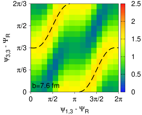
Refer to caption
Figure 16: A fit based on Eq. 39 to the the Glauber data exhibited in Fig. 4. The parameters are B0=0.277(2)subscript𝐵00.2772B_{0}=0.277(2), B2=0.029(1)subscript𝐵20.0291B_{2}=0.029(1), and C=0.532(7)𝐶0.5327C=0.532(7). The normalization (i.e. the color scale) is arbitrary, but is the same as in Fig. 4.

Finally, we can estimate the scaling of these coefficients with the average elliptic eccentricity ϵ2delimited-⟨⟩delimited-⟨⟩subscriptitalic-ϵ2\langle\!\langle\epsilon_{2}\rangle\!\rangle. In a central collision B(ψ1,3,ΨPP)𝐵subscript𝜓13subscriptΨ𝑃𝑃B(\psi_{1,3},\Psi_{PP}) must vanish. This can be understood by examining Fig. 5 and recognizing that in a central collision there is no distinguishable difference between Position A and Position B. The coefficient of cos(3ψ3,3ϕΨPP)3subscript𝜓33superscriptitalic-ϕsubscriptΨ𝑃𝑃\cos(3\psi_{3,3}-\phi^{*}-\Psi_{PP}) (i.e. B𝐵B) describes how phase between the triangular and the dipole planes changes from Position A to Position B. This coefficient must vanish in central collisions where Position A and Position B are identical. Finally the coefficients B2subscript𝐵2B_{2} and C2subscript𝐶2C_{2} reflect the almond shape and must involve an additional power of ϵ2delimited-⟨⟩delimited-⟨⟩subscriptitalic-ϵ2\langle\!\langle\epsilon_{2}\rangle\!\rangle relative to C0subscript𝐶0C_{0} and B0subscript𝐵0B_{0}. With these remarks we arrive at the scalings given in Eq. (42).

References

  • (1)
  • (2) B. Alver and G. Roland, Phys. Rev.  C 81, 054905 (2010) [arXiv:1003.0194 [nucl-th]].
  • (3) J. Adams et al. [STAR Collaboration], Phys. Rev. Lett.  95, 152301 (2005) [arXiv:nucl-ex/0501016].
  • (4) A. Adare et al. [PHENIX Collaboration], Phys. Rev.  C 77, 011901 (2008) [arXiv:0705.3238 [nucl-ex]].
  • (5) B. Alver et al. [PHOBOS Collaboration], Phys. Rev. Lett.  104, 062301 (2010) [arXiv:0903.2811 [nucl-ex]].
  • (6) B. I. Abelev et al. [STAR Collaboration], Phys. Rev.  C 80, 064912 (2009) [arXiv:0909.0191 [nucl-ex]].
  • (7) D. Adamova et al. [CERES Collaboration], Phys. Lett.  B 678, 259 (2009) [arXiv:0904.2973 [nucl-ex]].
  • (8) B. I. Abelev et al. [STAR Collaboration], Phys. Rev. Lett.  102, 052302 (2009) [arXiv:0805.0622 [nucl-ex]].
  • (9) J. Takahashi et al., Phys. Rev. Lett.  103, 242301 (2009) [arXiv:0902.4870 [nucl-th]].
  • (10) P. Sorensen, J. Phys. G 37, 094011 (2010) [arXiv:1002.4878 [nucl-ex]].
  • (11) Z. W. Lin, C. M. Ko, B. A. Li, B. Zhang and S. Pal, Phys. Rev.  C 72, 064901 (2005) [arXiv:nucl-th/0411110].
  • (12) G. L. Ma et al., Phys. Lett.  B 641, 362 (2006) [arXiv:nucl-th/0601012].
  • (13) S. Zhang et al., Phys. Rev.  C 76, 014904 (2007) [arXiv:0706.3820 [nucl-th]].
  • (14) For a review and overview see: D. A. Teaney, arXiv:0905.2433 [nucl-th]. In “Quark-gluon plasma. Vol. 4,” editors R. C. Hwa and X. N. Wang.
  • (15) B. H. Alver, C. Gombeaud, M. Luzum and J. Y. Ollitrault, arXiv:1007.5469 [nucl-th].
  • (16) B. Schenke, S. Jeon and C. Gale, arXiv:1009.3244 [hep-ph].
  • (17) H. Petersen, G. Y. Qin, S. A. Bass and B. Muller, arXiv:1008.0625 [nucl-th].
  • (18) J. Y. Ollitrault, Phys. Rev.  D 46, 229 (1992).
  • (19) P. F. Kolb and U. W. Heinz, arXiv:nucl-th/0305084. In “Quark-gluon plasam. Vol. 3,”, editors, R. C. Hwa and X. N. Wang.
  • (20) B. Alver et al. [PHOBOS Collaboration], Phys. Rev. Lett.  98, 242302 (2007) [arXiv:nucl-ex/0610037].
  • (21) G. Y. Qin, H. Petersen, S. A. Bass and B. Muller, arXiv:1009.1847 [nucl-th].
  • (22) Yan Li and D. Teaney, in progress.
  • (23) B. Alver, M. Baker, C. Loizides and P. Steinberg, arXiv:0805.4411 [nucl-ex].
  • (24) P. Staig and E. Shuryak, arXiv:1008.3139 [nucl-th].
  • (25) P. F. Kolb, J. Sollfrank and U. W. Heinz, Phys. Rev.  C 62, 054909 (2000) [arXiv:hep-ph/0006129].
  • (26) P. Huovinen, P. F. Kolb, U. W. Heinz, P. V. Ruuskanen and S. A. Voloshin, Phys. Lett. B 503, 58 (2001) [arXiv:hep-ph/0101136].
  • (27) N. Borghini and J. Y. Ollitrault, Phys. Lett.  B 642, 227 (2006) [arXiv:nucl-th/0506045].
  • (28) A. P. Mishra, R. K. Mohapatra, P. S. Saumia and A. M. Srivastava, Phys. Rev.  C 77, 064902 (2008) [arXiv:0711.1323 [hep-ph]].
  • (29) A. P. Mishra, R. K. Mohapatra, P. S. Saumia and A. M. Srivastava, Phys. Rev.  C 81, 034903 (2010) [arXiv:0811.0292 [hep-ph]].
  • (30) B. I. Abelev et al. [STAR Collaboration], arXiv:0806.0513 [nucl-ex].
  • (31) B. I. Abelev et al. [STAR Collaboration], Phys. Rev. Lett.  103, 251601 (2009) [arXiv:0909.1739 [nucl-ex]].
  • (32) B. I. Abelev et al. [STAR Collaboration], Phys. Rev.  C 81, 054908 (2010) [arXiv:0909.1717 [nucl-ex]].
  • (33) D. Kharzeev, R. D. Pisarski and M. H. G. Tytgat, Phys. Rev. Lett.  81, 512 (1998) [arXiv:hep-ph/9804221].
  • (34) See the review: S. A. Voloshin, A. M. Poskanzer and R. Snellings, arXiv:0809.2949 [nucl-ex].
  • (35) Sergei Voloshin, private communication.
  • (36) D. Teaney, J. Lauret and E. V. Shuryak, arXiv:nucl-th/0110037. ibid, Phys. Rev. Lett.  86, 4783 (2001)
  • (37) P. F. Kolb, P. Huovinen, U. W. Heinz and H. Heiselberg, Phys. Lett. B 500, 232 (2001) [arXiv:hep-ph/0012137].