IFUM-964-FT
GeF/TH/3-10
Soft gluon resummation
of Drell-Yan rapidity
distributions:
theory and phenomenology
Marco Bonvini,a Stefano Forteb and Giovanni Ridolfia
aDipartimento di Fisica, Università di Genova and
INFN, Sezione di Genova,
Via Dodecaneso 33, I-16146 Genova, Italy
bDipartimento di Fisica, Università di Milano and
INFN, Sezione di Milano,
Via Celoria 16, I-20133 Milano, Italy
Abstract
We examine critically the theoretical underpinnings and phenomenological implications of soft gluon (threshold) resummation of rapidity distributions at a hadron collider, taking Drell-Yan production at the Tevatron and the LHC as a reference test case. First, we show that in perturbative QCD soft gluon resummation is necessary whenever the partonic (rather the hadronic) center-of-mass energy is close enough to threshold, and we provide tools to assess when resummation is relevant for a given process. Then, we compare different prescriptions for handling the divergent nature of the series of resummed perturbative corrections, specifically the minimal and Borel prescriptions. We assess the intrinsic ambiguities of resummed results, both due to the asymptotic nature of their perturbative expansion, and to the treatment of subleading terms. Turning to phenomenology, we introduce a fast and accurate method for the implementation of resummation with the minimal and Borel prescriptions using an expansion on a basis of Chebyshev polynomials. We then present results for and production as well as both high- and low-mass dilepton pairs at the LHC, and show that soft gluon resummation effects are generally comparable in size to NNLO corrections, but sometimes affected by substantial ambiguities.
September 2010
1 Introduction
Drell-Yan rapidity distributions are likely to be the standard candle which is both theoretically calculable and experimentally measurable with highest accuracy at hadron colliders, in particular the LHC. The current QCD theoretical accuracy for this process is NNLO [1], and small effects such as those related to the coupling of the gauge boson to final-state leptons have been studied recently [2]. Whereas the resummation of contributions related to the emission of soft gluons are routinely included in the computation of Drell-Yan transverse-momentum distributions [3], where they are mandatory in order to stabilize the behaviour of the cross-section at low , their impact on rapidity distributions has received so far only a moderate amount of attention. This is partly due to the fact that even in fixed-target Drell-Yan production experiments, such as the Tevatron E866 [4], let alone LHC experiments, the available center-of-mass energy is much larger than the mass of typical final states, thereby suggesting that threshold resummation is not relevant.
However, it has been pointed out since long [5] that because hadronic cross-sections are found convoluting a hard cross-section with a parton luminosity, the effect of resummation may be relevant even relatively far from the hadronic threshold. Indeed, in Ref. [6] threshold resummation has been claimed to affect significantly Drell-Yan production for E866 kinematics, though somewhat different results have been found in Ref. [7]. It is important to observe that Drell-Yan data from E866 and related experiments play a crucial role in the precision determination of parton distributions [8], so their accurate treatment is crucial for precise LHC phenomenology. Furthermore, threshold resummation is known [9] to affect in a non-negligible way standard Higgs production in gluon-gluon fusion at the LHC, even though the process is clearly very far from threshold.
A systematic assessment of the relevance of soft-gluon resummation for rapidity distributions at hadron colliders is called for: it is the purpose of the present paper. We will take the Drell-Yan process as a test case, but our formalism and results can be applied to other collider processes such as heavy quark production or Higgs production.
The main ingredients of this assessment are the following. First, we determine when and why threshold resummation is relevant. Then, we discuss how the resummed contribution is defined, and specifically we deal with the divergence of the series of resummed terms. Next, we address the issue of combining resummed and fixed-order results. Finally, we turn to phenomenology and assess the size and theoretical uncertainty of resummation at the Tevatron and LHC. Each of these steps turns out to be nontrivial, as we now briefly sketch.
The standard physical argument to explain why resummation may be relevant even when the hadronic process is relatively far from threshold goes as follows [10]. The quantity which is resummed in perturbative QCD is the hard partonic cross-section, which depends on the partonic center-of-mass energy and the dimensionless ratio of the latter to the final state invariant mass. Therefore, resummation is relevant when it is the partonic subprocess that is close to threshold. The partonic center-of-mass energy in turn can take any value from threshold up to the hadronic center-of-mass energy, and its mean value is determined by the shape of the PDFs: therefore, one expects threshold resummation to be more important if the average partonic center-of-mass energy is small, i.e. if the relevant PDFs are peaked at small (such as gluons or sea quarks, as opposed to valence quarks). This for instance explains why threshold resummation is especially relevant for Higgs production in gluon-gluon fusion.
We will show that this can be made quantitative using a saddle-point argument in Mellin space: for any given value of the hadronic dimensionless variable the dominant contribution to the cross section comes from a narrow range of the variable which is conjugate to upon Mellin transform. In Mellin space the cross-section is the product of parton distributions (PDFs) and a hard coefficient, but it turns out that the position of the saddle is mostly determined by the PDFs. Moreover, the result is quite insensitive to the non-perturbative (low-scale) shape of the parton distribution and mostly determined by its scale dependence, specifically by the low– (or low–) behaviour of the relevant Altarelli-Parisi splitting functions: the faster the small– growth of the splitting function, the smaller the average partonic center-of-mass energy, the farther from the hadronic threshold the resummation is relevant. This is reassuring, because it means that the region of applicability of threshold resummation is controlled by perturbative physics. The issue of the persistence of sizable soft gluon emission terms even far from threshold was also addressed, using methods of soft-collinear effective theory, in Ref. [7], where in the large region it was related to the (non-perturbative) shape of parton distributions, though it was also observed for smaller values. 111Shortly after this paper appeared in preprint form, the treatment of this issue in soft-collinear effective theory was revisited in a quantitative way in Ref. [11], where it was related to a parameter determined by the shape of parton distributions.
Having established the region in which threshold resummation is relevant, we have to face the fact that resummation sums an infinite series of contributions to the expansion of the hard partonic cross-section in powers of the perturbative strong coupling (with the hard scale of the process) which diverges if the resummation is performed at any given logarithmic order. This divergence can be treated in various ways: here we will consider the minimal prescription (MP) [12] and the Borel prescription (BP) [13, 14], in both of which the resummed result is a function of to which the perturbative expansion in powers of is asymptotic. Both the BP and MP can be obtained by adding to the perturbative series a contribution which removes the divergence, which is power-suppressed in for the BP, and it has support in an unphysical kinematic region (below threshold) for the MP.
In practice, however, different resummation prescriptions differ not only because of the way the high-order divergence of the expansion is handled, but also because if they are applied to a low-order truncation of the divergent series they differ by subleading terms. We will show that in fact this difference turns out to be by far phenomenologically the most significant, unless one is very close to the hadronic threshold, which is in practice a very rare occurrence. We will thus assess the ambiguity that subleading terms induce on resummed results, and to which extent they can be optimized in order to ensure stability of the resummed expansion once resummed results are matched to the standard fixed-order ones.
With one (or more), possibly optimal, resummation prescriptions at hand, we turn to the resummation of rapidity distributions. It turns out that this can be performed by relating the resummed expressions to those of the inclusive cross-section. This entails some further ambiguities in the treatment of subleading terms, though we shall see that these are in practice phenomenologically very small. Finally, we will implement the resummation up to the next-to-next-to-leading log (NNLL) level combined with the next-to-next-to-leading fixed-order (NNLO) result. We will show that this can be done efficiently by projecting resummed results on a basis of Chebyshev polynomials: with this approach, resummed results can be easily obtained using any external set of parton distributions. This will enable us to obtain predictions at the Tevatron and LHC. We will see that even at the LHC the impact of the resummation is not negligible, and comparable to the size of the corresponding fixed-order corrections, especially in the central rapidity region.
The structure of this paper is the following: in Section 2 we will present in detail the arguments which allow one to determine the relevant partonic center-of-mass energy for given hadronic kinematics and parton distribution, and thus to assess the relevance of threshold resummation. In Section 3 we will discuss and compare the minimal and Borel prescription for resummation, the way they can be matched to fixed-order expressions, the way subleading terms are treated with the various prescriptions, and the associate ambiguities. In Section 4 we will present the general formalism for the construction of resummed expressions for rapidity distributions from their inclusive counterparts, and the numerical implementation of resummed results. In Section 5 we will turn to phenomenology for the production of neutral and charged Drell-Yan pairs, with different values of their invariant mass at Tevatron and LHC energies. We will compare theoretical predictions both to E866 and recent CDF data.
2 When is threshold resummation relevant?
As we have mentioned in the introduction, both simple physical arguments and evidence from explicit calculations [10] suggest that threshold resummation may be relevant even quite far from the hadronic threshold, provided the partonic average center-of-mass energy is sizably smaller than the available hadronic center-of-mass energy. Here we derive this conclusion from a quantitative argument, which will allow us to assess the relevance of threshold resummation for a given process. We assess the impact of parton distributions by means of a Mellin-space argument. For a given process and a given value of , we determine the region of the variable , Mellin-conjugate to , which provides the dominant contribution to the cross-section. First, we show that the saddle point is mostly determined by the small– behaviour of the PDFs, which in turn is driven by perturbative evolution. Next, we determine the impact of the inclusion of PDFs for the Drell-Yan process. Finally, with specific reference to the Drell-Yan process, we assess the region where threshold resummation is relevant.
2.1 The impact of PDFs: –space vs. –space
The cross-section for a hadronic process with scale and center-of-mass energy can be written as a sum of contributions of the form
| (2.1) |
in terms of a partonic cross-section and a parton luminosity, in turn determined in terms of parton distributions as
| (2.2) |
Here we denote generically by a suitable quantity (in general, process-dependent) which has the property of factorizing as in Eq. (2.1). Such quantities are usually related in a simple way to cross-sections or distributions; for example, in the case of the invariant mass distribution of Drell-Yan pairs, is in fact .
In general, the cross-section gets a contribution like Eq. (2.1) from all parton channels which contribute to the given process at the given order, but this is inessential for our argument, so we concentrate on one such contribution.
In Eq. (2.1), the partonic cross-section, which is computed in perturbation theory, is evaluated as a function of the partonic center-of-mass energy
| (2.3) |
where and are the momentum fractions of the two partons. Therefore, the threshold region, where resummation is relevant, is the region in which is not much larger than . However, all values of between and are accessible, so whether or not resummation is relevant depends on which region gives the dominant contribution to the convolution integrals Eqs. (2.1, 2.2). This dominant region can be determined using a Mellin-space argument.
The Mellin transform of is
| (2.4) |
with inverse
| (2.5) |
where is larger than the real part of the rightmost singularity of (by slight abuse of notation we denote with both the function and its transform), and in the last step we have defined
| (2.6) |
The function has a singularity on the real positive axis because of the parton luminosity; to the right of this singularity, it is a decreasing function of , because the area below the curve obviously decreases as increases. As a consequence, always has a minimum on the real positive axis at some . Hence, the inversion integral is dominated by the region of around , and can be approximated by saddle-point, expanding around .
When , the slope of the straight line decreases, and the position of the minimum is pushed to larger values, so the large– behaviour of is determined by the large– behaviour of , as it easy to show using the saddle point approximation: in fact, for typical parton distributions in this limit the saddle point approximation becomes exact. This is shown in Appendix A, where some properties of the saddle point approximation to Mellin transforms are collected.
The position of the saddle point is strongly influenced by the rate of decrease of the cross-section as grows. Indeed, in Mellin space, the cross-section Eq. (2.1) factorizes:
| (2.7) |
It is then easy to see that the decrease of with is driven by the parton luminosity : in fact, it turns out that, for large , is an increasing function of . Indeed, it turns out (see Appendix A) that a distribution, unlike an ordinary function, need not be a decreasing function of . However, the parton luminosity always offsets this increase if the convolution integral exists, because the cross-section is an ordinary function. For example, the Drell-Yan partonic cross-section is shown in Fig. 1, where it is clear that even though at small the cross-section decreases with , at large it increases.
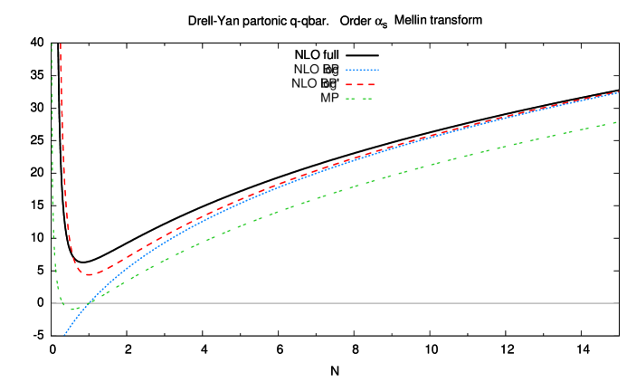
As a consequence, when is large, the position of the saddle point is completely controlled by the drop of the parton luminosity: indeed, in the absence of parton luminosity, the saddle point would be very close to the minimum of the partonic cross-section, which is around . When is smaller, even without PDF the location of the saddle is controlled by the partonic cross-section, which in this region is a decreasing function of . However, this decrease is much stronger in the presence of a luminosity, so the location of the saddle is substantially larger. Hence, in the large region the effect of the resummation is made much stronger by the luminosity, while for medium-small if the luminosity decreases fast enough, may be quite large even if , i.e. far from the hadronic threshold, thereby extending the region in which resummation is relevant.
The position of the saddle point in the various regions can be simply estimated on the basis of general considerations. At the leading log level, parton densities can be written as linear combinations of terms of the form
| (2.8) |
where are eigenvalues of the leading-order anomalous dimension matrix:
| (2.9) |
and are initial conditions given at some reference scale . The cross-section is correspondingly decomposed into a sum of contributions, each of which has the form of Eq. (2.5), with
| (2.10) |
At large , this expression is dominated by the first term, which grows linearly with , while at small the behaviour of is determined by the singularities of the anomalous dimensions, which are stronger than those of the initial conditions if , given that low-scale physics is both expected theoretically from Regge theory [15, 16] and known phenomenologically from PDF fits [17] to produce at most poles but not essential singularities such as those obtained exponentiating the anomalous dimensions. Indeed, assuming a power behaviour for both at small and large ,
| (2.11) |
so that
| (2.12) |
behaves as both at large and small , and is thus subdominant in comparison to either the dependent term or the anomalous dimension contribution in Eq. (2.10). A similar argument holds for the partonic cross-section term .
The position of the minimum is therefore determined by the transition from the leading small– drop due to the anomalous dimension term and the leading large– rise due to the –dependent term, up to a correction due to the other contributions to Eq. (2.10). When is large, the rise in the first term is slow, and it only sets in for rather large so the correction due to the other contributions may be substantial. This is the region in which resummation is surely relevant because the hadronic is large. But when is not so large, the rise sets in more rapidly, in the region where the second term is dominant and the correction from the initial PDFs and the partonic cross-section is negligible.
In order to provide an estimate of the value of in either region, we note that the leading-order Altarelli-Parisi anomalous dimensions at small behave as
| (2.13) |
where “less singular” denotes terms whose singularity has a smaller real part, and for , and for . This implies that one of the two singlet anomalous dimension eigenvectors has a leading singularity at , while the other has a singularity at and it is thus suppressed at small , like the nonsinglet anomalous dimension which is thus also suppressed. This pattern persists to all perturbative orders. It follows that singlet quark and gluon distributions have a steeper small– and thus small– behaviour.
Expanding the anomalous dimension about its rightmost singularity at leading order we have
| (2.14) |
where and are respectively the dominant small– singlet eigenvalue and nonsinglet anomalous dimension, and
| (2.15) |
We note that (because of momentum conservation), while (because of baryon number conservation): hence, we expect the small approximation Eqs. (2.14, 2.15) to break down around , with
| (2.16) |
We can then consider three cases, according to whether , in Eq. (2.10) are both singlet, both nonsinglet, or one singlet and one nonsinglet. The three cases correspond respectively to the leading behaviour of, for instance, Higgs production in gluon fusion, Drell-Yan production at the Tevatron, and Drell-Yan production at the LHC. Substituting Eq. (2.14) in Eq. (2.10) and neglecting the last three terms the saddle is found to be at
| (2.17) |
where take the values and , are given by Eq. (2.16), and
| (2.18) |
We expect Eq. (2.17) to provide a good approximation to the position of the saddle point in the region , while for larger values of the last three terms on the right-hand side of Eq. (2.10) provide a correction of increasing size. This correction cannot be estimated in a universal way, in that it will generally depend on the shape of the initial parton distributions . However, note that at large both the nonsinglet and singlet anomalous dimension drop: they are negative, and their modulus grows as . Furthermore, , which, together with Eqs. (2.11, 2.12) implies that also the contributions from to Eq. (2.10) drop logarithmically as . This drop is a generic feature of the initial PDFs: it is necessary in order for the convolution integral which gives the physical cross-section to exist (see Appendix A); likewise, the drop of the anomalous dimension (at most as a power of ) is a generic feature of perturbative evolution, related to momentum conservation of gluon radiation, and it persists to all orders.
It follows that at large the drop Eq. (2.14) is replaced by a slower logarithmic drop, with a coefficient determined by both the large– behaviour of the anomalous dimension and by the initial PDFs. This leads to a rather larger value of the saddle point than given by Eq. (2.17).
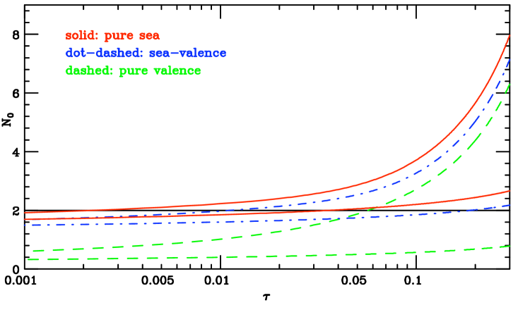
The value of as a function of given by Eq. (2.17) is plotted in Fig. 2 for the three cases of Eq. (2.18): in each case, we show both the result obtained using the approximation Eq. (2.17), and that found by exact numerical minimization of Eq. (2.10), with the full leading-order expression of the pertinent anomalous dimensions , , and initial PDFs of the form Eq.(2.11), with
| (2.19) |
but still neglecting the . We see that indeed the pole approximation Eq. (2.17) holds reasonably well for .
We can get a feeling for the implication of this for the region in which resummation is relevant by very roughly taking the value as that of the transition from the small– region to the large– region. Indeed, this value corresponds to the energy-momentum operator and it thus sets the transition between the large region in which parton distributions drop (while growing in modulus) and the small region in which they grow as the scale is raised. This rough estimate is borne out by a more quantitative assessment of the transition point which will be performed in Sect. 2.3. We then see that, if at least one of the parton distributions is flavour singlet, the position of the saddle point remains in the large– region down to fairly low values of . This extension of the region where resummation is relevant to small is due to the rise of the anomalous dimension related to the pole at Eq. (2.13) in the singlet sector.
Larger values of correspond to values of which are anyway in the large– region. However, in this region the rapid drop of the parton distribution, due both to its initial shape and to its evolution, greatly increases the impact of resummation by raising the position of the saddle, which at is already .
2.2 The impact of PDFs: the Drell-Yan process
We now assess the impact of parton distributions in the specific case of Drell-Yan production. In this case, the quantity which appears in Eq. (2.1) is given by
| (2.20) |
where is the invariant mass distribution of Drell-Yan pairs. The corresponding partonic quantity of Eq. (2.1) is then
| (2.21) |
It is further convenient to define a dimensionless coefficient function through
| (2.22) |
The coefficient function admits the perturbative expansion
| (2.23) |
the Born term contains the electroweak coupling and it is given e.g. in Ref. [18]. Threshold logarithms only appear in the quark–antiquark channel, while in other partonic channels they are suppressed by powers of . In the quark–antiquark channel the next-to-leading order contribution is given by [19]
| (2.24) |
Note that of course at leading order is just a constant. The Mellin transform of the NLO term is
| (2.25) |
and was shown in Fig. 1.
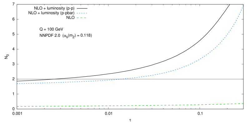
We have then determined the position of the saddle point in a realistic situation, i.e., using the partonic cross-section Eq. (2.25) for Drell-Yan production of a neutral lepton pair of invariant mass GeV at a or collider, with a parton luminosity determined using NNPDF2.0 [8] parton distributions. Comparing the realistic curves of Fig. 3 to those in Fig. 2, which were determined using the toy initial PDFs Eqs. (2.11, 2.19) and neglecting the contribution from the hard cross-section we see that the curve of Fig. 3 agrees well with the sea–valence curve of Fig. 2, as one would expect given that in collisions one must always pick up at least a sea (antiquark) PDF. The case of is slightly more subtle: in this case, for the curve in Fig. 3 agrees well with the valence–valence curve of Fig. 2. However, for smaller values of the position of computed using the full luminosity decreases much more slowly: this is due to the fact that as the contribution rapidly grows due to the pole Eq. (2.14) so that even the valence distribution is dominated by it. As a consequence, even in the the resummation region is further extended to somewhat lower values than it would be the case for a pure valence–valence luminosity.
In Fig. 3 we also show the position of the saddle that is obtained if the parton luminosity is omitted, i.e. for the parton-level cross-section. It is clear that, as we argued in Sect. 2.2, the position of the saddle is determined by the PDFs, and it is much larger than that found at the parton level, thereby supporting the conclusion that the convolution with the parton luminosity greatly enhances the importance of resummation, and it extends it to a much wider kinematic region.
In summary, we conclude that the resummation region corresponds to for collisions, and for collisions. For the position of the saddle is determined by the pole in the anomalous dimension, while for larger values of the large drop of PDFs, due both to their initial shape and to perturbative evolution, very substantially enhances the impact of resummation. These values have been obtained for GeV. We have checked that they depend very weakly on , which is expected, because enters the determination of the saddle point only through the scale dependence of the parton densities.
2.3 The resummation region for the Drell-Yan process
Having established that the PDFs drive the position of the saddle point, and having explicitly determined this value, we now have to determine quantitatively the value of at which resummation becomes important. So far, we have taken conventionally the momentum-conservation point as the value at which logarithmically enhanced contributions give a sizable contribution to the cross-section. We would now like to establish this in a quantitative way.
To this purpose, we compare Eq. (2.25) to its logarithmic approximation. The logarithmically-enhanced term in Eq. (2.25) is
| (2.26) |
whose Mellin transform is
| (2.27) |
The function was displayed as a function of along the real positive axis in Fig. 1. The logarithmic approximation Eq. (2.27) is also shown in the same figure. It is clear that the full result and the log approximation agree at large , up to a small constant shift. Indeed,
| (2.28) |
For slightly above 2 the logarithmic contribution is already about 50% of the full result, but it rapidly deviates from it as decreases. This suggests that indeed the logarithmic contribution is sizable for .
It is interesting to observe that there is a certain arbitrariness in the definition of the logarithmically enhanced contribution: indeed, the Mellin transform Eq. (2.27) of the logarithmic contribution Eq. (2.26) contains terms which are not logarithmically enhanced in –space: the Mellin transform of the nextk-leading-log expression only coincides with the nextk-leading-log expression up to subleading terms. For example, , so that we could equally well identify the logarithmically enhanced contribution to Eq. (2.25) with
| (2.29) |
which is the Mellin transform of
| (2.30) |
In other words, logarithmically enhanced contributions in –space also contain subleading terms when transformed to –space, and conversely (see Appendix B for details on the relevant Mellin transforms).
The curve corresponding to is also shown in Fig. 1. It is clear that in the large region it differs from by a negligible amount. However, at small this particular logarithmic approximation turns out to be much closer to the full result. Whereas of course the choice of subleading terms to be included in the resummation is essentially arbitrary, in practice some choices may be less natural than others: this will be discussed in Sect. 3.2 below.
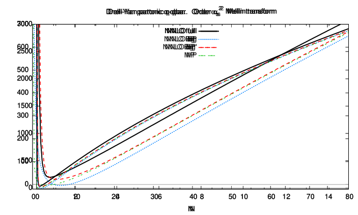
In order to check that these conclusions are generic, we repeat the comparison at the next perturbative order. The order Drell-Yan cross-section has been computed in Ref. [20]. In Fig. 4 it is compared to its logarithmic approximation , defined as the Mellin transform of all contributions to which grow logarithmically as , as well as another logarithmic approximation which differs by the former through power-suppressed terms, analogous to and to be discussed in more detail in Sect. 3.2 below.
It is apparent from Fig. 4 that the conclusions drawn at NLO are qualitatively unchanged, though there is some quantitative difference: the logarithmic approximation, which differs by a constant from the asymptotic large– behaviour of the coefficient function, provides a sizable or even dominant contribution to it for , according to the choice of subleading terms: approximations which differ by subleading terms are all very close for , though they may differ substantially at small .
As a final comment we note that the region in which we have found logarithmic effects to be important is in fact rather wider than the region in which . In this region even though logarithmically enhanced terms may lead to a substantial contribution, they behave in an essentially perturbative way, in that , and therefore the all-order behaviour of the resummation is irrelevant. In this intermediate region, the resummation may have a significant impact, but with significant ambiguities related to subleading terms.
3 Resummation
After having provided an assessment of the kinematic region in which logarithmically enhanced terms are significant, we now discuss their all-order resummation. We will assume knowledge of the resummed results in –Mellin space, both at the level of inclusive cross-sections [21, 22, 23] and rapidity distributions [24, 25, 6], and we will concentrate on the ambiguities related to their definition. First, we briefly review some prescriptions introduced in order to deal with the divergent nature of the perturbative expansion for resummed quantities. Next, we discuss the role and impact of subleading terms in the resummation, with specific reference to the subleading terms which are introduced by different resummation prescriptions.
3.1 Resummation prescriptions
Resummation of the partonic cross-section Eq. (2.1) is most naturally performed in space, because the solution of the relevant Altarelli-Parisi equation [22], the relevant factorization theorem [21, 26] and the relevant renormalization group equation [26, 23] are all naturally formulated in –space. The underlying physical reason is that, in the soft limit, while amplitudes factorize due to the eikonal approximation both in – and in –space, the relevant phase space only factorizes in –space but not in –space [27].
Recently, resummation has also been performed using SCET techniques both in –space [28] and in momentum space [29, 7]; in the latter approach the soft scale whose logarithms are resummed is not the partonic scale but rather a soft scale , independent of the parton momentum fraction , but related to the hadronic scale . As a consequence, the hard coefficient function depends on not only through the convolution variable, but also directly through the soft scales: therefore, the resummed result can no longer be factorized by Mellin transformation into the product of a parton density and a hard coefficient. For this reason, a direct comparison between the result obtained through the SCET approach and that based on standard factorization Eq. (2.1) is not possible at the parton level. A phenomenological comparison is possible [7], but it requires either assuming a specific form of the parton distribution functions, or switching to a SCET formulation in which depends on , which however is not the Mellin transform of the –space SCET result, advocated for phenomenolgy in Ref. [7].
The general structure of –space resummed expressions can be understood by considering the case of the inclusive coefficient function , obtained by Mellin transformation from Eq. (2.23). At the resummed level,
| (3.1) | ||||
| (3.2) | ||||
| (3.3) |
where is a process-dependent constant ( for Drell-Yan production). At the nextk-to-leading logarithmic (NkLL) level functions up to must be included, and must be computed up to order (see Appendix D for explicit expressions). Expansion of the resummed coefficient function Eq. (3.1) in powers of up to order gives the logarithmically enhanced contributions to the fixed-order coefficient functions Eq. (2.23) up to the same order, with, at the NkLL level, all terms of order with correctly predicted. The inclusion up to the relevant order of the function is necessary, despite the fact that does not depend on , because of its interference with the expansion of the exponentiated logarithmically enhanced functions with .
Matched resummed coefficient functions are then obtained by combining the resummed result Eq. (3.1) with the fixed-order expansion in power of , and subtracting double-counting terms, i.e. the expansion of in powers of up to the same order:
| (3.4) |
However the perturbative expansion of Eq. (3.1) in powers of turns out to be divergent. This follows from the fact that the functions in Eq. (3.2) depend on through
| (3.5) |
with defined in Eq. (3.3). As a consequence, the expansion of the resummed partonic cross-section in powers of has a finite radius of convergence dictated by , and at fixed has a branch cut in the complex –plane along the positive real axis from to . But a Mellin transform always has a convergence abscissa, so cannot be a Mellin transform.
On the other hand, any finite-order truncation of the series expansion
| (3.6) |
behaves as a power of at large and it is thus free of singularities for large enough. Hence, can be viewed as the Mellin transform of the function
| (3.7) |
such that
| (3.8) |
It follows, by contradiction, that the series Eq. (3.7) must diverge [13]. It turns out [13] that, if the Mellin inversion Eq. (3.8) is performed to finite logarithmic accuracy, the series Eq. (3.7) acquires a finite but nonzero radius of convergence in ; however, this does not help given that the convolution integral Eq. (2.1) always goes over the region where the series diverges.
Hence, any resummed definition must either explicitly or implicitly deal with the divergence of the perturbative expansion Eq. (3.7). We now consider two prescriptions in which this is done by constructing a resummed expression to which the divergent series is asymptotic.
3.1.1 Minimal prescription
The minimal prescription (MP) [12] defines the resummed hadronic cross-section as
| (3.9) |
where is defined in Eq. (2.22). The integration path in Eq. (3.9) is taken to the left of the cut, but to the right of all other singularities. It is shown in Ref. [12] that the cross-section obtained in this way is finite, and that it is an asymptotic sum of the divergent series obtained by substituting the expansion Eq. (3.6) in Eq. (3.9) and performing the Mellin inversion order by order in . Of course, if the expansion is truncated to any finite order the MP simply gives the exact inverse Mellin transform, namely, the truncation of Eq. (3.7) to the same finite order.

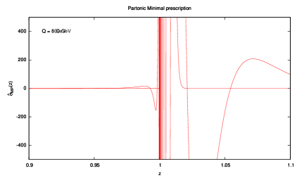
If the MP is applied to the resummed partonic cross-section, i.e. if one omits the parton luminosity in Eq. (3.9) then, because of the branch cut to the right of the integration contour, the ensuing integral gives a function , which does not vanish when [12]. However, as shown in Ref. [12], the contribution from the region is exponentially suppressed in . In the vicinity of the integral oscillates strongly, as shown in Fig. 5, where is displayed for the Drell-Yan resummed cross-section, evaluated at two scales which are relevant for the phenomenological discussion of Sect. 5. When folded with the luminosity, the hadronic cross-section receives a contribution from the unphysical region and the corresponding integral thus does not have the form of a convolution. The ensuing integral is finite, but the oscillatory behaviour of the partonic cross-section makes its numerical computation difficult. A technical solution to this problem is provided in Ref. [12]; here, we will propose in Sect. 4 a different solution, and use it for phenomenology in Sect. 5.
3.1.2 Borel prescription
An alternative prescription is based on the Borel summation of the divergent series. This prescription was developed in Refs. [13, 14]; here we give an equivalent, but a somewhat simpler presentation of it. To this purpose, it is convenient to rewrite the resummed coefficient function Eq. (3.1) as
| (3.10) |
where is the (–independent) Born result, so that only logarithmically enhanced terms are included in . Using Eq. (B.6) we see that
| (3.11) |
where
| (3.12) |
and are the coefficients of the expansion
| (3.13) |
whose dependence will henceforth be omitted for notational simplicity. Using Eq. (B.5) Eq. (3.11) can be written as
| (3.14) |
The Borel prescription can be now formulated. First, we note that the Borel transform of with respect to , which is found replacing
| (3.15) |
in Eq. (3.14), is convergent, and can be summed in closed form:
| (3.16) |
The branch cut of , , is mapped onto the range on the real axis of the complex plane. Hence, the integration path is any closed curve which encircles the cut.
Next, we observe that the inverse Borel transform of does not exist because it involves evaluation of the function on the negative real axis where it is badly behaved as [13]. We may however define the inversion integral by introducing a cutoff at some finite value of the Borel variable : if we replace Eq. (3.14) with
| (3.17) |
then the resummed function becomes
| (3.18) |
It is proved in Refs. [13, 14] that the original divergent series Eq. (3.11) for is asymptotic to the function , and furthermore, that for any finite-order truncation of the divergent series, the full and cutoff results differ by a twist– term, where is the cutoff. The parameter can be chosen freely in the range (with as in Eq. (3.3)), with different choices differing by power suppressed terms. We will use henceforth the “minimal” choice .
A somewhat simpler result is obtained if the Borel transform is performed through the replacement
| (3.19) |
in Eq. (3.14), instead of Eq. (3.15). In this case, instead of Eqs. (3.17, 3.18) one gets
| (3.20) | ||||
| (3.21) |
which differs from Eq. (3.17) by higher-twist terms, and therefore provides an equally good resummation prescription; the difference is in practice very small.
If we only wish to retain terms which do not vanish as we may expand
| (3.22) |
with the result
| (3.23) |
Equations (3.18), (3.21), and (3.23) provide three alternate definitions of the resummed function which differ by terms suppressed by powers of . The difference between the first two is negligible and the prescription Eq. (3.18) will not be discussed further, but Eqs. (3.21) and (3.23) differ by a sizable amount, as we shall see in somewhat greater detail in Sect. 3.2. Equation (3.23) with is the default Borel prescription of Ref. [13, 14].

When using the Borel prescription, the divergent series Eq. (3.7) is made convergent by cutting off its high-order behaviour: indeed, using the Borel prescription Eq. (3.21) to compute the inverse Mellin transform of one gets
| (3.24) |
and similarly if the Borel prescription Eq. (3.23) is adopted instead. Equation 3.24 differs from the exact result Eq. (B.4) by the factor [13], given by
| (3.25) |
where is the truncated Gamma function. This factor, plotted in Fig. 6, effectively truncates the series before the divergence sets in.
3.2 Subleading terms
The Borel and minimal prescriptions summarized in Sect. 3.1 differ in the way the high-order behaviour of the divergent series is handled. This, as discussed in Refs. [13, 14], makes in practice a small difference unless the hadronic is close to the Landau pole of the strong coupling, , which is seldom the case, and never for applications at collider energies that we are mostly interested in. This is a consequence of the fact that for values of in the perturbative region it is only at very high orders that the effect of the various prescriptions kicks in. For example, with the Borel prescription and the “minimal” choice , if then , so from Fig. 6 one sees that the perturbative expansion is truncated between the tenth and twentieth order.
However, prescriptions may also differ in the subleading terms which are introduced when performing the resummation. To understand this, consider the result one gets applying the various prescriptions to any finite truncation of the expansion of in powers of . The minimal prescription then just gives the exact Mellin inverse Eq. (B.6). Because this result depends on through , in space it generates a series of power suppressed terms Eq. (3.22).
If the Borel prescription is defined according to Eq. (3.21), then the result Eq. (3.24) is obtained, which for small enough that coincides with the minimal prescription, including subleading terms. However, with the Borel prescription the dependence is under analytic control: it is entirely contained in the factor in Eq. (3.21), and it can thus be modified at will. Indeed, while the original Borel prescription Eq. (3.21) treats subleading terms as the minimal prescription, and thus it coincides with it for finite not too high order truncations of the perturbative expansion, using our default Borel prescription Eq. (3.23) instead of Eq. (3.21) only leading power contributions in are retained. However, this implies that power-suppressed contributions in are introduced: indeed, the exact Mellin transforms of Eq. (3.21) and Eq. (3.23) are respectively given by
| (3.26) |
which differ by terms suppressed by powers of .
Hence, the BP Eq. (3.23) on the one hand, and the MP (and the BP Eq. (3.18)) on the other hand correspond to two opposite extreme choices in the treatment of subleading terms: in the MP, all powers suppressed terms in –space are set to zero, but this leads to power suppressed terms in space, while in the BP the opposite is true. The difference between the MP and the default BP Eq. (3.23) could thus be taken as a maximal estimate of the impact of subleading terms.
With the Borel prescription it is also possible to construct intermediate, possibly optimized, choices of subleading terms. Indeed, in Sect. 2.3 we have noticed that in the case of the NLO coefficient function , the Mellin transform Eq. (2.27) of the logarithmically enhanced –space terms can be brought in better agreement with the full result by inclusion in it of some terms suppressed by powers of — see , defined in Eq. (2.29). This increased agreement can be understood by inspection of the –space expression of the improved result, Eq. (2.30): the extra power-suppressed terms which are introduced in it turn out to be present in the full result. These terms are in fact of kinematical origin: soft resummation follows from the kinematic fact that as the dependence of partonic cross-sections on is always in the combination [23], essentially because this is the upper limit of the integral over the energy of radiated gluons for the Drell-Yan process. However, the upper integration limit is really
| (3.27) |
so that in fact the resummation produces logarithmic terms of the form .
This suggests to define an all-order generalization of the approximation , by simply letting
| (3.28) |
in all resummed expressions. In the Borel prescription, this is easily done:
| (3.29) |
With this choice, the kinematic correction Eq. (3.28) is automatically included to all orders. However, beyond other subleading terms of the same form but not of kinematic origin will in general be present. This choice also arises in a natural way in the context of soft-collinear effective theories, and it was adopted in Ref. [7].
It turns out that the modified Borel prescription (BP′) Eq. (3.29) is closer to the MP than the default one Eq. (3.23) because
| (3.30) |
so that
| (3.31) |
Equation (3.31) shows that, amusingly, up to terms suppressed by two powers of , the minimal prescription effectively also performs the kinematic subleading replacement Eq. (3.28), though at the cost of also introducing an overall factor which is absent in the known perturbative contributions.

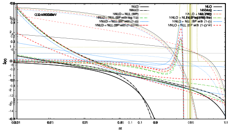


In order to assess the impact of these different prescriptions, in Fig. 7 we compare the matched result Eq. (3.4) for the Drell-Yan coefficient function in the quark–antiquark channel obtained by including terms up to NLL in the resummed expression, and either up to (NLO) or (NNLO) in the fixed-order expansion, with various resummation prescriptions. First, we note that the minimal prescription and the Borel prescription Eq. (3.21) (denoted as BP with in the figure) are essentially indistinguishable (for values of less than about 0.9, where the oscillatory behaviour of the minimal prescription sets in). This is what one expects, since they contain the same subleading terms and they only differ in the treatment of the high-order divergence.
However, the Borel prescription Eq. (3.23) is seen to differ by a non-negligible amount from the minimal prescription: at large where the resummation kicks in it is small in comparison to the size of the resummation itself, while at small , where the resummation just leads to unreliable subleading contributions, it is smaller than the typical higher order correction, as it is seen by comparing results matched to the NLO and NNLO. However, in the intermediate region the subleading terms introduced by this prescription are uncomfortably large.
The improved BP′ Borel prescription Eq. (3.29) (denoted as BP with in the figure) as expected differs less from the MP both at large and at small ; also, it does not introduce unnaturally large subleading terms for any value of . The difference between MP and this last version of the Borel prescription is not negligible but small in comparison to the size of resummation effects in the region where the resummation is relevant, and it is smaller than typical higher-order terms in the region in which the resummation is not relevant. It can thus be taken as a reliable estimate of the ambiguity in the resummation. It is interesting to observe that the subleading terms which are introduced by the replacement Eq. (3.28) grow at small , and in fact are thus reproducing part of the small– growth of perturbative coefficient functions. The fact that inclusion of these terms is important in keeping the ambiguities of large resummation under control suggests that the large and small resummation regions are not well separated, and that there might be an interplay between small– and large– resummation.
4 Rapidity distribution
The resummed expression for rapidity distributions was only derived relatively recently in Refs. [25, 6], confirming a conjecture of Ref. [24]. In this Section, after introducing rapidity distributions at fixed perturbative order, we will briefly review this result, and also compare it to a somewhat different expression later derived using SCET methods in Ref. [7]. We will then discuss the numerical implementation of resummed results that will be used for phenomenology in Sect. 5.
The hadronic rapidity distribution for a Drell-Yan pair of invariant mass produced in hadronic collisions at center-of-mass energy is given by
| (4.1) |
where
| (4.2) |
The sum runs over all partons in hadrons and . To simplify notations, in the following we suppress the explicit dependence of the partonic cross-sections on and on the factorization and renormalization scales . We define
| (4.3) |
so that
| (4.4) |
Especially in fixed-target experiments, distributions sometimes are given in terms of the Feynman variable instead of rapidity. The variable is defined by
| (4.5) |
where is the longitudinal momentum of the Drell-Yan pair, and it is related to the rapidity and the transverse momentum by
| (4.6) |
where . At leading order , and at NLO is fixed uniquely in terms of by the kinematics, so up to this order the and rapidity distributions are simply proportional:
| (4.7) |
though at higher orders they will be different.
4.1 Fixed-order results
At next-to-leading order, the rapidity distribution receives contributions from quark–antiquark and quark–gluon subprocesses:
| (4.8) |
The result is conveniently expressed in terms of new variables , defined by
| (4.9) |
with inverse
| (4.10) |
The partonic threshold region corresponds to .
At order the contribution is given by
| (4.11) |
where we have defined
| (4.12) |
the constants are suitable combinations of the coupling constants of partons to vector boson, and
| (4.13) |
The contribution is given by
| (4.14) |
where
| (4.15) |
and
| (4.16) |
The inclusive coefficient functions, whose form in the quark–antiquark channel and for has already been discussed in Sect. 2.2, are found integrating over the hadronic rapidity . We get
| (4.17) |
with
| (4.18) | ||||
| (4.19) |
and
| (4.20) | |||||
| (4.21) |
where was given in Eq. (2.24) and
| (4.22) |
The NNLO rapidity distribution has been computed in Ref. [1], where its lengthy analytic expression can be found.
4.2 Resummation
As already mentioned, large threshold logs only appear in the quark–quark channel, while the contributions from other channels are suppressed by at least one more power of as in comparison to the contribution. We therefore consider the term of Eq. (4.4),
| (4.23) |
where is the quark-antiquark coefficient function, which is independent of the flavour of the colliding quarks.
Threshold resummation of rapidity distributions is based on the observation [25, 6] (conjectured in Ref. [24]) that at large the coefficient function factorizes as
| (4.24) |
where is the rapidity-integrated coefficient. This is easily proved by rewriting in terms of its Fourier transform with respect to :
| (4.25) |
The integration range in Eq. (4.25) is restricted by kinematics to . Hence, one may expand the exponential in powers of ,
| (4.26) |
where is the rapidity-integrated coefficient function. Hence, is independent of up to terms which as are suppressed by powers of , and one immediately gets the desired factorized form:
| (4.27) |
Up to power-suppressed terms we can thus write
| (4.28) |
Because Eq. (4.28) only depends on the rapidity-integrated coefficient function, threshold resummation is simply performed by using for the latter the resummed expressions discussed in Sect. 3.
Note that resummation of the distributions can be performed in the same way. This is because the kinematical bounds on ,
| (4.29) |
translates into
| (4.30) |
and a similar relation holds at the partonic level. Hence the the above argument holds for the distribution as well.
The dependence on parton distributions in Eq. (4.28) can be easily rewritten in terms of the differential parton luminosity Eq. (4.12) with fixed values of the momentum fractions . To this purpose, perform the change of variables
| (4.31) |
with the inverse
| (4.32) |
The line , selected by the delta function, is contained in the integration region for all values of in
| (4.33) |
Hence,
| (4.34) |
where we have used Eq. (4.12). The integration range in Eq. (4.34) can be extended down to because vanishes for :
| (4.35) |
By inspection of Eq. (4.9), we see that, for , depend on through the ratio . Therefore, Eq. (4.35) has the form of a convolution product: this greatly simplify its treatment, which is then analogous to that of the resummed integrated cross-section, with the replacement
| (4.36) |
The matched resummed expression for the Drell-Yan cross-section can finally be written in analogy to Eq. (3.4):
| (4.37) |
Before turning to the numerical implementation of the resummed result, we discuss briefly a different way of relating the resummation of rapidity distribution to that of the inclusive cross-section which has been more recently presented in Ref. [7]. This is based on writing the rapidity distribution in terms of the variables defined in Eqs. (4.9, 4.10):
| (4.38) |
with
| (4.39) |
It is then observed that at NLO the logarithmically enhanced terms in the partonic threshold limit appear as coefficients of the combination , as one can check by inspection of Eq. (4.13). At higher orders, logarithmic terms in general multiply non-trivial functions of , but Eq. (4.9) implies that the dependence of is of order , so
| (4.40) |
Hence
| (4.41) |
where
| (4.42) |
as it is easily seen integrating Eq. (4.40) with respect to between 0 and 1 and noting that
| (4.43) |
It follows that
| (4.44) |
Equation (4.44) differs by power suppressed terms from the resummed result previously derived Eq. (4.35), as it is easy to check explicitly. Indeed, using Eq. (4.9) and expanding , and in powers of about it is easy to check that
| (4.45) |
Because the difference is suppressed by two powers of one expects it to be small, and indeed we have checked that (using the Borel prescription) the difference between Eqs. (4.35) and (4.44) is negligible, and specifically much smaller than the difference between Borel and minimal prescription.
We note that, because and are not functions of , the form Eq. (4.44) of the resummed result does not have the structure of a convolution and thus would require a separate numerical implementation. For the same reason, a comparison between Eqs. (4.35) and (4.44) using the minimal prescription cannot be performed, because Eq. (4.44) cannot be expressed in terms of the Mellin transform of . We will disregard the form Eq. (4.44) of rapidity distributions henceforth.
4.3 Numerical implementation
For the sake of phenomenology, an efficient numerical implementation of resummed results using the various prescriptions is necessary. Such an implementation was hitherto not available and it will be discussed here.
The minimal prescription involves the numerical evaluation of the complex integral
| (4.46) |
where the integration path is usually chosen as in Fig. 8 in order to make the integral absolutely convergent.

However, parton densities obtained from data analysis are commonly available as functions of in interpolated form through common interfaces such as LHAPDF [30], and the numerical evaluation of their Mellin transform does not converge along the path of integration (specifically, for ) and must be defined by analytic continuation. The option of applying the MP to the partonic cross-section, and then convoluting the result with the parton luminosity in momentum space is not viable, because the MP does not have the structure of a convolution: the partonic cross-section does not vanish for , and it oscillates wildly in the region . This problem is discussed in Ref. [12], where it is handled by adding and subtracting the results of the minimal prescription evaluated with a fake luminosity which allows for analytic integration.
Another possibility, adopted for example in Ref. [6], is to use parton distributions whose Mellin transform can be computed exactly at the initial scale. This, however, greatly restricts the choice of parton distributions, and specifically it prevents the use of current state-of-the-art PDFs from global fits. It is thus not suitable for precision phenomenology.
The method adopted here, based on an idea suggested long ago [31], consists of expanding the function (or for the inclusive cross-section) on a basis of polynomials whose Mellin transform can be computed analytically. We have chosen Chebyshev polynomials, for which efficient algorithms for the computation of the expansion coefficients are available. The details of the procedure are illustrated in Appendix C. The obvious drawback of this procedure is that it must be carried on for each value of the scale and, in the case of rapidity distribution, for each value of and .
We now turn to the discussion of an implementation issue which is specific to the Borel prescription (BP), and has to do with the choice of the cutoff . As discussed in Sect. 3.1.2 the minimal choice is ; however when the integration path in Eq. (3.23) includes values of with , for which the convolution integral diverges. As discussed in Ref. [14], the integral can be nevertheless defined by analytic continuation, by subtracting and adding back from its Taylor expansion in around : the subtracted integrals converge, and the compensating terms can be determined analytically and continued in the desired region.
Here we propose a different method which is numerically much more efficient. The idea is to perform the convolution integral with the luminosity analytically, before the complex integral of Eq. (3.29). When we can use the identity
| (4.47) |
under the integral, because the two ensuing integrals are separately convergent. We get
| (4.48) |
where we have defined
| (4.49) |
The function is more easily approximated by an expansion on the basis of Chebyshev polynomials than . Proceeding as in Appendix C.2 we find
| (4.50) |
where is the order of the approximation, and the coefficients can be computed by numerical methods. We have
| (4.51) |
where
| (4.52) |
is the incomplete Beta function. The function is singular at . In Eq. (4.51), the first argument of the B functions in the integrand vanishes for non positive integer values of , in correspondence of zeros of . Thus, the integrand has only a branch cut in . This expression is in fact valid for arbitrarily large values of , hence it can also be used in the case , which requires multiple subtractions if the method of Ref. [14] is used.
The rapidity distribution is obtained by repeating the above procedure with
| (4.53) |
Since vanishes for , the convolution integral is actually restricted to the region . This difference amounts to replacing by :
| (4.54) |
5 Phenomenology
We will now turn to a phenomenological assessment of the impact of resummation for Drell-Yan invariant mass and rapidity distributions. As discussed in Sect. 1, threshold resummation is not currently included in the calculations of fixed-target and collider Tevatron Drell-Yan data which are included in global parton fits such as MSTW08 [32], NNPDF2.0 [8], or CT10 [33]; neither it has been so far included in predictions for the LHC, such as those of Ref. [34].
We will therefore consider three cases: collisions at a center-of-mass energy of 38.76 GeV, which corresponds to the case of the experiment E866/NuSea, taken as representative of Tevatron fixed-target experiments; collisions at the Tevatron collider energy of TeV; and the LHC case, collisions at the intermediate energy of TeV and at the design energy TeV. For the Tevatron and LHC configurations, we will consider both charged () and neutral () Drell-Yan pairs, taking into account in the latter case the interference between virtual and . Lepton masses will always be neglected. We will show results for both the invariant mass distribution as a function of , and for the doubly-differential distribution in invariant mass and rapidity as a function of the rapidity for fixed values of . Specifically, for invariant mass distributions we will show results for the -factor defined as
| (5.1) |
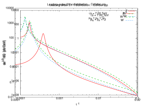
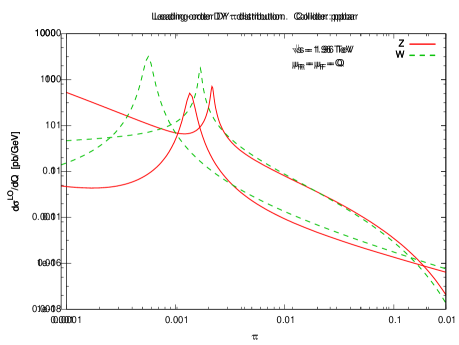
where and are the factorization and renormalization scale, respectively. Since we will be considering different experimental configurations, the results for the -factors will be shown for fixed value of , with determined by the value of , . The Born cross-section , which provides the scale for these plots, is shown in Fig. 9 for LHC at TeV and Tevatron at TeV.
Our aim will be to assess the potential impact of inclusion of resummation effects on cross-sections and their associate perturbative uncertainty, both on experiments which are already used for PDF determinations (and thus, potentially, on the PDF extraction itself), as well as on future LHC measurements, both for real and production as well as for high-mass 1 TeV Drell-Yan pair (relevant for instance as a background to hypothetical production). For each observable, we will show fixed-order predictions at leading, next-to-leading and next-to-next-to-leading order, and, correspondingly, leading, next-to-leading and next-to-next-to-leading log resummed curves.
All curves will be computed using a fixed (NLO) set of parton distributions. In a realistic situation, parton distributions would be refitted each time at the corresponding perturbative order; the effect of the perturbative corrections on the hard cross-section is then partly reabsorbed in the PDFs (with fixed experimental data), and the effect on the Drell-Yan process gets tangled with the effect on other processes which are used for PDF fitting. Hence, a comparative assessment of size of various perturbative corrections on cross-sections and uncertainties, which is our main aim here, can only be done with fixed PDF. It should be born in mind, however, that our predictions will only be fully realistic when considering the NLO case.
In order to assess perturbative uncertainties, we will perform standard variations of factorization and renormalization scales, and furthermore in order to assess the ambiguities related to the resummation procedure we will compare results obtained with the minimal and Borel prescriptions, as discussed in Sect. 3: specifically, for the Borel prescription we will use the modified BP′ Eq. (3.29), which provides a more moderate but realistic estimate of ambiguities as discussed in Sect. 3.2, and take (see Sect. 3.1.2). Note that we have checked explicitly that also at the hadronic level curves obtained using the Borel prescription (3.21), which contains logarithms of , are indistinguishable from those obtained with the minimal prescription, in agreement with our discussion in Sect. 3.2.
Other sources of uncertainty will be discussed briefly in Sect. 5.1, where we will provide an overall assessment of uncertainties related to the value of the strong coupling and to the parton distributions, and then present and evaluate critically the use of scale variation to assess perturbative uncertainties. In the remainder of this Section detailed predictions for the three cases of interest will be presented.
All the numerical results of this Section are obtained using the C++ code ReDY (Resummed Drell-Yan) [35]. The computation of fixed-order cross-sections in this code relies on the Vrap code by L. Dixon [36], supplemented by soft-gluon resummation described in the previous Sections.
5.1 Uncertainties
Theoretical predictions for the Drell-Yan process are affected by a number of uncertainties, related to the treatment of both the strong and electroweak interactions. Of course, in a realistic experimental situation further uncertainties arise because of the need to introduce kinematic cuts, which in turns requires comparing to fully exclusive calculations [37]. Here, we will make no attempt to estimate the latter, nor electroweak uncertainties and their interplay with strong corrections (see e.g. Ref. [34] for a recent discussion), and we will concentrate on uncertainties related to the treatment of the strong interactions. Before turning to an assessment of the way higher order corrections can be estimated from scale variation, we discuss uncertainties related to the value of the strong coupling and to the choice of parton distributions (PDFs).
5.2 Uncertainties due to the parton distributions and
The uncertainty due to PDFs is usually dominant in hadron collider processes. Tevatron Drell-Yan data are used for PDF determination, so PDF uncertainties here reflect essentially the current theoretical uncertainty in knowledge of this process, as well as possible tension between Drell-Yan data and other data which go into global PDF fit (which however seems [8] to be very moderate). Predictions for the LHC are affected by sizable PDF uncertainties because of the need to extrapolate to a new kinematical region, and also, in the case of Drell-Yan, because at the LHC, unlike at the Tevatron, one of the two PDFs which enter the leading-order process is sea-like.
PDF uncertainties for the invariant mass distribution of neutral Drell-Yan pairs at TeV are shown in Fig. 10 as a function of . We use NNPDF2.0 PDFs with ; other PDF sets are expected to give similar results [38]. Because we are using a fixed PDF set, the uncertainty does not depend significantly on the perturbative order, or the inclusion of resummation.
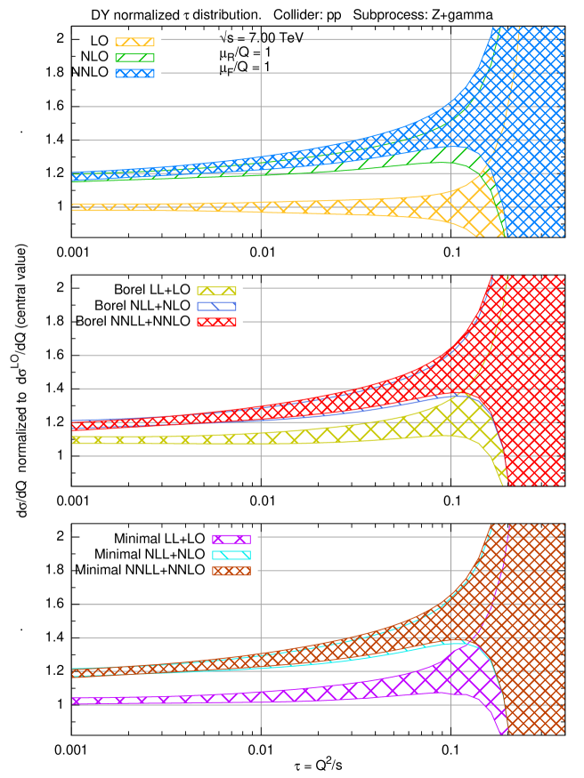
It ranges between 5% and 15% for . For larger values of the cross-section becomes essentially undetermined, because there are no data in PDF global fits to constrain PDFs in that region: the few available large– data are at much lower scale, and the uncertainty due to lack of information at very large contaminates PDFs down to when evolving up to the LHC scale. Note however that the Drell-Yan cross-section at large rapidly drops to unmeasurably small values (see Fig. 9). The fact that PDF uncertainties blow up for implies that data in this region would allow a determination of PDFs in a region where they are currently almost unknown; conversely, any signal of new physics in this region would have to be validated by measurements in an independent channel (such as for example jet production) which provides an independent constraint on the relevant PDFs.
In Fig. 11 we show the PDF uncertainties for the rapidity distribution of neutral Drell-Yan pairs with TeV at TeV, again using the NNPDF2.0 set with . As in the previous case, the PDF uncertainty does not depend significantly on the perturbative order, and it is typically larger than 5%.
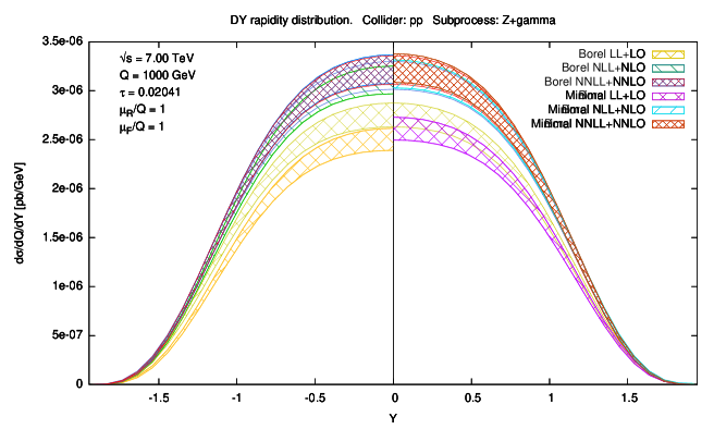
We now turn to the uncertainty due to the value of . The current PDG [39] value for is taken from Ref. [40] and it is . However, this uncertainty seems quite small, especially when taking into account the fluctuation in central values between the determinations that go into it, and the dependence on the perturbative order of some of them: indeed, current recommendations for precision LHC studies from the PDF4LHC group [38] advocate a rather more conservative uncertainty estimate. We thus take
| (5.2) |
as a reasonable current range.
The impact of this uncertainty on on the Drell-Yan cross-section at TeV can be estimated from Fig. 12,
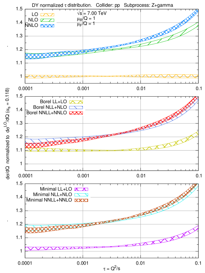
where we show the effect on the inclusive Drell-Yan cross-section due to variation in the range Eq. (5.2) of the value of used both in the computation of the hard matrix element and the PDF evolution. Results are only shown for , because for larger value the PDF uncertainty blows up and results loose significance, as discussed above. Note that this full dependence of the physical cross-section on is in general somewhat different from the dependence of the hard matrix element alone, because of the dependence on of the relevant parton luminosity. This total dependence might be larger or smaller according to whether the luminosity is correlated or anticorrelated to the value of , either of which might be the case for a quark luminosity, according to the kinematic region [8]. A priori, the size of the uncertainty due to variation of in the matrix element and that due to the dependence on of the PDFs are likely to be comparable: after all, the Drell-Yan rapidity distribution plays a significant role in the determination of the PDFs themselves.
It appears from Fig. 12 that the uncertainty increases with the perturbative order, but it is of similar size at the resummed and unresummed level; at NNLO it is of order of % at LHC energies; we have checked that it is about a factor two larger at Tevatron fixed-target experiments. The uncertainty due to on rapidity distributions is clearly of comparable size.
Noting that within the approximation of linear error propagation the PDF and uncertainties should be combined in quadrature [41], we conclude that PDF uncertainties are somewhat larger than uncertainties and the combined effect of PDF and uncertainties is likely to be smaller than about 10% but not much smaller, at least in the region in which PDFs are constrained by presently available data. Once PDF uncertainties will be reduced due to LHC data, it should be possible to keep the combined effect of these uncertainties at the level of few percent. Therefore, perturbative accuracies at the percent level are relevant for precision phenomenology.
5.3 Perturbative uncertainties: scale variations
A standard way of estimating unknown higher order perturbative corrections is to vary factorization and renormalization scales. We perform this variation by writing the factorized expression Eq. (2.7) as
| (5.3) |
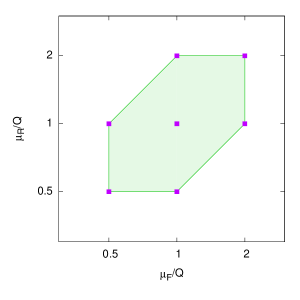
which is independent of and at the order at which the partonic coefficient is computed. The residual scale dependence is therefore of the first neglected order, and can be used as an estimate of the higher order terms in the perturbative expansion. We vary the two scales in the range
| (5.4) |
depicted in Fig. 13, which guarantees that both higher-order corrections to the partonic cross-section and to perturbative QCD evolution are generated, with the last condition ensuring that no artificially large scale ratios are introduced.
In the sequel, we will perform scale variation of both unresummed and resummed cross-sections. The interpretation of results deserves a comment. When performing scale variation of a result determined at fixed , one generates terms of : consequently, the scale uncertainty is reduced as one increases the perturbative order. However, terms generated by scale variation are proportional to those which are present at the given order: therefore, scale variation underestimates the size of higher order corrections when these are enhanced by higher logarithmic powers. For instance, scale variation of the Drell-Yan coefficient function Eq. (2.25) produces terms which at large grow at most as , whereas the actual coefficient function at large grows as . Hence, if is so large that these terms dominate the coefficient functions and must be resummed to all orders their impact might be rather larger than the scale variation of the fixed-order result may suggest. Nevertheless, in this case the scale dependence of the resummed result will still be smaller than that of the fixed-order result because the resummed result includes the dominant contributions to the cross-section to all orders.
However, in Sect. 2.3 we have seen that there is an intermediate kinematic region in which logarithmically enhanced contributions may provide a sizable fraction of the coefficient function even though : in this case, the resummation improves the fixed-order result in that it includes a sizable fraction of the higher order correction, but it still behaves in a perturbative way, i.e. terms of higher order in included through the resummation give an increasingly small contribution. If so, the scale dependence of the resummed result may well be comparable to or even larger than that of the fixed-order result, because the resummation amounts to the inclusion of large terms in the next few higher orders, which are not necessarily seen when performing the scale variation of the lower orders. Furthermore, resummation only affects the quark channel, while fixed-order scale variation mixes the quark and gluon channels: in an intermediate region, the logarithmic terms in the quark channel may be sizable, but with the gluon channel not being entirely negligible. In such case, the scale variation is dominated by subleading terms and thus we expect the residual scale dependence of the resummed result to differ according to the resummation prescription. We will see that this is indeed the case for resummation of Tevatron rapidity distributions, with scale variation of resummed results different according to whether the Borel or minimal prescription is used.
5.4 Tevatron at fixed target: NuSea
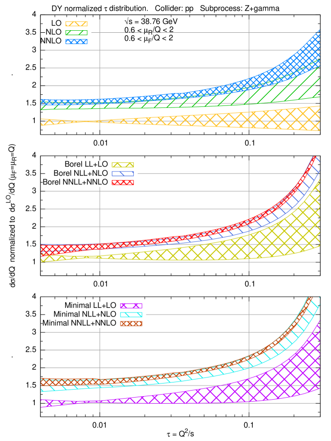
We begin by studying the invariant mass distribution of lepton pairs produced by collisions of a proton beam of energy GeV on a proton or deuteron target, at rest in the laboratory ( GeV). This is the experimental configuration of the experiment E866/NuSea. We first consider the inclusive invariant mass distribution. Results are shown in Fig. 14. All uncertainties shown here and henceforth are due to scale variation as described in Sect. 5.3. As expected, the width of the error bands decreases with increasing perturbative order. Note that for sufficiently small the uncertainty blows up, due to the fact that for fixed the small limit corresponds to low scale: for example, at this energy corresponds to GeV, and varying the scales as in Eq. (5.4) the values GeV are reached.
Turning now to the resummed results, we note that the numerical impact of resummation is large for , while for it is moderate but sill not negligible. Furthermore, starting with the NLL level, the scale uncertainty band for resummed results is dramatically smaller than in the case of fixed-order results. This is because scale variation of the LL result produces NLL terms which beyond the first few orders are not contained in the fixed-order result; starting with NLL these terms are already included in the resummed result. It is interesting to note that in the case of the resummed cross-section (with both prescriptions) the NNLL band is almost entirely contained in the NLL band, while the fixed-order NLO and NNLO error bands are only marginally compatible with each other. The ambiguity in the resummation, estimated from the difference between Borel and minimal prescription, is not negligible, but smaller than the scale uncertainty; moreover, it is more evident at small , since the different subleading terms give a larger contribution in that region.

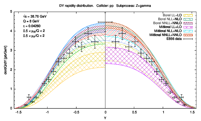
The experiment E866/NuSea [4] has measured the distribution in Eq. (4.5) of lepton pairs with an invariant mass GeV. The E866 data are displayed in Fig. 15, superimposed to the QCD prediction and the corresponding scale uncertainty. The distribution is symmetric about ; the curves shown for refer to fixed-order calculations, and those with to resummed results. The data agree with the NLO calculation because these data were included in the determination of the NLO PDFs that we are using.
The impact of the resummation is small but not negligible: for instance the difference between NNLO and NNLL is about half of the difference between NNLO and NLO. Furthermore, the scale uncertainty of resummed results is somewhat smaller than that of the unresummed ones. This is consistent with the observation that for this experiment , which, as discussed in Sect. 2, is in the region in which resummation is relevant. However, the difference between resummed results obtained using the Borel and the minimal prescription is almost as large as the size of the resummation itself: in fact the NLL Borel results is somewhat lower than the NNLO one, while the NLL minimal prescription result is a bit higher. Hence we conclude that the overall impact of the resummation on these data is essentially negligible. A large and negative NLL resummed correction to the NLO result was claimed in Ref. [6], using the minimal prescription, but we do not confirm it: we find a positive and rather smaller correction. The result of Ref. [6] was first criticized in Ref. [7]. Our result with the Borel prescription is in good quantitative agreement with Ref. [7]; however, the minimal prescription gives a somewhat larger correction, though still positive.
5.5 Tevatron collider
We now turn to Drell-Yan production in collisions at a center-of-mass energy TeV. Results for the invariant mass distribution of neutral and charged Drell-Yan pairs in this configuration are shown in Fig. 16.
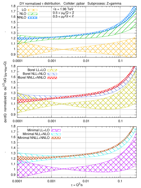
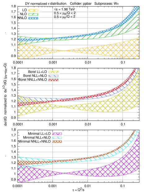
The behaviour of these curves is similar to that seen in the case of NuSea, Fig. 14, but with the impact of the resummation yet a bit smaller, as one would expect both because of the higher energy and because of the collider configuration, as discussed in Sect. 2.2 (in particular Fig. 3). Interestingly, even when the resummation has a very small impact, it still leads to a non-negligible reduction of the uncertainty: this is consistent with the expectation that for these medium-small values of resummation is in fact a perturbative correction, as discussed in the end of Sect. 2.3. Note that in these plots the smallness of leading-order uncertainty bands when (i.e. GeV2) is due to the fact that the scale dependence of the parton luminosity, to which the leading-order cross-section is proportional (see Eq. (4.11)), is stationary at this scale.
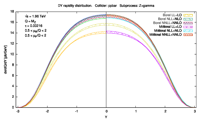


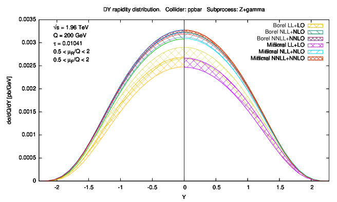
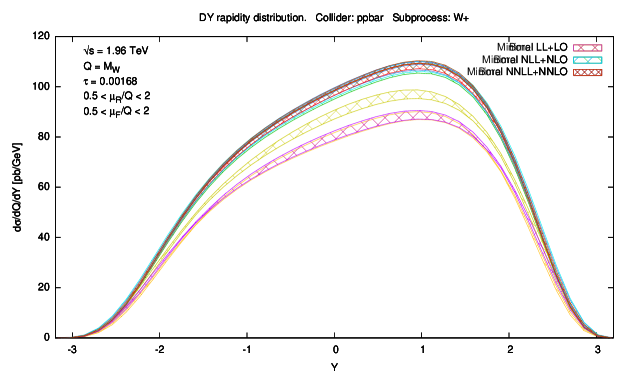


We now turn to rapidity distributions, shown in Figs. 17 and 18 for neutral Drell-Yan pairs of invariant mass and GeV respectively, and in Fig. 19 for charged Drell-Yan pairs of invariant mass . The impact of the resummation is now very small, as one would expect given the smallness of the relevant values of . However, interestingly, resummed uncertainty bands are systematically smaller than the unresummed one, with the resummation ambiguity (i.e. the difference between minimal and Borel results) now essentially negligible. Hence, even in this small region the resummation leads to perturbative improvement, while behaving of course as a perturbative correction. Again, note that the smallness of leading-order uncertainty bands is due to the fact that the scale here is close to the stationary point of the scale dependence of the parton luminosity already seen in Fig. 16.
We can compare these uncertainties to that of typical current data, thanks to recent measurements at the Tevatron. Specifically, the rapidity distribution of pairs with invariant mass in the range GeV GeV has been recently measured by the CDF collaboration [42]. In principle, the data should be compared with the theoretical prediction for the full process
| (5.5) |
For values of close to the mass, however, a good approximation is provided by the Breit-Wigner approximation, which amounts to assuming that the amplitude is dominated by exchange, and takes into account the finite width of the boson:
| (5.6) |
where is the decay width into a lepton pair, and is the differential cross-section for the production of a real on-shell boson. Eq. (5.6) gives
| (5.7) |
and therefore
| (5.8) |
where
| (5.9) |
is just a –independent multiplicative factor.
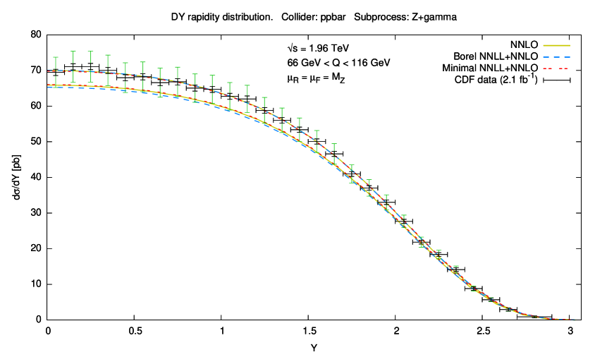
In Fig. 20 we show the CDF data [42], corresponding to an integrated luminosity of , compared to the NNLO QCD prediction with the inclusion of threshold resummation at NNLL, using both Borel and minimal prescriptions. The comparison shows an excellent agreement in shape between the data and the theoretical curves; there is clearly a mismatch in normalization of the total cross-section, which is however consistent with the sizable 6% normalization uncertainty on the cross-section. Also in this case, as for the NuSea experiment, this simply reflects the fact that these data are used in the determination of the PDFs that we are using, and the difference between the NLO expression used in PDF fitting and the NNLO one shown here is much smaller than the experimental uncertainties.
A similar comparison can be performed for the asymmetry, defined as
| (5.10) |
also measured by CDF [43]. In this case, normalization uncertainties cancel in the ratio. In Fig. 21 we show the measured CDF data [43] compared to the QCD prediction at NNLO and resummed NNLO+NNLL (Borel and minimal prescriptions).
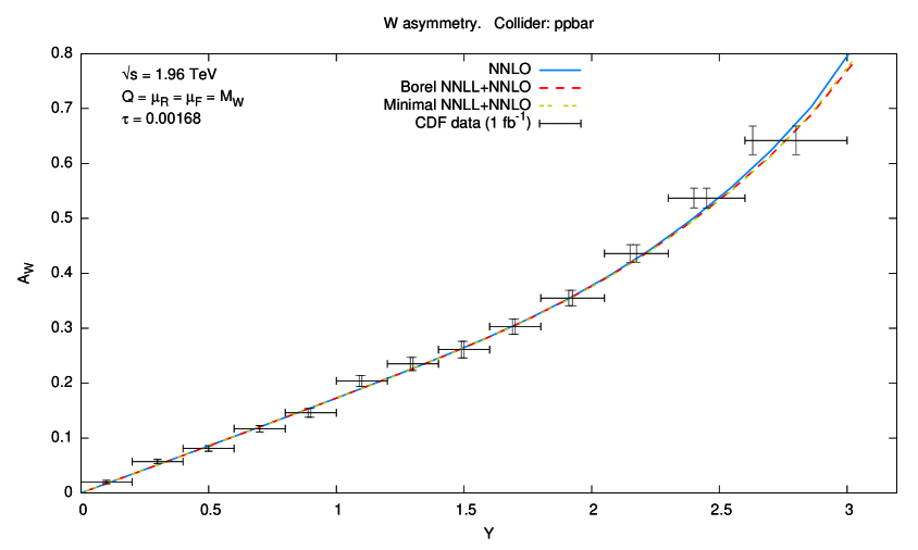
Clearly, the accuracy of present-day data is insufficient to appreciate the effect of NNLO or resummation correction, and it is rather comparable to the difference between LO and NLO predictions, which can thus be barely appreciated. However, an improvement of statistical accuracy by an order of magnitude would be sufficient for NNLO and resummation corrections to become significant. The normalization uncertainty has a negligible effect on the shape of the distribution and therefore it does not affect this conclusion
5.6 LHC
We now consider predictions for Drell-Yan production at the LHC, both at 7 TeV and 14 TeV. Invariant mass distributions for both neutral and charged Drell-Yan pairs are shown in Figs. 22, 23. While the impact of fixed-order perturbative corrections is unsurprisingly similar to that at the Tevatron collider shown in Fig. 16, interestingly the reduction in uncertainty obtained thanks to the resummation is more marked at the LHC, consistent with the expectation (recall Sect. 2) that the effect of the resummation is somewhat more significant at a than at a collider. Moreover, the consistency of the NLO error band with the NNLO prediction is improved by the inclusion of resummation. Of course, as in the case of Tevatron, for realistic values of the impact of the resummation is mostly on the uncertainty but very small or negligible on central values, so the resummation is behaving as a perturbative correction.
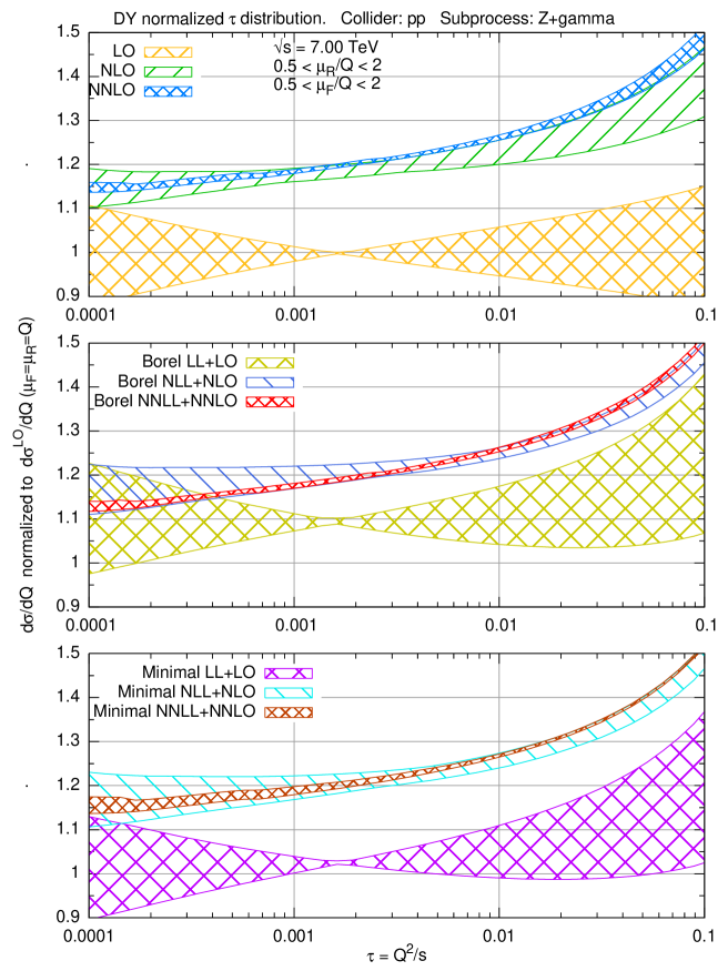

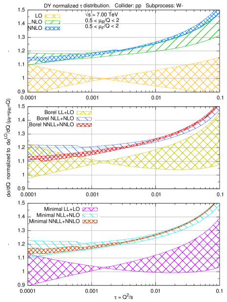
Turning to rapidity distributions, we present results for the following observables:
The first case corresponds to , comparable to the case of a final state with GeV at the Tevatron shown in Fig. 18. As in that case, we clearly see an improvement in uncertainty (with small resummation ambiguities) when going to the resummed result, though also in that case the effect on central value is moderate. On the other hand, the other cases correspond to very small values of and indeed in this case the uncertainty on resummed results is larger than that on unresummed ones, indicating that whatever effect is induced by the resummation is related to the inclusion of terms which are not dominant in this region. This is also reflected in a sizable difference between Borel and minimal results.
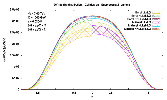


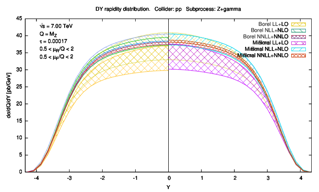
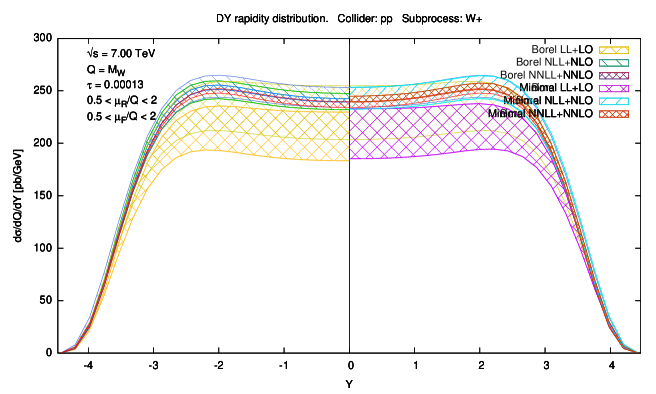

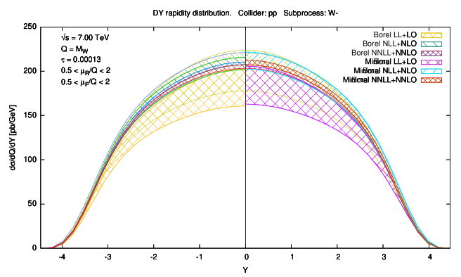

Finally, in Figs. 28–33 results for this same invariant mass and rapidity distributions for the LHC at 14 TeV are shown. The general behaviour is the same as that at the lower energy.
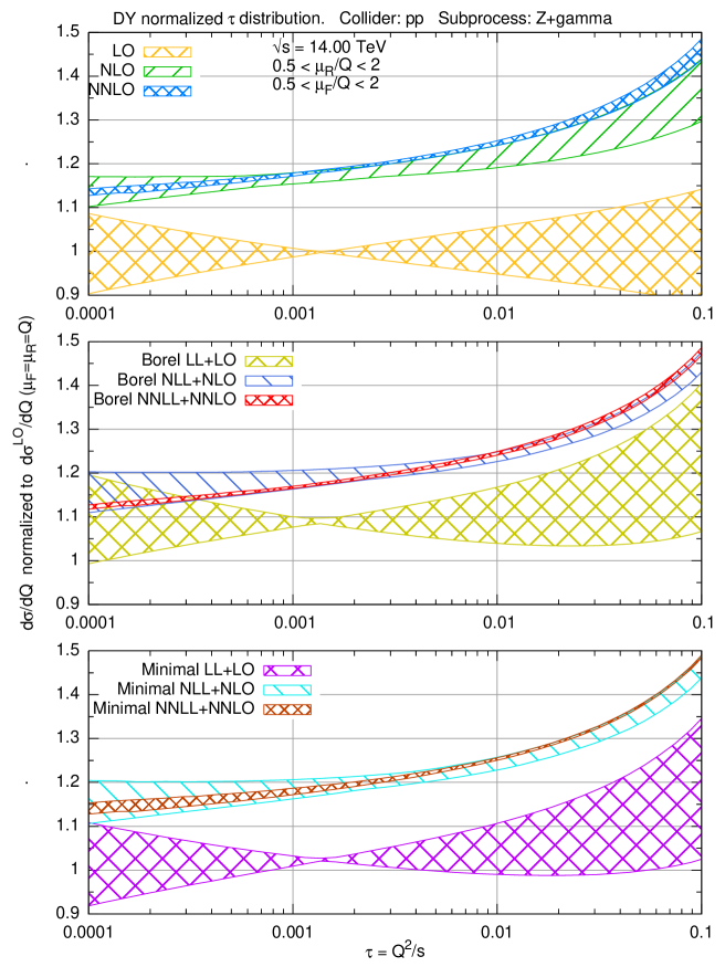
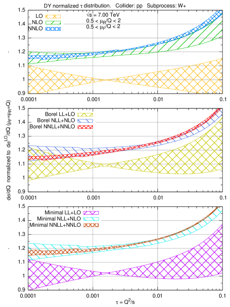


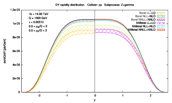

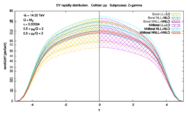
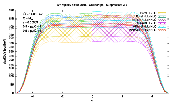

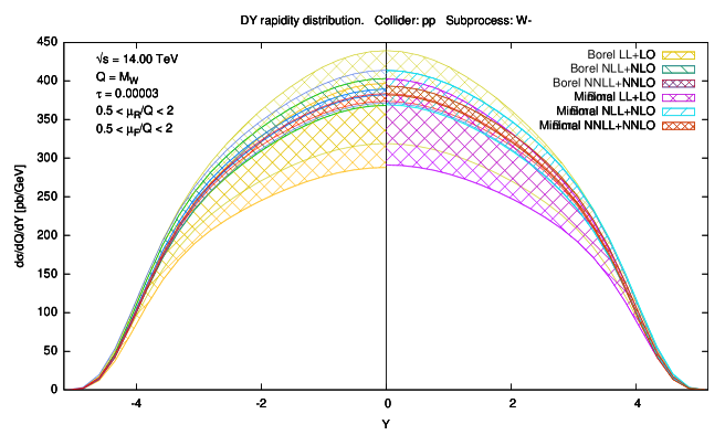

6 Conclusions
We have presented a discussion of the theory and phenomenology of threshold resummation of rapidity distributions, with special regard to present-day hadron colliders. On the theoretical side, our main result is that we have provided a way to estimate the value of at which resummation of threshold logarithms is expected to provide an improvement over fixed-order calculations. This result has been accomplished through a determination of the relevant partonic center-of-mass energy, whose distance from threshold determines the impact of resummation. This estimate relies on the singularity structure of the anomalous dimensions which drive evolution of parton distributions in perturbative QCD. Using this technique, we have shown that resummation is expected to be relevant down to fairly small values of at colliders, and at colliders.
At the phenomenological level, we have shown how to use different versions of the Borel resummation prescription and their comparison to the minimal prescription as a means to assess the ambiguities related to the resummation, and in particular to the treatment of the subleading terms. The application of these tools to the Tevatron and LHC has shown that resummation is relevant for the production of states of mass as light as and vector bosons at the Tevatron, and for the production of heavy dileptons of mass in the TeV range at the LHC: in all these cases threshold resummation leads to a significant improvement in perturbative accuracy. The impact of resummation on Tevatron fixed-target rapidity distributions is less clear, in that, despite being larger, the effect of resummation may be marred by its ambiguities.
Our general conclusion is that the impact of threshold resummation at hadron colliders for is comparable to that of NNLO corrections, and it should thus be included both in the determination of parton distributions and in precision phenomenology, though care should be taken in also estimating carefully the ambiguity which is intrinsic in the resummation procedure.
Acknowledgements: We thank M. Grazzini and A. Vicini for discussions and S. Catani for correspondence. This work was supported in part by the European network HEPTOOLS under contract MRTN-CT-2006-035505 and by an Italian PRIN-2008 grant.
Appendix A Saddle point
We collect here some results used in Sect. 2 on the saddle-point approximation to Mellin transform integrals of typical parton distributions.
First, we use the saddle-point method to show that the large– behaviour of a Mellin transform describes the original function of in the large– region. To see this, consider the Mellin transform of a generic function ,
| (A.1) |
we assume that in the range . For real, is a decreasing function of , because the area below the curve obviously decreases as increases.
The inverse Mellin transform is given by
| (A.2) |
with larger than the real part of the rightmost singularity of . We estimate the range of which gives the dominant contribution by saddle-point: we rewrite Eq. (A.2) as
| (A.3) |
where
| (A.4) |
For appropriate , as in the case of the physical cross-section, has a unique minimum on the real axis at , with
| (A.5) |
where a prime denotes differentiation with respect to . The inversion integral is dominated by the region of around , and can be approximated by
| (A.6) |
(after the variable change and gaussian integration). When , the slope of the straight line decreases, and the position of the minimum is pushed to larger values. We conclude that the behaviour of for close to 1 is determined by the large– behaviour of , as we set out to prove.
As an explicit example, we consider
| (A.7) |
with and positive constants. The function Eq. (A.7) vanishes both at and , and has a maximum at
| (A.8) |
which approaches as . We find
| (A.9) |
Let us now compute using the saddle-point approximation to invert the Mellin transform Eq. (A.9). We have
| (A.10) | |||
| (A.11) | |||
| (A.12) |
From Eq. (A.11) we find that the saddle point is at
| (A.13) |
which is, as expected, an increasing function of . Furthermore
| (A.14) | |||
| (A.15) |
Therefore, Eq. (A.6) gives
| (A.16) |
where
| (A.17) |
We see that the saddle-point approximation in this case gives the exact result, Eq. (A.7), up to a normalization factor, which however approaches 1 for large values of (the denominator of Eq. (A.17) is just in the Stirling approximation). Indeed, one can check that the Taylor expansion of to second order around is increasingly accurate as .
It is important to observe that the argument which shows that a Mellin transform Eq. (A.1) is a decreasing function of does not apply if in Eq. (A.2) is a distribution rather than an ordinary function. An obvious counter-example is the Dirac delta function, which has an –independent Mellin transform:
| (A.18) |
It is not difficult to find examples of distributions whose Mellin transforms even increase as increases. Let us consider for instance
| (A.19) |
where is a positive function, at most as singular as in . With the usual definition of the plus prescription, we have
| (A.20) |
which is finite under the above assumptions. The area below increases as increases, and therefore grows with .
In fact (see also Appendix B) this is the typical situation for the distributions , which characterize the large– and thus large– behaviour of soft-gluon emission cross-sections after the cancellation of infrared poles, and whose Mellin transforms behave as when . The coefficient of this logarithmic rise need not be positive, given that these are partonic cross-sections obtained after subtraction of infrared poles and factorization of collinear singularity.
Of course, the physical cross-section must be an ordinary function, so in the factorized expression Eq. (2.1) the decrease of the parton luminosity at large always offsets the increase of the partonic cross-section . Indeed, because the partonic cross-section rises at most as a power of as , it is easy to show that a sufficient condition for the Mellin inversion integral Eq. (2.5) of the factorized cross-section Eq. (2.1) to exist is that the parton luminosity vanishes at large at least as a positive power of .
Appendix B Mellin transformation
We collect here some results on the calculation of Mellin transforms of functions and distributions which typically appear in the perturbative coefficients. We start from the identity
| (B.1) |
(the plus prescription is not necessary if , but its presence makes the l.h.s. well defined even when ). It follows that
| (B.2) |
and therefore
| (B.3) |
with . Taking derivatives with respect to at we get
| (B.4) |
Note that the result Eq. (B.4) is a distribution, consistently with the fact that is an increasing function of . In other words, the inversion integral does not exist in the ordinary sense, but only in the sense of distributions.
An equivalent form of Eq. (B.4) is
| (B.5) |
where the integration contour is any closed curve in the complex plane with the origin inside. This form proves useful in the formulation of the Borel prescription for the Mellin inversion of divergent series in .
A second equivalent form of Eq. (B.4) is obtained by computing the derivative in the r.h.s. explicitly:
| (B.6) |
where
| (B.7) |
We see that the terms in the sum over are decreasingly important as .
Threshold logarithms typically appear in perturbative coefficients through the Mellin transform
| (B.8) |
We have
| (B.9) |
where
| (B.10) |
Hence
| (B.11) |
Appendix C Chebyshev polynomials
In this Appendix we recall the definition and the main properties of Chebyshev polynomials. The Chebyshev polynomials
| (C.1) |
are defined in the range recursively by
| (C.2a) | ||||
| (C.2b) | ||||
| (C.2c) | ||||
| (C.2d) | ||||
A generic function can be approximated in the range by its expansion on the basis of Chebyshev polynomials (C.2), truncated at some order :
| (C.3) |
where
| (C.4) |
Simple numerical algorithms for the calculation of the coefficients are available (we have used the routines of the gsl).
Simple algebra leads to
| (C.5) |
where
| (C.6) |
C.1 Minimal Prescription
We have shown in Sect. 3.1 that the minimal prescription can be conveniently implemented by means of an analytic expression for the Mellin transform of the luminosity (which can be either in the case of invariant mass distributions or in the case of rapidity distributions). This can be obtained by expanding on the basis of Chebyshev polynomials, truncated at some finite order , and then taking its analytical Mellin transform. The luminosity itself, however, is very badly behaved in the range : it is singular at , and varies by orders of magnitude in the range
| (C.7) |
It is therefore convenient to expand a regularized function
| (C.8) |
Values of and in the range are normally suited to make smooth enough to be approximated by a reasonably small number of Chebyshev polynomials. Equation (C.4) gives
| (C.9) |
and the approximation is
| (C.10) |
where
| (C.11) |
The luminosity is easily recovered:
| (C.12) |
where the last equality holds for integer. It is now immediate to obtain the Mellin transform:
| (C.13) |
Alternatively, one may introduce the variable
| (C.14) |
and appoximate the function
| (C.15) |
by an expansion on the basis of Chebyshev polynomials. The variable ranges from to 0 when ; however, for practical purposes one only needs the luminosity for . We have therefore
| (C.16) |
and
| (C.17) |
We can now reconstruct through the replacement . We get
| (C.18) |
The Mellin transform is computed using the result
| (C.19) |
We obtain
| (C.20) |
where
| (C.21) |
In practice, we have found that the second method is to be preferred for small values of , , while the previous one works better for .
C.2 Borel Prescription
In this case, we look for an approximation of the function , Eq. (4.49), as a function of . We have
| (C.22) |
where
| (C.23) |
and
| (C.24) |
Note that in this case. Therefore
| (C.25) |
In the case of the rapidity distributions, the variable is in the range ; therefore
| (C.26) |
Appendix D Resummed cross-section for the Drell-Yan process
In this Appendix we give the explicit expressions of the functions which appear in the resummed Drell-Yan cross-section, Eq. (3.2). We have [44]
| (D.1a) | ||||
| (D.1b) | ||||
| (D.1c) | ||||
| (D.1d) | ||||
with
| (D.2) |
The coefficients can be found in [45], but without scale-dependent terms. Their full expression is given by
| (D.3a) | ||||
| (D.3b) | ||||
The coefficients appearing in the previous functions are
| (D.4) | ||||
| (D.5) | ||||
| (D.6) | ||||
| (D.7) | ||||
| (D.8) | ||||
| (D.9) | ||||
| (D.10) |
D.1 Matching
Here we compute the terms to be subtracted in the resummed result in order to avoid double counting. Start from Eqs. (D.1) and expand them in powers of their argument :
| (D.11a) | ||||
| (D.11b) | ||||
| (D.11c) | ||||
The Taylor expansion of is
| (D.12) |
where (note that, since , it can be seen as an expansion in with fixed)
| (D.13) | ||||
| (D.14) |
References
- [1] C. Anastasiou, L. J. Dixon, K. Melnikov and F. Petriello, Phys. Rev. D 69 (2004) 094008 [arXiv:hep-ph/0312266].
- [2] S. Catani, G. Ferrera and M. Grazzini, JHEP 1005 (2010) 006 [arXiv:1002.3115 [hep-ph]].
- [3] M. Grazzini, arXiv:0908.1338 [hep-ph].
-
[4]
R. S. Towell et al. [FNAL E866/NuSea Collaboration],
Phys. Rev. D 64 (2001) 052002
[arXiv:hep-ex/0103030];
J. C. Webb, arXiv:hep-ex/0301031;
J. C. Webb et al. [NuSea Collaboration], arXiv:hep-ex/0302019. - [5] D. Appell, G. Sterman and P. B. Mackenzie, Nucl. Phys. B 309 (1988) 259.
- [6] P. Bolzoni, Phys. Lett. B 643 (2006) 325 [arXiv:hep-ph/0609073].
- [7] T. Becher, M. Neubert and G. Xu, JHEP 0807 (2008) 030 [arXiv:0710.0680 [hep-ph]].
- [8] R. D. Ball, L. Del Debbio, S. Forte, A. Guffanti, J. I. Latorre, J. Rojo and M. Ubiali, Nucl. Phys. B 838 (2010) 136 [arXiv:1002.4407 [hep-ph]].
- [9] M. Grazzini, PoS RADCOR2009 (2010) 047 [arXiv:1001.3766 [hep-ph]].
-
[10]
S. Catani, D. de Florian and M. Grazzini,
corrections at
JHEP 0105 (2001) 025
[arXiv:hep-ph/0102227];
S. Catani, D. De Florian and M. Grazzini, arXiv:hep-ph/0106049;
S. Catani, D. de Florian and M. Grazzini, JHEP 0201 (2002) 015 [arXiv:hep-ph/0111164];
S. Catani, D. de Florian, M. Grazzini and P. Nason, JHEP 0307 (2003) 028 [arXiv:hep-ph/0306211]. - [11] C. W. Bauer, N. D. Dunn and A. Hornig, arXiv:1010.0243 [hep-ph].
- [12] S. Catani, M. L. Mangano, P. Nason and L. Trentadue, Nucl. Phys. B 478 (1996) 273 [arXiv:hep-ph/9604351].
- [13] S. Forte, G. Ridolfi, J. Rojo and M. Ubiali, Phys. Lett. B 635 (2006) 313.
- [14] R. Abbate, S. Forte and G. Ridolfi, Phys. Lett. B 657 (2007) 55.
- [15] P.D.B. Collins, Introduction to Regge theory, Cambridge University Press (1977).
- [16] H. D. I. Abarbanel, M. L. Goldberger and S. B. Treiman, Phys. Rev. Lett. 22 (1969) 500.
- [17] See e.g. R. D. Ball et al. [NNPDF Collaboration], Nucl. Phys. B 809 (2009) 1 [Erratum-ibid. B 816 (2009) 293] [arXiv:0808.1231 [hep-ph]] and ref. therein.
- [18] R. K. Ellis, W. J. Stirling and B. R. Webber, “QCD and Collider Physics” (Cambridge, 1996)
- [19] G. Altarelli, R. K. Ellis and G. Martinelli, Nucl. Phys. B 143 (1978) 521 [Erratum-ibid. B 146 (1978) 544]; G. Altarelli, R. K. Ellis and G. Martinelli, Nucl. Phys. B 157 (1979) 461.
- [20] W. L. van Neerven and E. B. Zijlstra, Nucl. Phys. B 382 (1992) 11 [Erratum-ibid. B 680 (2004) 513].
- [21] G. F. Sterman, Nucl. Phys. B 281 (1987) 310.
- [22] S. Catani and L. Trentadue, Nucl. Phys. B 327 (1989) 323.
- [23] S. Forte and G. Ridolfi, Nucl. Phys. B 650 (2003) 229 [arXiv:hep-ph/0209154].
- [24] E. Laenen and G. F. Sterman, “Resummation for Drell-Yan differential distributions.” in Particles & Fields 92, published in DPF Conf.1992:987-989.
- [25] A. Mukherjee and W. Vogelsang, Phys. Rev. D 73 (2006) 074005 [arXiv:hep-ph/0601162].
- [26] H. Contopanagos, E. Laenen and G. F. Sterman, Nucl. Phys. B 484 (1997) 303 [arXiv:hep-ph/9604313].
- [27] S. Catani, Nucl. Phys. Proc. Suppl. 54A (1997) 107 [arXiv:hep-ph/9610413].
- [28] A. V. Manohar, Phys. Rev. D 68 (2003) 114019 [arXiv:hep-ph/0309176]; A. Idilbi and X. d. Ji, Phys. Rev. D 72 (2005) 054016 [arXiv:hep-ph/0501006];
- [29] T. Becher and M. Neubert, Phys. Rev. Lett. 97 (2006) 082001 [arXiv:hep-ph/0605050].
- [30] D. Bourilkov, R.C. Group and M.R. Whalley, hep-ph/0605240.
- [31] W. Furmanski and R. Petronzio, Nucl. Phys. B 195 (1982) 237.
- [32] A. D. Martin, W. J. Stirling, R. S. Thorne and G. Watt, Eur. Phys. J. C 63 (2009) 189 [arXiv:0901.0002 [hep-ph]].
- [33] H. L. Lai, M. Guzzi, J. Huston, Z. Li, P. M. Nadolsky, J. Pumplin and C. P. Yuan, arXiv:1007.2241 [hep-ph].
- [34] G. Balossini et al., JHEP 1001 (2010) 013 [arXiv:0907.0276 [hep-ph]].
- [35] http://www.ge.infn.it/bonvini/redy
- [36] http://www.slac.stanford.edu/lance/Vrap
- [37] S. Catani, L. Cieri, G. Ferrera, D. de Florian and M. Grazzini, Phys. Rev. Lett. 103 (2009) 082001 [arXiv:0903.2120 [hep-ph]].
- [38] https://wiki.terascale.de/index.php?title=PDF4LHC_WIKI
- [39] K. Nakamura et al. [Particle Data Group)]. J. Phys. G 37 (2010) 075021.
- [40] S. Bethke, Eur. Phys. J. C 64 (2009) 689 [arXiv:0908.1135 [hep-ph]].
- [41] H. L. Lai, J. Huston, Z. Li, P. Nadolsky, J. Pumplin, D. Stump and C. P. Yuan, arXiv:1004.4624 [hep-ph].
- [42] T. Aaltonen et al. [CDF Collaboration], arXiv:0908.3914 [hep-ex].
- [43] T. Aaltonen et al. [CDF Collaboration], Phys. Rev. Lett. 102 (2009) 181801 [arXiv:0901.2169 [hep-ex]].
- [44] S. Moch, J. A. M. Vermaseren and A. Vogt, Nucl. Phys. B 726 (2005) 317 [arXiv:hep-ph/0506288].
- [45] S. Moch and A. Vogt, Phys. Lett. B 631 (2005) 48 [arXiv:hep-ph/0508265].