Rejuvenating Power Spectra II: the Gaussianized galaxy density field
Abstract
We find that, even in the presence of discreteness noise, a Gaussianizing transform (producing a more-Gaussian one-point distribution) reduces nonlinearities in the power spectra of cosmological matter and galaxy density fields, in many cases drastically. Although Gaussianization does increase the effective shot noise, it also increases the power spectrum’s fidelity to the linear power spectrum on scales where the shot noise is negligible. Gaussianizing also increases the Fisher information in the power spectrum in all cases and resolutions, although the gains are smaller in redshift space than in real space. We also find that the gain in cumulative Fisher information from Gaussianizing peaks at a particular grid resolution that depends on the sampling level.
Subject headings:
cosmology: observations — large-scale structure of universe — methods: statistical1. Introduction
The power spectra of fluctuations in the matter and (more observably) galaxy fields carry important cosmological information. On large scales and early epochs, where the fluctuations are small and Gaussian, this information is preserved from early epochs, each Fourier mode having evolved linearly. On smaller scales, when the amplitudes of fluctuations grow to , the linear approximation breaks down. Modes of the overdensity become coupled, and their evolution becomes much harder to model. Inconveniently, we need high-order perturbation theory and numerical simulations to model the expectation value of the power spectrum accurately. A more fundamental problem is that the cosmic (co)variance in the power spectrum acquires a dominant non-Gaussian component on surprisingly large, “translinear” scales (Meiksin & White, 1999; Scoccimarro et al., 1999; Cooray & Hu, 2001). This has unpleasant consequences for cosmological parameter estimation, quantified by a “translinear plateau” in cumulative Fisher information content (Rimes & Hamilton, 2005, 2006; Neyrinck et al., 2006; Neyrinck & Szapudi, 2007; Lee & Pen, 2008; Takahashi et al., 2009).
Recently, we found that performing a logarithmic transform on the matter overdensity , i.e. using instead of as a density variable, drastically reduces the nonlinearities on translinear scales in the power spectrum (Neyrinck et al., 2009, Paper I). The logarithmic transform pushes the translinear plateau to scales about 2-3 times smaller, revealing about 10 times more Fisher information. It also gives a power-spectrum shape intriguingly close to the linear-theory prediction. The density field 1-point PDF (probability density function) is approximately lognormal (Coles & Jones, 1991); in fact, we found that an exact Gaussianization of the PDF (described below) performs even better.
PDF Gaussianization in large-scale structure was first proposed by Weinberg (1992), although not explicitly to increase power-spectrum information content, but to reconstruct the initial density field. Croft et al. (1998) used PDF Gaussianization in processing Lyman- forest data from quasar spectra, but this turns out not to be an essential step in estimating small-scale power spectra from this data, because radiative transfer already maps the overdensity into a narrow range of flux (Croft et al., 1999).
Although PDF Gaussianization impressively recovers the shape of the initial power spectrum, the transformation is less-successful in reconstructing initial mode-by-mode phases and amplitudes (Neyrinck et al., in prep). This is because of bulk motions of matter on Mpc scales, and formation of the cosmic web. For example, the initial and final PDF-Gaussianized fields shown in Fig. 1 in Paper I look by eye quite different on small scales. Precise reconstruction of the phases and amplitudes of translinear Fourier modes appears to require the accurate estimation and subtraction of the Lagrangian displacement field (e.g., Brenier et al., 2003; Eisenstein et al., 2007; Lavaux et al., 2008; Noh et al., 2009). With a Lagrangian reconstruction, it is obvious that the shape of the linear power spectrum should be reconstructed on translinear scales, but the methods are much more complicated and computationally intensive than a simple density PDF transform.
It does make sense intuitively that PDF Gaussianization should help the power spectrum to describe a field. While the cosmologically useful information in a Gaussian field is entirely in Fourier amplitudes, the information in a non-Gaussian field is partly in phase correlations, which are necessary to describe features such as sharp density peaks. Thus, flattening peaks restores information to the Fourier amplitudes from the phases. Phase correlations affect higher-order statistics, not the power spectrum, so Gaussianization can be seen as pulling information from higher-order statistics into the power spectrum.
In the approximation that a non-Gaussian field is a non-linear transformation of a Gaussian field, PDF Gaussianization will produce a Gaussian field, vanquishing all higher-order correlations. Conversely, subjecting a Gaussian field to a non-linear transformation produces higher-order correlations (Szalay, 1988). In particular, over length scales where the two-point correlation function is positive, a monotonic transformation will generally produce a positive four-point function, which indicates a positive non-Gaussian contribution to the covariance through the trispectrum. Thus it is plausible that much of the covariance on small scales is purely from the non-Gaussianity of the PDF. Perhaps a related statistic to the power spectrum of the Gaussianized field is the copula (Scherrer et al., 2010), which is similarly immune to monotonic transformations on the field it is applied to.
Despite the promising results, there remain issues to be resolved before PDF Gaussianization can be used in practice. In this paper, we investigate discreteness noise. For a logarithmic transform, the problem becomes obvious when there are cells with zero galaxies, which would transform to . We first investigate the ideal case of Poisson noise in the matter power spectrum, and then the galaxy power spectrum. We also make a start at exploring the effect of redshift distortions.
2. Gaussianizing transformations
There are many possible meanings of “Gaussianizing.” For example, Zhang et al. (2010) split a density field into Gaussianized and non-Gaussianized components based on distributions of wavelet coefficients, and showed that the Gaussianized component of the matter density field carries somewhat more Fisher information than the full field. In the present paper, by “Gaussianization” we mean PDF Gaussianization, i.e. a function applied equally to each pixel that reduces the higher-order moments of the one-point distribution of the field.
We use a simple approach, first estimating the density using simple Nearest-Grid-Point (NGP) mass assignment, and then Gaussianizing. Perhaps some gains in information on small scales could come from using a higher-order mass assignment scheme, or an interpolation naturally suited to discrete data, for example the DTFE (Delaunay Tessellation Field Estimator, van de Weygaert & Schaap, 2009). Sophisticated techniques have even been developed to estimate the field directly (e.g., Kitaura et al., 2010; Weig & Enßlin, 2010). Here we choose NGP for its simplicity, and for the simple, constant form of its shot noise, at least for ideal Poisson data. More-sophisticated techniques could perform (or inform) even better.
The two transformations we consider are “exact” Gaussianization, , and a modified logarithmic transform, . Seo et al. (2010) have dealt with the problem of log-transforming zero cells by introducing a density floor, i.e. adding an arbitrary small, positive parameter to the argument of the logarithm. This alternative modified logarithmic transform did succeed in boosting the Fisher information in the lensing-convergence power spectrum. There are many possible alternative Gaussianizing transforms. One commonly used transform used for producing a Gaussian distribution from a Poisson distribution is the Anscombe (1948) transform, but this transform is not ideal in our case. While the separate density PDF’s for each pixel, over different realizations, should be Poisson in our case, the global pixel density PDF will generally not be Poisson.
Our first transformation, , is the density one would expect from an exactly Gaussian PDF with the same ranking of cell densities as . Explicitly,
| (1) |
where is the fraction of cells less-dense than in the density field, is the standard deviation of the Gaussian that is mapped onto, and is the number of cells. If there are multiple cells with the same , as usually occurs in Poisson-sampled ’s, then there will be some range of that is mapped to cells with the same . In this case, the actual that we assign to these cells is an average of over this range.
On the other hand, a drawback of is that it is globally defined, nontrivially depending on the entire field. Also, the implicitly defined function need not be well-behaved, complicating attempts at predicting statistics of analytically. So, we also investigate a modified logarithmic transform, which only depends globally on through the mean density. We define
| (2) |
3. Poisson-sampled matter density fields
First we investigate the simple case of exact Poisson discreteness noise, in the matter field investigated in Paper I. We Poisson-sample the density field of the Millennium Simulation (MS, Springel et al., 2005) on a publicly available density grid at , at various sampling levels, from to particles per (2 Mpc)3 cell. (The full sampling level of the MS is .) To Poisson-sample, we simply set the number of particles in a cell to a random Poisson number of mean equal to the full-sampling density.
3.1. Effects on the mean
It is well-known (e.g., Peebles, 1980) that particle discreteness produces a white-noise shot noise in the power spectrum, where is the number density of particles.
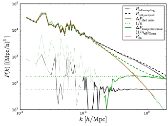
Fig. 1 shows shot noises of and , estimated as the difference between power spectra of the density fields with and without the added discreteness noise, measured from the MS matter density field on a grid. When and (the power spectra of and ) are plotted in this paper, we multiply them by constants to line them up with in the lowest- bin. For , this is equivalent to setting the used in Eq. (1).
For , as expected, the simple estimate works quite well. The shot noise in , on the other hand, carries some slight scale dependence, and is generally greater than the shot noise. Intuitively, Gaussianization increases the shot noise because it increases the contrast between low-density cells.
The green dot-dashed curve in Fig. 1 shows an estimate of this shot noise. It was calculated from a histogram of , using the empirical expression
| (3) |
substituting for . Here, is the volume of a cell, and is the fraction of cells with , for density bins .
Eq. (3) is motivated by the low-density tail of the density distribution, where the function stretches the contrast. For example, in a density field with cells of only 0 or 1 particle, . When this density field is transformed by , the shot noise increases, proportionally with . A simpler approximation than Eq. (3) would be to use only in the sum (as in the preceding example), but we found that Eq. (3) works a bit better.
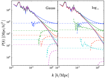
Fig. 2 explores the shot noise in and with varying sampling levels on a grid. The shot noise in at high sampling and high is generally smaller than in ; however, the shape of ’s shot-noise curve is less consistent than ’s. This hints at the higher (co)variance in than in , which will be discussed further in the next subsection. The estimate in Eq. (3) works well for low sampling, but overestimates the shot noise if the sampling is , especially in the case.
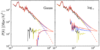
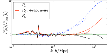
Fig. 3 shows how the shot noise varies with resolution, at a fixed sampling. Generally, especially for , the shot noise is rather consistent for different resolutions. In fact, the approximation that the shot noise is constant over different resolutions seems to be a better approximation than the one in Eq. (3), so we will use it when we deal with galaxies (with no easily measurable “no-shot-noise” power spectrum).
The bottom panel of Fig. 3 shows the “nonlinear transfer function” for , raw and after subtracting shot noise, and for (after subtracting shot noise).
3.2. Effects on Information Content
As in Paper I, we use a Fisher information (Fisher, 1935; Tegmark et al., 1997) formalism to quantify the information in the power spectrum. The cumulative Fisher information in the power spectrum about parameters and over a range of power-spectrum bin indices is estimated as
| (4) |
where is the square submatrix of C with both indices ranging over . is the covariance matrix of the power spectrum in bins, .
In Paper I, we considered the signal-to-noise ratio S/N, the information in the power spectrum about the power spectrum itself. (S/N)2 (called simply S/N in Paper I) is the Fisher information about a (possibly hypothetical) parameter that depends on each mode of the power spectrum equally. Thus, the derivative terms above were set to unity. For , the linear-power-spectrum amplitude (e.g., investigated in Rimes & Hamilton, 2005; Neyrinck et al., 2006) is a parameter such that on linear scales, reaching on translinear scales. The situation is more subtle in the case of power spectra of nonlinearly-transformed fields, since there is generally a large-scale bias (Paper I). But this does not affect parameters that depend on the power spectrum’s shape. And for parameters that depend on the amplitude, the large-scale bias can be constrained by measuring both and (or ) in the linear regime. In this paper, though, we simply investigate the S/N in (and ) themselves. This would be entirely appropriate when comparing data to a mock catalog, for example.
Shot noise further complicates the situation. The statistically stable shot noise component of the power spectrum that appears on small scales actually reduces the covariance in (the power spectrum including shot noise), mimicking a gain in clustering information, when really all that’s being accurately measured is the shot noise. The correct thing to investigate is the information in about the power spectrum without shot noise, . Thus we investigate
| (5) | |||||
For the last line, we assume that the shot noise is independent of the clustering fluctuations. In fact, this result is roughly what one would get by subtracting the mean shot noise from the power spectra before measuring the covariance matrix. For example, if the covariance matrix is diagonal, the Fisher-matrix entries for the power spectrum including shot noise will be . Plugging this into Eq. (5) causes the fractions to cancel, giving the Fisher-matrix entries for the power spectrum without shot noise.
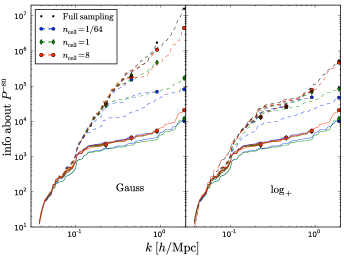
Fig. 4 shows a comparison of the (S/N)2 in , , and , for Poisson-sampled density fields of various resolutions and samplings of the MS. As in Paper I, covariance matrices are estimated from power spectra measured after applying 248 sinusoidal weightings (Hamilton et al., 2006) to the density field. (dashed) out-informs (solid) in all cases, although the gains are modest at a sampling of .
Interestingly, especially for , there appears to be a resolution at which the gains in information from Gaussianization (i.e. the vertical distance between the dashed and solid curves) peak. This is not surprising: in the low-resolution limit, the field is already Gaussian, so Gaussianization has no effect. In the high-resolution limit, even the highest peaks can only be sampled with one particle, giving a field of only 0’s and 1’s, which Gaussianization will only cause to be multiplied by a constant. Mathematically, the information without the fractions keeps rising, but these fractions can cause it to turn over, producing a peak. As we find below in Section 4.2, the peak is generally at a resoution a few times coarser than that where . And particularly if one is interested in the power spectrum over the range of scales just smaller than the linear regime (( Mpc-1) ), and not in scraping information from smaller scales, it is wise to Gaussianize at this peak resolution or coarser.
4. Galaxy density fields
In this section, we address the impacts of discreteness and redshift-space distortions on the observationally relevant case of a galaxy density field, in both real and redshift space. Again we use the MS, using the publicly available galaxy catalog as modelled by De Lucia & Blaizot (2007). We use three galaxy samples, with R-band absolute-magnitude cuts , , and ; these have respective mean galaxy number densities of about , 0.02, and 0.1 ( Mpc)-3. We generate galaxy-density grids using NGP density assignment from these galaxy samples. A tiny fraction of galaxies exactly overlapped other galaxies in position; in this case, we keep only the brightest one. In the redshift-space case, before gridding the galaxies we first displace them along the -axis by .
4.1. Effects on the mean
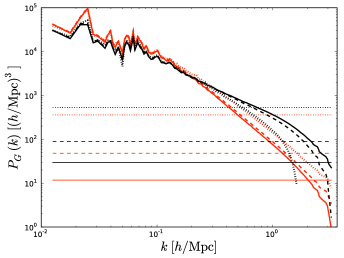
Fig. 5 shows for galaxy density fields using the , , and samples, in real and redshift space. In each case, we have subtracted a shot noise, constant in , and shown with faint lines. In this subsection we do not show because its shape in all cases is nearly identical to . As in the matter power spectrum section, in showing , we set the variance of the Gaussians onto which the ’s are mapped so that the power spectra line up in the lowest bin.
In the matter case, the shot noise could be directly measured by comparing to a very well-sampled matter density field, which we lack in the galaxy case. We estimate the shot noise using a prescription motivated by the rough agreement of the shot noise across different resolutions in Fig. 2. We measure the power spectrum on a rather high-resolution () grid, and assume that for all resolutions, the shot noise is a constant with , at an amplitude of . (Here, is the highest measured in the high-resolution grid. pIn the cubic box, , although we only plot the power spectra to .) This probably overestimates the shot noise somewhat, but perhaps this is appropriate, at least for , given the slight rise in the shot-noise power at slightly lower than (e.g., at Mpc-1 in Fig. 2).
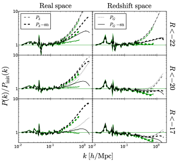
Fig. 6 shows ratios of galaxy power spectra to the linear power spectrum , in both real and redshift space. These could be thought of as transfer functions between and galaxy power spectra.
In real space, in the limit of low sampling (in the sample), and look nearly identical before shot noise is subtracted. This is not surprising, as differs not much, after removing a linear scaling, from in this limit. But after shot noise is subtracted, even at this sampling, seems to track a bit better than . As the sampling increases (in the sample), comes to track significantly better, even before shot noise is subtracted.
In redshift space, the story is not as clear. A full analysis of the effects of redshift-space distortions on is beyond the scope of this paper. One obvious piece of analysis that is lacking is that here we merely analyze the angle-averaged redshift-space power spectrum. But in general, Gaussianization modifies the shape of galaxy power spectra less in redshift space than in real space. This is likely because the galaxy-density PDF is already somewhat Gaussianized because peaks are smeared by fingers of God.
4.2. Effects on Information Content
Our method in investigating the galaxy power spectrum Fisher information, (S/N)2, is essentially the same as in the matter case. The difference is that we do not have a meaningful measurement of the exact shot noise, and so we estimate it as in Section 4.1. This estimate is conservative (i.e. likely an overestimate) from the point of view of information estimation, so the information curves for and appearing below could be considered conservative at high (i.e. perhaps a slight underestimate). For , we use the simple factor.
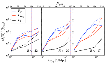
Fig. 7 shows (S/N)2() curves for the real-space power spectra , , and , for the three MS galaxy samples, measured on grid sizes varying from to . To reduce clutter, we do not show each cumulative (S/N)2 curve, but just the total cumulative (S/N)2() up to the Nyquist frequency . In the matter case (Fig. 4), these appear as symbols at information-curve endpoints. The dashed lines show (S/N)2 without taking into account shot noise [i.e. without the fractions in Eq. (5)]. The solid lines, for which these fractions are included, are more meaningful.
Typically, as suggested in the matter case in Fig. 4, there appears to be a peak in the gain in (S/N)2( provided by the Gaussianization transform. The dotted lines are at the resolution where the shot noise is most comparable to the clustering signal; here, there is typically a trough in the cumulative (S/N)2. It appears that the resolution that optimizes the gain from Gaussianizing is typically a factor of 2-4 coarser than that. But in all cases, the Gaussianized power spectra out-inform the standard power spectra.
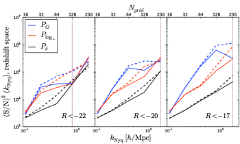
Fig. 8 shows the same for redshift-space power spectra. Here, fares better, likely because in redshift space, fingers of God smear out density peaks and already make the PDF of more Gaussian. Still, again the power spectra of the Gaussianized fields out-inform in all cases.
5. Conclusion
In this paper, we extend our previous analysis of the rejuvenating effects that PDF Gaussianization has on the matter power spectrum (Paper I). We include discreteness effects, and look at the observationally relevant case of the galaxy density field, both in real and redshift space. As in Paper I, we analyze the Millennium Simulation.
We find that the conclusions of Paper I remain unchanged in the presence of discreteness noise, as long as one is looking at scales where the shot noise (which Gaussianization does increase somewhat) is negligible. In real space, Gaussianizing the galaxy and discretized matter density fields does seem to extend the range over which their power spectra trace the linear power spectrum, well into the nonlinear regime, until the shot noise becomes comparable to the clustering signal. In redshift space, Gaussianization also reduces the small-scale rise in the galaxy power spectrum.
Gaussianization removes or reduces the small-scale rise that one sees in power spectra relative to the linear power spectrum. In the context of the halo model (e.g., Cooray & Sheth, 2002), this rise is associated with a one-halo term. It is perhaps not surprising that Gaussianizing would reduce this one-halo term, since haloes are the most non-linear, non-Gaussian structures in the Universe. However, the removal of this rise in the galaxy power spectrum without direct mention of haloes also suggests that explaining galaxy bias with a non-linear transformation of a Gaussian field (e.g., Politzer & Wise, 1984; Szalay, 1988), which has somewhat gone out of fashion, may be a fruitful area for further study.
In all cases, Gaussianization also improves the inherent Fisher information, (S/N)2, of the power spectrum. But the degree of help it provides depends on the resolution of the grid over which the PDF is Gaussianized. It seems that the grid size providing the most cumulative added (S/N)2 is a factor of 2-4 coarser than the resolution where, at the grid’s Nyquist frequency, the shot noise and clustering components of the power spectrum are of comparable magnitude. That is, to reap the information gains of Gaussianization on translinear scales, one should be careful not to use grid cells that are too small. In redshift space, the gains in (S/N)2 for galaxy density fields are somewhat smaller than in real space, if the galaxy sampling is high enough to resolve fingers of God. This is because fingers of God smear high density peaks, producing an already more-Gaussian PDF.
While discreteness effects are an essential issue to investigate in the study of power spectra of Gaussianized fields, a few issues still remain. With a variable survey selection function, it may be necessary to apply a Gaussianization transform seperately in different redshift shells. We have made a start at analyzing the effects of redshift distortions, but much more work can be done in this area. It also remains to be investigated precisely how faithfully, and to what scales, the power spectrum of the Gaussianized matter and galaxy density fields traces the linear power spectrum, for arbitrary cosmologies. Put more practically, the Fisher-matrix analysis needs to be extended to particular cosmological parameters. Also, our assertion that Gaussianization pulls information from higher-point statistics could do with further quantitative elucidation.
References
- Anscombe (1948) Anscombe, F. J. 1948, Biometrika, 35, 246
- Brenier et al. (2003) Brenier, Y., Frisch, U., Hénon, M., Loeper, G., Matarrese, S., Mohayaee, R., & Sobolevskiĭ, A. 2003, MNRAS, 346, 501, arXiv:astro-ph/0304214
- Coles & Jones (1991) Coles, P., & Jones, B. 1991, MNRAS, 248, 1
- Cooray & Hu (2001) Cooray, A., & Hu, W. 2001, ApJ, 554, 56, arXiv:astro-ph/0012087
- Cooray & Sheth (2002) Cooray, A., & Sheth, R. 2002, Phys. Rep., 372, 1, arXiv:astro-ph/0206508
- Croft et al. (1998) Croft, R. A. C., Weinberg, D. H., Katz, N., & Hernquist, L. 1998, ApJ, 495, 44, arXiv:astro-ph/9708018
- Croft et al. (1999) Croft, R. A. C., Weinberg, D. H., Pettini, M., Hernquist, L., & Katz, N. 1999, ApJ, 520, 1, arXiv:astro-ph/9809401
- De Lucia & Blaizot (2007) De Lucia, G., & Blaizot, J. 2007, MNRAS, 375, 2, arXiv:astro-ph/0606519
- Eisenstein et al. (2007) Eisenstein, D. J., Seo, H., Sirko, E., & Spergel, D. N. 2007, ApJ, 664, 675, arXiv:astro-ph/0604362
- Fisher (1935) Fisher, R. A. 1935, J. Roy. Stat. Soc., 98, 39
- Hamilton et al. (2006) Hamilton, A. J. S., Rimes, C. D., & Scoccimarro, R. 2006, MNRAS, 371, 1188, arXiv:astro-ph/0511416
- Kitaura et al. (2010) Kitaura, F., Jasche, J., & Metcalf, R. B. 2010, MNRAS, 403, 589, 0911.1407
- Lavaux et al. (2008) Lavaux, G., Mohayaee, R., Colombi, S., Tully, R. B., Bernardeau, F., & Silk, J. 2008, MNRAS, 383, 1292, 0707.3483
- Lee & Pen (2008) Lee, J., & Pen, U.-L. 2008, ApJ, 686, L1, arXiv:0807.1538
- Meiksin & White (1999) Meiksin, A., & White, M. 1999, MNRAS, 308, 1179, arXiv:astro-ph/9812129
- Neyrinck & Szapudi (2007) Neyrinck, M. C., & Szapudi, I. 2007, MNRAS, 375, L51, arXiv:astro-ph/0610211
- Neyrinck et al. (2006) Neyrinck, M. C., Szapudi, I., & Rimes, C. D. 2006, MNRAS, 370, L66, arXiv:astro-ph/0604282
- Neyrinck et al. (2009) Neyrinck, M. C., Szapudi, I., & Szalay, A. S. 2009, ApJ, 698, L90, 0903.4693 (Paper I)
- Neyrinck et al. (in prep) ——. in prep
- Noh et al. (2009) Noh, Y., White, M., & Padmanabhan, N. 2009, Phys. Rev. D, 80, 123501, 0909.1802
- Peebles (1980) Peebles, P. J. E. 1980, The large-scale structure of the universe (Princeton, N.J., Princeton University Press, 1980. 435 p.)
- Politzer & Wise (1984) Politzer, H. D., & Wise, M. B. 1984, ApJ, 285, L1
- Rimes & Hamilton (2005) Rimes, C. D., & Hamilton, A. J. S. 2005, MNRAS, 360, L82, arXiv:astro-ph/0502081
- Rimes & Hamilton (2006) ——. 2006, MNRAS, 371, 1205, arXiv:astro-ph/0511418
- Scherrer et al. (2010) Scherrer, R. J., Berlind, A. A., Mao, Q., & McBride, C. K. 2010, ApJ, 708, L9, 0909.5187
- Scoccimarro et al. (1999) Scoccimarro, R., Zaldarriaga, M., & Hui, L. 1999, ApJ, 527, 1, arXiv:astro-ph/9901099
- Seo et al. (2010) Seo, H., Sato, M., Dodelson, S., Jain, B., & Takada, M. 2010, ArXiv e-prints, 1008.0349
- Springel et al. (2005) Springel, V. et al. 2005, Nature, 435, 629, arXiv:astro-ph/0504097
- Szalay (1988) Szalay, A. S. 1988, ApJ, 333, 21
- Takahashi et al. (2009) Takahashi, R. et al. 2009, ApJ, sumbitted, arXiv:0902.0371
- Tegmark et al. (1997) Tegmark, M., Taylor, A. N., & Heavens, A. F. 1997, ApJ, 480, 22, arXiv:astro-ph/9603021
- van de Weygaert & Schaap (2009) van de Weygaert, R., & Schaap, W. 2009, in Data Analysis in Cosmology, ed. V. Martinez, E. Saar, E. Martínez-Gonzáles, & M.-J. Pons-Bordería (Berlin: Springer), arXiv:0708.1441
- Weig & Enßlin (2010) Weig, C., & Enßlin, T. A. 2010, MNRAS, 409, 1393, 1003.1311
- Weinberg (1992) Weinberg, D. H. 1992, MNRAS, 254, 315
- Zhang et al. (2010) Zhang, T., Yu, H., Harnois-Déraps, J., MacDonald, I., & Pen, U. 2010, ArXiv e-prints, 1008.3506