Robust Shrinkage Estimation of High-dimensional Covariance Matrices
Abstract
We address high dimensional covariance estimation for elliptical distributed samples, which are also known as spherically invariant random vectors (SIRV) or compound-Gaussian processes. Specifically we consider shrinkage methods that are suitable for high dimensional problems with a small number of samples (large small ). We start from a classical robust covariance estimator [Tyler(1987)], which is distribution-free within the family of elliptical distribution but inapplicable when . Using a shrinkage coefficient, we regularize Tyler’s fixed point iterations. We prove that, for all and , the proposed fixed point iterations converge to a unique limit regardless of the initial condition. Next, we propose a simple, closed-form and data dependent choice for the shrinkage coefficient, which is based on a minimum mean squared error framework. Simulations demonstrate that the proposed method achieves low estimation error and is robust to heavy-tailed samples. Finally, as a real world application we demonstrate the performance of the proposed technique in the context of activity/intrusion detection using a wireless sensor network.
Index Terms:
Covariance estimation, large small , shrinkage methods, robust estimation, elliptical distribution, activity/intrusion detection, wireless sensor networkI Introduction
Estimating a covariance matrix (or a dispersion matrix) is a fundamental problem in statistical signal processing. Many techniques for detection and estimation rely on accurate estimation of the true covariance. In recent years, estimating a high dimensional covariance matrix under small sample size has attracted considerable attention. In these “large small ” problems, the classical sample covariance suffers from a systematically distorted eigen-structure [Jonestone], and improved estimators are required.
Much effort has been devoted to high-dimensional covariance estimation, which use Steinian shrinkage [Stein, Ledoit2004, Chen] or other types of regularized methods such as [Bickel-Levina06, graph-lasso]. However, most of the high-dimensional estimators assume Gaussian distributed samples. This limits their usage in many important applications involving non-Gaussian and heavy-tailed samples. One exception is the Ledoit-Wolf estimator [Ledoit2004], where the authors shrink the sample covariance towards a scaled identity matrix and proposed a shrinkage coefficient which is asymptotically optimal for any distribution. However, as the Ledoit-Wolf estimator operates on the sample covariance, it is inappropriate for heavy tailed non-Gaussian distributions. On the other hand, traditional robust covariance estimators [Huber81, Tyler87, Rousseeuw85] designed for non-Gaussian samples generally require and are not suitable for “large small ” problems. Therefore, the goal of our work is to develop a covariance estimator for problems that are both high dimensional and non-Gaussian. In this paper, we model the samples using the elliptical distribution [Kelker], which is also referred to as the spherically invariant random vector model (SIRV) [Yao, Yao04] or the compound-Gaussian process model [Conte1995]. As a flexible and popular alternative, the elliptical family encompasses a large number of important distributions such as Gaussian distribution, the multivariate Cauchy distribution, the multivariate exponential distribution, the multivariate Student-T distribution, the K-distribution and the Weibull distribution. The capability of modelling heavy-tails makes the elliptical distribution appealing in signal processing and related fields. Typical applications include radar detection [MIT, Conte1995, Rangaswamy05, Wang], speech signal processing [Brehm87], remote sensing [Vasile], wireless fading channels modelling [Yao04], financial engineering [Frahm2004] and so forth.
A well-studied covariance estimator for elliptical distributions is the ML estimator based on normalized samples [Tyler87, Gini02, Conte02]. The estimator is derived as the solution to a fixed point equation by using fixed point iterations. It is distribution-free within the class of elliptical distributions and its performance advantages are well known in the regime. However, it is not suitable for the “large small ” setting. Indeed, when , the ML estimator as defined does not even exist. To avoid this problem the authors of [Abrmovich] propose an iterative regularized ML estimator that employs diagonal loading and uses a heuristic procedure for selecting the regularization parameter. While they did not establish convergence and uniqueness [Abrmovich] they empirically demonstrated that their algorithm has superior performance in the context of a radar application. Our approach is similar to [Abrmovich] but we propose a systematic procedure of selecting the regularization parameter and establish convergence and uniqueness of the resultant iterative estimator. Specifically, we consider a shrinkage estimator that regularizes the fixed point iterations. For a fixed shrinkage coefficient, we prove that the regularized fixed iterations converge to a unique solution for all and , regardless of the initial condition. Next, following Ledoit-Wolf [Ledoit2004], we provide a simple closed-form expression for the shrinkage coefficient, based on minimizing mean-squared-error. The resultant coefficient is a function of the unknown true covariance and cannot be implemented in practice. Instead, we develop a data-dependent “plug-in” estimator approximation. Simulation results demonstrate that our estimator achieves superior performance for samples distributed within the elliptical family. Furthermore, for the case that the samples are truly Gaussian, we report very little performance degradation with respect to the shrinkage estimators designed specifically for Gaussian samples [Chen].
As a real world application we demonstrate the proposed estimator for activity/intrusion detection using an active wireless sensor network. We show that the measured data exhibit strong non-Gaussian behavior and demonstrate significant performance advantages of the proposed robust covariance estimator when used in a covariance-based anomaly detection algorithm.
The paper is organized as follows. Section II provides a brief review of elliptical distributions and of Tyler’s covariance estimation method. The regularized covariance estimator is introduced and derived in Section III. We provide simulations and experimental results in Section IV and Section V, respectively. Section VI summarizes our principal conclusions. The proof of theorems and lemmas are provided in the Appendix.
Notations: In the following, we depict vectors in lowercase boldface letters and matrices in uppercase boldface letters. denotes the transpose operator. and are the trace and the determinant of a matrix, respectively.
II ML covariance estimation for elliptical distributions
II-A Elliptical distribution
Let be a zero-mean random vector generated by the following model
| (1) |
where is a positive random variable and is a zero-mean, jointly Gaussian random vector with positive definite covariance . We assume that and are statistically independent. The resulting random vector is elliptically distributed and its probability density function (pdf) can be expressed by
| (2) |
where is the characteristic function (Definition 2, pp. 5, [Frahm2004]) related to the pdf of . The elliptical family encompasses many useful distributions in signal processing and related fields and includes: the Gaussian distribution itself, the K distribution, the Weibull distribution and many others. As stated above, elliptically distributed samples are also referred to as Spherically Invariant Random Vectors (SIRV) or compound Gaussian processes in signal processing.
II-B ML estimation
Let be a set of independent and identically distributed (i.i.d.) samples drawn according to (1). The problem is to estimate the covariance (dispersion) matrix from . The model (1) is invariant to scaling of the covariance matrix of . Therefore, without loss of generality, we assume that the covariance matrix is trace-normalized in the sense that .
The commonly used sample covariance, defined as
| (3) |
is known to be a poor estimator of , especially when the samples are high-dimensional (large ) and/or heavy-tailed. Tyler’s method [Tyler87] addresses this problem by working with the normalized samples:
| (4) |
for which the term in (1) drops out. The pdf of is given by [Frahm2004]
| (5) |
Taking the derivative and equating to zero, the maximum likelihood estimator based on is the solution to
| (6) |
When , the ML estimator can be found using the following fixed point iterations:
| (7) |
where the initial is usually set to the identity matrix. Assuming that and that any samples out of are linearly independent with probability one, it can be shown that the iteration process in (7) converges and that the limiting value is unique up to constant scale, which does not depend on the initial value of . In practice, a final normalization step is needed, which ensures that the iteration limit satisfies .
The ML estimate corresponds to the Huber-type M-estimator and has many good properties when , such as asymptotic normality and strong consistency. Furthermore, it has been pointed out [Tyler87] that the ML estimate (7) is the “most robust” covariance estimator in the class of elliptical distributions in the sense of minimizing the maximum asymptotic variance. We note that (7) can be also motivated from other approaches as proposed in [Gini02, Conte02].
III Robust shrinkage covariance estimation
Here we extend Tyler’s method to the high dimensional setting using shrinkage regularization. It is easy to see that there is no solution to (6) when (its left-hand-side is full rank whereas its right-hand-side of is rank deficient). This motivates us to develop a regularized covariance estimator for elliptical samples. Following [Ledoit2004, Chen], we propose to regularize the fixed point iterations as
| (8) | ||||
| (9) |
where is the so-called shrinkage coefficient, which is a constant between 0 and 1. When and the proposed shrinkage estimator reduces to Tyler’s unbiased method in (6) and when the estimator reduces to the trivial uncorrelated case yielding a scaled identity matrix. The term ensures that is always well-conditioned and thus allows continuation of the iterative process without the need for restarts. Therefore, the proposed iteration can be applied to high dimensional estimation problems. We emphasize that the normalization (9) is important and necessary for convergence. We establish provable convergence and uniqueness of the limit in the following theorem.
Theorem 1.
The proof of Theorem 1 follows directly from the concave Perron-Frobenius theory [Krause94] and is provided in the Appendix. We note that the regularization presented in (8) and (9) is similar to diagonal loading [Abrmovich]. However, unlike the diagonal loading approach of [Abrmovich], the proposed shrinkage approach provides a systematic way to choose the regularization parameter , discussed in the next section.
III-A Choosing the shrinkage coefficient
We now turn to the problem of choosing a good, data-dependent, shrinkage coefficient , as as an alternative to cross-validation schemes which incur intensive computational costs. As in Ledoit-Wolf [Ledoit2004], we begin by assuming we “know” the true covariance . Then we define the following clairvoyant “estimator”:
| (10) |
where the coefficient is chosen to minimize the minimum mean-squared error:
| (11) |
The following theorem shows that there is a closed-form solution to the problem (11), which we refer to as the “oracle” coefficient.
Theorem 2.
The proof of Theorem 2 requires the calculation of the fourth moments of an isotropically distributed random vector [Marzetta, Hassibi, Eldar_] and is provided in the Appendix.
The oracle coefficient cannot be implemented since is a function of the unknown true covariance . Therefore, we propose a plug-in estimate for :
| (13) |
where can be any consistent estimator of , e.g., the trace-normalized Ledoit-Wolf estimator. Another appealing candidate for plug-in is the (trace-normalized) normalized sample covariance [Conte1994] defined by:
| (14) |
We note that the only requirement on the covariance estimator is that it provide a good approximation to . It does not have to be well-conditioned nor does it have to be an accurate estimator of the true covariance matrix .
IV Numerical simulation
In this section we use simulations to demonstrate the superior performance of the proposed shrinkage approach. First we show that our estimator outperforms other estimators for the case of heavy-tailed samples generated by a multivariate Student-T distribution, where in (1) is a function of a Chi-square random variable:
| (15) |
The degree-of-freedom of this multivariate Student-T statistic is set to 3. The dimensionality is chosen to be 100 and we let be the covariance matrix of an AR(1) process,
| (16) |
where denotes the entry of in row and column , and is set to 0.7 in this simulation. The sample size varies from 5 to 225 with step size 10. All the simulations are repeated for 100 trials and the average empirical performance is reported.
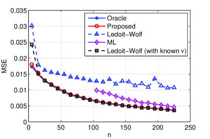
We use (13) with and employ iterations defined by (8) and (9) with . For comparison, we also plot the results of the trace-normalized oracle in (12), the trace-normalized Ledoit-Wolf estimator [Ledoit2004], and the non-regularized solution in (7) (when ). As the Ledoit-Wolf estimator operates on the sample covariance which is sensitive to outliers, we also compare to a trace-normalized version of a clairvoyant Ledoit-Wolf estimator implemented according to the procedure in [Ledoit2004] with known . More specifically, the samples are firstly normalized by the known realizations , yielding truly Gaussian samples; then the sample covariance of the normalized ’s is computed, which is used to estimate the Ledoit-Wolf shrinkage parameters and estimate the covariance via equation (14) in [Ledoit2004]. The MSE are plotted in Fig. 1. It can be observed that the proposed method performs significantly better than the Ledoit-Wolf estimator, and the performance is very close to the ideal oracle estimator using the optimal shrinkage parameter (12). Even the clairvoyant Ledoit-Wolf implemented with known does not outperform the proposed estimator in the small sample size regime. These results demonstrate the robustness of the proposed approach.
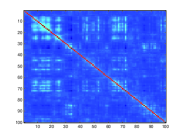
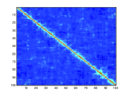
As a graphical illustration, in Fig. 2 we provide covariance visualizations for a realization of the estimated covariances using the Ledoit-Wolf method and the proposed approach. The sample size in this example is set to 50, which is smaller than the dimension 100. Compared to the true covariance, it is clear that the proposed covariance estimator preserves the structure of the true covariance, while in the Ledoit-Wolf covariance procudure produces “block pattern” artifacts caused by heavy-tails of the multivariate Student-T.
When , we also observe a substantial improvement of the proposed method over the ML covariance estimate, which provides further evidence of the power of Steinian shrinkage for reducing MSE.
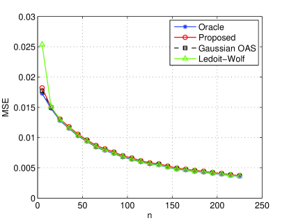
In order to assess the tradeoff between accuracy and robustness we investigate the case when the samples are truly Gaussian distributed. We use the same simulation parameters as in the previous example, the only difference being that the samples are now generated from a Gaussian distribution. The performance comparison is shown in Fig. 3, where four different (trace-normalized) methods are included: the oracle estimator derived from Gaussian assumptions (Gaussian oracle) [Chen], the iterative approximation of the Gaussian oracle (Gaussian OAS) proposed in [Chen], the Ledoit-Wolf estimator and the proposed method. It can be seen that for truly Gaussian samples the proposed method performs very closely to the Gaussian OAS, which is specifically designed for Gaussian distributions. Indeed, for small sample size (), the proposed method performs even better than the Ledoit-Wolf estimator. This indicates that, although the proposed robust method is developed for the entire elliptical family, it actually sacrifices very little performance for the case that the distribution is Gaussian.
V Application to anomaly detection in wireless sensor networks
In this section we demonstrate the proposed robust covariance estimator in a real application: activity detection using a wireless sensor network.
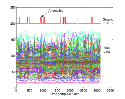
The experiment was set up on an Mica2 sensor network platform, as shown in Fig. 4, which consists of 14 sensor nodes randomly deployed inside and outside a laboratory at the University of Michigan. Wireless sensors communicated with each other asynchronously by broadcasting an RF signal every 0.5 seconds. The received signal strength (RSS), defined as the voltage measured by a receiver’s received signal strength indicator circuit (RSSI), was recorded for each pair of transmitting and receiving nodes. There were pairs of RSSI measurements over a 30 minute period, and samples were acquired every 0.5 sec. During the experiment period, persons walked into and out of the lab at random times, causing anomaly patterns in the RSSI measurements. Finally, for ground truth, a web camera was employed to record the actual activity.

Fig. 5 shows all the received signals and the ground truth indicator extracted from the video. The objective of this experiment was intrusion (anomaly) detection. We emphasize that, with the exception of the results shown in Fig. 10, the ground truth indicator is only used for performance evaluation and the detection algorithms presented here were completely unsupervised.
To remove temperature drifts [AnalogIC] of receivers we detrended the data as follows. Let be the -th sample of the -th RSS signal and denote
| (17) |
The local mean value of is defined by
| (18) |
where the integer determines local window size and is set to 50 in this study. We detrend the data by subtracting this local mean
| (19) |
yielding a detrended sample used in our anomaly detection.
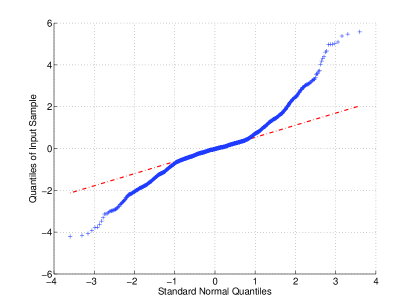
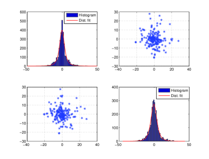
We established that the detrended measurements were heavy-tailed non-Gaussian by performing several statistical tests. First the Lilliefors test [Lilliefors] of Gaussianity was performed on the detrended RSS measurements. This resulted in rejection of the Gaussian hypothesis at a level of significance of . As visual evidence, we show the quantile-quantile plot (QQ plot) for one of the detrended RSS sequences in Fig. 6 which illustrates that the samples are non-Gaussian. In Fig. 7, we plot the histograms and scatter plots of two of the detrended RSS sequences, which shows the heavy-tail nature of the sample distribution. This strongly suggests that the RSS samples can be better described by a heavy-tailed elliptical distribution than by a Gaussian distribution. As additional evidence, we fitted a Student-T distribution to the first detrended RSS sequence, and used maximum likelihood to estimate the degree-of-freedom as with a confidence interval (CI) .
Consider the following function of the detrended data:
| (20) |
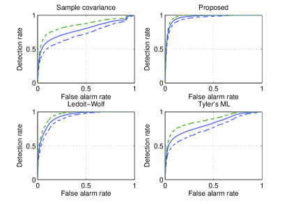
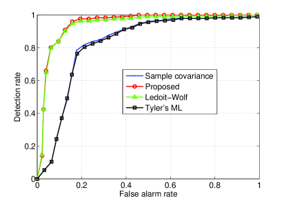
for known , is a statistic that has been previously proposed for anomaly detection [AnomalyDetectionSurvey]. A time sample is declared to be anomalous if the test statistic exceeds a specified threshold. We then applied our proposed robust covariance estimator to estimate the unknown and implemented (20) for activity detection. Specifically, we constructed the sample covariance by randomly subsampling 200 time slices from the RSS data shown in Fig. 5. Note, that these 200 samples correspond to a training set that is contaminated by anomalies at the same anomaly rate (approximately 10%) as the entire sample set. The detection performance was evaluated using the receiver operating characteristic (ROC) curve, where the averaged curves from 200 independent Monte-Carlo trials are shown in Fig. 8. For comparison, we also implemented the activity detector (20) with other covariance estimates including: the sample covariance, the Ledoit-Wolf estimator and Tyler’s ML estimator.
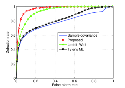
From the mean ROCs we can see that the detection performances are rank ordered as follows: Proposed Ledoit-Wolf Tyler’s ML Sample covariance. The sample covariance performs poorly in this setting due to the small sample size () and its sensitivity to the heavy-tailed distribution shown in Fig. 6 and 7. The Tyler ML method and the Ledoit-Wolf estimator improve upon the sample covariance since they compensate for heavy tails and for small sample size, respectively. Our proposed method compensates for both effects simultaneously and achieves the best detection performance.
We also plot the 90 confidence envelopes, determined by cross-validation, on the ROCs in Fig. 9. The width of the confidence interval reflects the sensitivity of the anomaly detector to variations in the training set. Indeed, the upper and lower endpoints of the confidence interval are the optimistic and the pessimistic predictions of detection performance. The proposed method achieves the smallest width among the four computed confidence envelopes.
Finally, for completeness we provide performance comparison of covariance-based supervised activity detection algorithms in Fig. 10. The training period is selected to be based on ground truth where no anomalies appear. It can be observed that, by excluding the outliers caused by anomalies, the performance of the Ledoit-Wolf based intrusion detection algorithm is close to that of the proposed method. We conclude that the activity detection performance of the proposed covariance estimator is more robust than the other three estimators with respect to outlier contamination in the training samples.
VI Conclusion
In this paper, we proposed a shrinkage covariance estimator which is robust over the class of elliptically distributed samples. The proposed estimator is obtained by fixed point iterations, and we established theoretical guarantees for existence, convergence and uniqueness. The optimal shrinkage coefficient was derived using a minimum mean-squared-error framework and has a closed-form expression in terms of the unknown true covariance. This expression can be well approximated by a simple plug-in estimator. Simulations suggest that the iterative approach converges to a limit which is robust to heavy-tailed multivariate Student-T samples. Furthermore, we show that for the Gaussian case, the proposed estimator performs very closely to previous estimators designed expressly for Gaussian samples.
As a real world application we demonstrated the performance of the proposed estimator in intrusion detection using a wireless sensor network. Implementation of a standard covariance-based detection algorithm using our robust covariance estimator achieved superior performances as compared to conventional covariance estimators.
The basis of the proposed method is the ML estimator originally proposed by Tyler in [Tyler87]. However, the approach presented in this paper can be extended to other M-estimators.
One of the main contributions of our work is the proof of uniqueness and convergence of the estimator. This proof extends the results of [Tyler87, Pascal] to the regularized case. Recently, an alternative proof to the non-regularized case using convexity on manifolds was presented in [Auderset]. This latter proof highlights the geometrical structure of the problem and gives additional insight. We are currently investigating its extension to the regularized case.
VII Acknowledgement
The authors would like to thank Neal Patwari for designing the intrusion detection experiment and collecting the data. We also thank Harry Schmidt and his group at Raytheon, Tucson AZ, for lending us the Mica2 motes for this experiment. We would like to thank Prof. Drton for fruitful discussions and a preprint of [Drton].
VIII Appendix
VIII-A Proof of Theorem 1
In this appendix we prove Theorem 1. The original convergence proof for the non-regularized case in [Tyler87, Pascal] is based on careful exploitation of the specific form of (6). In contrast, our proof for the regularized case is based on a direct connection from the concave Perron-Frobenius theory [Krause94, Krause01] that is simpler and easier to generalize. We begin by summarizing the required concave Perron-Frobenius result in the following lemma.
Lemma 1 ([Krause94]).
Let be a Banach space with being a closed, convex cone on which is increasing, i.e., for which implies , where the operator on the convex cone means that if then . Define . Let be a concave operator such that
| (21) | ||||
If for some and constants , there is
| (22) |
then there exists a unique to which the iteration of the normalized operator converges:
| (23) |
Lemma 1 can be obtained by combining results from Lemma 2 and Theorem in Section 4 of [Krause94]. Here we show that the proof of Theorem 1 is a direct result of applying Lemma 1 with proper definitions of , , and :
-
•
: the set of all symmetric matrices;
-
•
: the set of all positive semi-definite matrices;
-
•
: the normalized nuclear norm of , i.e.,
(24) where is the -th eigenvalue of and is the absolute value operator. Note that for any , the nuclear norm is identical to and is increasing;
-
•
: the set ;
-
•
: the mapping from to defined by
(25) where the weight function is defined as
(26) for any .
Proof:
With the above definitions we show that Theorem 1 is a direct result of Lemma 1. We begin by showing that the mapping operator is concave. Indeed, it is sufficient to show that in concave in , which is true because it is the infinimum of affine functions of .
Next, we show that satisfies condition (22) with . It is easy to see that
| (27) |
for any . Then we show that
| (28) |
for any . Indeed,
| (29) |
where is the maximum eigenvalue of . The last equality in the right-hand-side of (29) comes from the fact that is of unit norm by definition (4). (28) is thus obtained by noticing that and . Substituting (28) into (25) we have
| (30) |
where
and is the maximum eigenvalue of . Again, as is of unit norm, and
| (31) |
Therefore, we have shown that satisfies condition (22), where , and . In addition, (22) establishes that the mapping from always yields a positive definite matrix. Therefore, the convergent limit of the fixed-point iteration is positive definite.