Thermodynamic and dynamic anomalies in a one dimensional
lattice model of liquid water
Abstract
We investigate the occurrence of waterlike thermodynamic and dynamic anomalous behavior in a one dimensional lattice gas model. The system thermodynamics is obtained using the transfer matrix technique and anomalies on density and thermodynamic response functions are found. When the hydrogen bond (molecules separated by holes) is more attractive than the van der Waals interaction (molecules in contact) a transition between two fluid structures is found at null temperature and high pressure. This transition is analogous to a ‘critical point’ and intimately connects the anomalies in density and in thermodynamic response functions. Monte Carlo simulations were performed in the neighbourhood of this transition and used to calculate the self diffusion constant, which increases with density as in liquid water.
pacs:
61.20.Gy,65.20.+wI Introduction
Liquid water has many properties which are recognized as being anomalous when compared to other nonbonded liquids with the same molecular size. As an example, the isothermal compressibility and the constant pressure heat capacity present minimum as a function of temperature at ambient pressure. In addition, the thermal expansion coefficient is negative below , indicating that density increases anomalously with temperature debenedetti04:review ; Franks:water:matrix . Besides thermodynamic anomalies, water present dynamic anomalies. For temperatures below there is a region where the self-diffusion constant increases as a function of pressure debenedetti04:review ; marcia:jcp .
The thermodynamic anomalies seems to be inter-related and different thermodynamic scenarios were proposed to describe these relations debenedetti04:review . Here we will focus our discussion on the second critical point scenario poole92:nat , that is supported by the model studied here (as will be shown latter). According to this scenario, the diverging thermodynamic behavior of the response functions is associated with the critical point arising from metastable liquid-liquid phase transition that occurs in the supercooled regime, in an experimentally unaccessible temperature below the homogeneous nucleation temperature. This scenario was originally observed and proposed by means of computer simulations of atomistic models for liquid water poole92:nat , but there are indirect experimental evidences for the existence of a liquid-liquid phase transition in supercooled water on amorphousmishima98:nat1 ; mishima98:nat2 and confined waterchen08:epj .
The relation between thermodynamic and dynamic anomalies have been subject of discussion in the literature debenedetti01:nat ; chen08:epj ; Truskett07:jcp1 ; truskett07:jpcb . Using atomistic models of water, Errington and Debenedetti found that the anomalously diffusive region surrounds the region of density anomaly in the temperature vs. density plane debenedetti01:nat . In addition, measures of translational and rotational structure also reveals unexpected behavior, that could be connected to the anomalies on density and diffusion debenedetti01:nat . These relations, usually called hierarchy of anomalies, are not restricted to water models and where observed in computer simulations of sharma06:jcp ; charusita09:prer , charusita09:prer , and core-softened models of fluids marcia08:jcp ; truskett06:jcp1 ; truskett07:jpcb .
With the aim of investigating the relation between thermodynamic and dynamic anomalies of water we propose a one dimensional lattice model of water. Lattice and off-lattice one dimensional models of water were proposed by Ben-Naimben-naim08:jcp ; ben-naim08:jcp2 ; Ben-Naim:statmech , Bellbell69:jmath , and others robinson96:prl ; stanley99:pre , to investigate the so-called thermodynamic anomalies and even the unusual solvation behavior presented by water. Nevertheless, and as far as we know, the behavior of the equilibrium diffusion constant of these models were not investigated.
The thermodynamics of our model is obtained exactly using transfer matrix technique and its dynamics is investigated through Monte Carlo simulations. A waterlike anomalous behavior is found both on density and self diffusion constant, as observed in water debenedetti04:review and atomistic models of water marcia:jcp ; stanley07:pre:yan .
This paper is organized as follows. In section II we build the model’s Hamiltonian and investigate its ground state. In section III the thermodynamics of the model is analysed and discussed. Monte Carlo simulations are used to calculate the self-diffusion constant on section IV and the relation between thermodynamics and kynetics is explored on section IV.1. Final remarks are made on the last section.
II The model
The model consists of a linear lattice whose sites can be either occupied by molecules or empty. Two interactions are defined: a short-range van der Waals attraction between nearest neighbours and a hydrogen bond between second nearest neighbours separated by holes. An occupation variable is assigned to each site to indicate the presence () or the absence ( of a molecule. With these definitions the effective Hamiltonian in the grand canonical ensemble is written as:
| (1) | |||||
where defines the strength of the van der Waals attraction, the strength of the hydrogen bond, and is the chemical potential.
In order to obtain a preliminary insight about the model we investigate the ground state by looking at three states putative states at null temperature: a gas (G), a bonded fluid (BF) and a dense fluid (DF). The gas phase is an empty lattice which ‘coexists’ with the fluid phase of lower free energy at null pressure. The bonded fluid is a half filled and fully bonded lattice, while the dense fluid is a filled lattice without bonds. For a lattice with size and periodic boundary conditions, the grand canonical free energies of the fluid phases are and . We will only consider parameters that correspond to the hydrogen bond being more attractive than the van der Waals interaction, i.e., , in consistence with real water. In fact, this condition also ensures the predominance of a bonded fluid at low temperatures and pressures in the range , with . At null temperature, a transition between the BF and the DF happens at , as observed by Sadr-Lahijany et al. in a similar continous model stanley99:pre . Here we follow ref. stanley99:pre on calling this null temperature transition as the ‘second critical point’, in addition to the ‘critical point’ found at and . Further discussions about the ‘second critical point’ of this system will be made on section III.1.
III Thermodynamics

We use the transfer matrix technique to exactly calculate the grand canonical partition function (more details can be found on appendix A) of Hamiltonian (1) as
| (2) |
where , , and are, respectively, the thermodynamic variables temperature, system’s length, chemical potential and pressure, and , with the Boltzmann constant. From the density becomes:
| (3) |
where and . It is shown on appendix A that the density can be written in terms of these quantities as:
In addition to the density , the densities (per site) of hydrogen bonds () and nearest neighbours () are also important to relate the liquid structure to the anomalous behavior and are calculated on appendix A. The mean number of hydrogen bonds () and nearest neighbours () per particle can be calculated from those expressions as and .
The thermodynamic response functions are important to characterize waterlike behavior, particularly because they indicate the possibility of a critical behavior on the supercooled regime (as is expected to occur in liquid water). Here we investigate the thermal expansion coefficient () and isothermal compressibility (), defined as:
| (4a) | |||||
| (4b) | |||||
Expressions for these functions are lengthy and they will not be presented here.
III.1 Low temperature limit
Let us note that for expression (3) results in a null density . Nevertheless, at null temperature the limiting value of the density depends on how the point (,) is approached, due the ‘transition’ occuring at this point. While approached from above, the density is compatible with the BF ground state (see the second column of Tab. 1). In addition, both and diverges while approaching this ‘critical point’ (not shown). An equivalent behavior was previously obtained by Sadr-Lahijany et al. in a similar continous model stanley99:pre . Even more interesting is the low-temperature behaviour of the system in the neighbourhood of the second critical point (,). In what follows we analyse this behavior focusing on density and its derivative . From now on we assume . Using this one obtains the low temperature limit of eq. (3) as
| (5) |
where it was assumed that at small temperatures. By applying this expression to the point it follows that while the point is approached from above, as discussed before.
Now, we note that in the neighbourhood of the fluid-fluid transition at
and define
in order to simplify eq. (5). While approaching this transition it can be found that for , for and when . Using these definitions, eq. (5) is written as
| (6) |
The low-temperature limits of the density and the derivatives of (6) are obtained in a straightforward manner (see Tab. 1). It is particularly interesting to note that the values expected from section II are reobtained when the ‘critical’ pressure is approached from below or from above, see table 1. Nevertheless, when null temperature limit is approached with one finds , which is different from both BF and DF. This is an indication of a new liquid structure, which can be represented through a serie of two neighbouring water molecules surrounded by empty sites. By comparing the expected grand canonical free energies, it was verified a posteriori that this state coexists with both BF and DF exactly at . The existence of such a hidden state make the analysis of the ground state limit more complex. Nevertheless, a simple derivation similar to the one presented above, was used for obtaining the low-temperature limiting values of the densities of hydrogen bonds (17) and nearest neighbours (18) presented on table 1.
We finish this analysis noting that the behavior of the thermal expansion coefficient in the neighbourhood of the fluid-fluid phase transition changes qualitatively depending on how the ‘second critical point’ is approached. For a linear approach we find , which is reasonable since the density anomalous increase with temperature in region dominated by BF fluid structure, for or equivalently .
III.2 Liquid structure
In what follows we analyse the thermodynamic liquid structure in the pressure vs. temperature phase diagram for the parameter . Similar features are found for other parameter values, provided that .
Fig. 1 shows that the line of temperature of maximum density (TMD) starts at exactly at the BF-DF transition, which has the peculiar property that
This line reaches its maximum temperature at and then its temperature decreases with pressure until reaching the G-BF transition located at . As discussed previously by Sadr-Lahijany et al. stanley99:pre , the G-BF transition is a remanent of a gas-liquid phase transition of a system with higher dimensionality, and can be found in simple 1D fluids with attractive short-range interactions. The very fact that the TMD connects two transitions (G-BF and BF-DF) seems to be a peculiar property of some 1D models, since a similar feature also occurs in the 1D lattice model proposed by Bell bell69:jmath and for some parameters in reference stanley99:pre , but not int the continuous models studied in bell69:jmath ; ben-naim08:jcp .
a 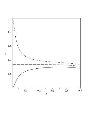 b
b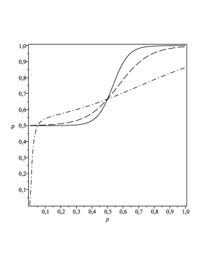
c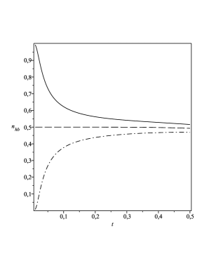 d
d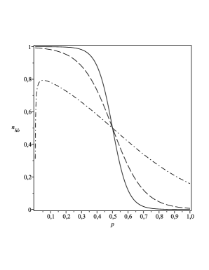
e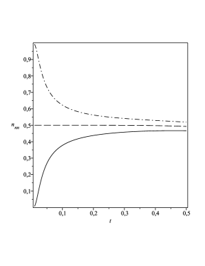 f
f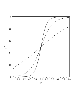
In Fig. 2 the behavior of density, number of hydrogen bonds and number of nearest neighbours per particle is compared as a function of temperature and pressure. Figs. 2 (a), (c) and (e) show that the anomalous increase in density with temperature (for ) is followed by a decrease on the number of hydrogen bonds and by an increase on the number of first nearest neighbours. For , not only is persistent for a wide range of temperatures, but is also found in the same region. Figs. 2(b), (d) and (f) show that the continuos transition between BF and DF progressively becomes more abrupt as the temperature is lowered. From these figures, it is also evident that , and are essentialy not changing with temperature at , since different isotherms cross at this point. These results indicate that the intermediate fluid structure discussed in the previous section is well populated in a borderline separating a BF-like region from a DF-like region. It is possible that this population occurs because the intermediate structure is an unavoidable intermediate step for changing between the BF and DF liquid structures. A last comment about Figs. 2 (b), (d) and (f) is approapriate at this point: it is evident from the high temperature curves that a fast transition between the G and BF structures takes place at low pressures. This is associated with the low- and low- part of the TMD, which happens with a fast but small increase in density with temperature, as also observed in Figs. 5 and 6 from reference bell69:jmath .
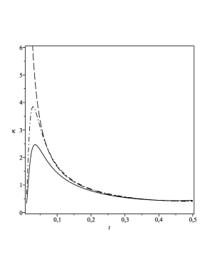
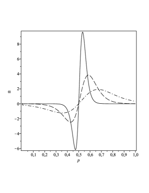
The isothermal compressibility is presented in Fig. 3 as a function of temperature, at the same pressures as Figs. 2(a), (c) and (e). Note that increases with decreasing temperature in the neighbourhood of of the BF-DF transition, and that it diverges when approaching this transition with . The diverging behavior of can be more easily understood as a function of pressure with fixed temperature, as in Fig. 4. Note that, while approaching the BF-DF transition through a pressure decrease, is diverging to in the BF side and to on the DF side, as discussed in the previous section.
In the next section we turn our attention to Monte Carlo simulations used to study the anomalous behavior of the diffusion constant of this model.
IV Monte Carlo Simulations

Monte Carlo simulations were performed in the canonical ensemble using jumps to nearest and next-nearest neighbour sites. Next-nearest neighbour jumps are necessary to observe diffusion in one dimensional lattice fluids since it is impossible for the particles to turn around their neighbours 111Without next nearest neighbour jumps this model presents a more complex subdiffusive dynamics..
Each simulation starts with particles placed randomly along sites of a linear lattice with periodic boundary contourn, at temperature . The initial configuration is recorded in a vector with the position of each molecule. On each MC timestep particles are randomly selected to jump and, in the absence of a collision, the Metropolis algorithm is applied to test the acceptance of the movement binder . After an equilibration time the mean square displacements in relation to the initial configuration is calculated and recorded at every timesteps until the simulation time . A number of different simulations is performed to avoid dependences on initial conditions. The diffusion constant is then obtained by interpolating the Einstein equation:
| (7) |
where the average is performed over the initial conditions.

This protocol was used to simulate a system of size , with the temperature ranging from to and the density in the interval . The simulation times used for this system was , and ; and a number of different initial configurations were performed on each point. The error on the diffusion constant was smaller than in all cases.
IV.1 Anomalous Diffusion and Hierarchy of anomalies
The self-diffusion is shown in Fig. 5 as a function of density for five different temperatures. At high temperatures, and particularly for in Fig. 5, the diffusion decreases with density, as expected in a system with simple hard core particles. For temperatures below it is possible to observe points of minimum () and maximum () diffusion, as a function of density. Between and the self-diffusion constant anomalously increase with density, as happens for water in a region of the phase diagram debenedetti04:review . The presence of a minimum in diffusion was observed in atomistic debenedetti01:nat models of liquid water, as well as continuous marcia08:jcp ; barraz09:jcp and lattice marcia07:pa ; marcia07:pa2 ; szortyka10:jcp models with waterlike behavior but, as far as we know, this is the first time that this behavior is observed in a one dimensional lattice model.
In order to locate and points on the neighbourhood of minimum and maximum diffusion were fitted with the function:
| (8) |
with , , , , , , and as numerically adjustable parameters. At low temperatures (), two parameter sets were used to fit , with at least points around each extrem. For temperatures higher than a single function was used to fit at least points covering both extrems. Maximum and minimum values of diffusion were calculated through the derivative of eq. (8). Points of extremum diffusion are compared to the exact TMD line in the density vs. temperature phase diagram on Fig. 6. Even though not reaching the typically lower temperatures of the region anomalous in density, the simulations indicate that for less dense states () the line of minimum diffusion occurs at temperatures higher than the TMD line. For higher densities, the line of maximum diffusion presents a reentrance and it crosses the TMD line, indicating that an strict hierarchy of anomalies is absent on this simplified model (at least for ).
By comparing Fig. 6 and similar results from other lattice models marcia07:pa ; marcia07:pa2 ; szortyka10:jcp one observes an overall tendency of overlap between regions of anomalous diffusion and density. Nevertheless, the so-called hierarchy of anomalies does not always occur in simple hierarchical structure, as found in atomistic models of water debenedetti01:nat ; stanley07:pre:yan . In two-dimensional lattice models with waterlike behavior a hierarchy of anomalies was found in a reversed order, i.e., with the TMD line covering the anomalously diffusive region marcia07:pa2 ; szortyka10:jcp . On the other side, a three dimensional lattice model also presents a line of extremum diffusion crossing the TMD, as in this work, but with the region of diffusion anomaly covering the TMD at low densities marcia07:pa . Considering these models and the results presented on this paper it is possible to conclude that there is an overall tendency for the concomitant ocurrence of density and diffusion anomalies but the existence of an hierarchical order between these anomalies depends on dimentionality and even on possibily on the detailed nature of the interactions between molecules.
V Conclusion
We introduced a simple one dimentional lattice-gas model that reproduces waterlike anomalies on its thermodynamics and dynamics through transfer matrix technique and Monte Carlo simulations. Although other models were used to investigate water’s peculiar propertiesbell69:jmath ; ben-naim08:jcp ; stanley99:pre ; robinson96:prl , (as far as we know) this is the first time this type of model is used to investigate the inter-relations between thermodynamic and dynamic waterlike anomalies.
Our results show that the region of thermodynamic anomalies is located in the neighbourhood of the transition between two structured fluids: a bonded fluid (BF) and a dense fluid (DF). The null temperature ‘second critical point’ is linked to this transition and the relation between the criticality and the temperature of maximum density can be understood from the behavior of the thermal expansion coefficient in the vicinity of the critical point.
An increase on the diffusion coefficient with density (at fixed temperature) was also found in the neighbourhood of BF-DF transition. Even though existing an overall tendency for the concomitant ocurrence of the regions of anomalous diffusion and density, a strict hierarchy of anomalies is absent on this model.
As final remark we mention that the simplicity of the current model makes it an ideal prototype for more detailed investigations on the inter-relations between waterlike thermodynamic and dynamic anomalies. We are now working on analytical approaches to the diffusion constant of this model using techniques from non-equilibrium statistical mechanical. Another approach that is currently under investigation involves the calculation of the diffusion constant through the Kubo relation to understand the connection between memory and diffusion in more complex topologies morgado02:prl .
Acknowledgements
We acknowledge B. Widom for usefull discussions and C. E. Fiore dos Santos for carefully reading the original manuscript of this paper. This work has been supported by the CNPq, FAPDF and FINATEC. MAAB acknowledges finantial support from the National Science Foundation via grant CHE-0842022 during part of this work.
Appendix A Transfer matrix technique
Here we use the transfer matrix technique to calculate the grand canonical partition function of linear chain with Hamiltonian (1). More detailed survey of the technique can be found on textbooks of statistical mechanical salinas:introduction ; Ben-Naim:statmech . Since our model does present interactions up to three neighbouring lattice sites, we will rewrite the Hamiltonian as
| (9) |
where periodic boundary conditions are assumed implicitly. The three-site interaction Hamiltonian is defined as
| (10) | |||||
A simple procedure to represent the transfer matrix of in a one dimensional system with first and second nearest neighbour interactions is described by Ben-Naim Ben-Naim:statmech . Following this procedure, the grand canonical partition function can be written as
| (11) |
where the sum is made over all lattice states and . Let us now define an auxiliar occupation variable and a new Boltzmann weight as
| (12) |
It is not difficult to use to write (11) as trace of a matrix:
| (13) |
where the elements of matrix are ordered through binary numbers whose bits are occupation variables, and are given by:
In the thermodynamic limit, only the largest eigenvalue () of contributes to the right hand side of eq. (13), and this equation becomes
| (14) |
where the characteristic polynomial of is
| (15) |
By solving together equations (14) and (15) one can obtain either or . Here we follow Bell in ref. bell69:jmath , who noted that can be rearranged from (15) as a function of , and ; leaving the possibility of calculating the density as
| (16) | |||||
Finally, the same procedure can be used to calculate the densities of hydrogen bonds and nearest neighbours (per site) as
| (17) | |||||
| (18) |
References
- (1) P. G. Debenedetti, J. Phys.: Cond. Matter 15, 1669 (2003)
- (2) F. Franks, Water: a Matrix for life (second edition) (Royal Society of Chemistry, 2000)
- (3) P. A. Netz, F. W. Starr, H. E. Stanley, and M. C. Barbosa, J. Chem. Phys. 115, 344
- (4) P. H. Poole, F. Sciortino, U. Essmann, and H. E. Stanley, Nature 360, 324 (1992)
- (5) O. Mishima and H. E. Stanley, Nature 396, 329 (1998)
- (6) O. Mishima and H. E. Stanley, Nature 392, 164 (1998)
- (7) F. Mallamace, C. Branca, M. Broccio, C. Corsaro, N. Gonzalez-Segredo, J. Spooren, H. E. Stanley, and S.-H. Chen, Eur. Phys. J. Special Topics 161, 19 (2008)
- (8) J. R. Errington and P. G. Debenedetti, Nature 409, 318 (2001)
- (9) J. R. Errington, T. M. Truskett, and J. Mittal, J. Chem. Phys. 127, 244502 (2007)
- (10) J. Mittal, J. R. Errington, and T. M. Truskett, J. Phys. Chem. B 111, 10054 (2007)
- (11) R. Sharma, S. N. Chakraborty, and C. Chakravarty, J. Chem. Phys. 125, 204501 (2006)
- (12) M. Agarwal and C. Chakravarty, Phys. Rev. E 79 (2009)
- (13) A. B. Oliveira, G. Franzese, P. A. Netz, and M. C. Barbosa, J. Chem. Phys. 128, 064901 (2008)
- (14) J. Mittal, J. R. Errington, and T. M. Truskett, J. Chem. Phys. 125 (2006)
- (15) A. Ben-Naim, J. Chem. Phys. 128, 024505 (2008)
- (16) A. Ben-Naim, J. Chem. Phys. 128 (2008)
- (17) A. Ben-Naim, Statistical Mechanics for Chemists and Biochemists (Plenum, New York, 1992)
- (18) G. M. Bell, J. Math. Phys. 10, 1753 (1969)
- (19) C. H. Cho, S. Singh, and G. W. Robinson, Phys. Rev. Lett. 76, 1651 (1996)
- (20) M. R. Sadr-Lahijany, A. Scala, S. V. Buldyrev, and H. E. Stanley, Phys. Rev. E 60, 6714 (1999)
- (21) Z. Yan, S. V. Buldyrev, P. Kumar, N. Giovambattista, P. G. Debenedetti, and H. E. Stanley, Phys. Rev. E 76, 051201 (Nov 2007)
- (22) Without next nearest neighbour jumps this model presents a more complex subdiffusive dynamics.
- (23) K. Binder and D. W. Heermann, Monte Carlo simulation in statistical physics (Springer-Verlag, 1988)
- (24) J. N. M. Barraz, E. Salcedo, and M. C. Barbosa, J. Chem. Phys. 131, 094504 (2009)
- (25) M. Girardi, M. Szortyka, and M. C. Barbosa, Physica A 386, 692 (2007)
- (26) M. Szortyka and M. C. Barbosa, Physica A 380, 27 (2007)
- (27) M. M. Szortyka, C. E. Fiore, V. B. Henriques, and M. C. Barbosa, J. Chem. Phys. 133 (2010)
- (28) R. Morgado, F. A. Oliveira, G. G. Batrouni, and A. Hansen, Phys. Rev. Lett. 89, 100601 (Aug 2002)
- (29) S. R. A. Salinas, Introduction to statistical physics (Springer-Verlag, New York, 2001) Chap. 13.