Testing the statistical isotropy of large scale structure with multipole vectors

Abstract

A fundamental assumption in cosmology is that of statistical isotropy — that the universe, on average, looks the same in every direction in the sky. Statistical isotropy has recently been tested stringently using Cosmic Microwave Background (CMB) data, leading to intriguing results on large angular scales. Here we apply some of the same techniques used in the CMB to the distribution of galaxies on the sky. Using the multipole vector approach, where each multipole in the harmonic decomposition of galaxy density field is described by unit vectors and an amplitude, we lay out the basic formalism of how to reconstruct the multipole vectors and their statistics out of galaxy survey catalogs. We apply the algorithm to synthetic galaxy maps, and study the sensitivity of the multipole vector reconstruction accuracy to the density, depth, sky coverage, and pixelization of galaxy catalog maps.

I Introduction

In the standard model of cosmology the primordial density perturbations in the early Universe are generated by a Gaussian, statistically isotropic random process. There are two reasons for this: the cosmological principle tells us that the Universe is homogeneous and isotropic on large scales and the standard (single-field, slow-roll) inflationary theory predicts near-perfect Gaussianity and statistical isotropy of primordial fluctuations in the universe.

It is useful to differentiate the sometimes conflated concepts of statistical isotropy (hereafter SI) and Gaussianity. Statistical isotropy means that the expectation values of measurable quantities are invariant under rotations. For example, the expected two-point correlation function of the Cosmic Microwave Background (CMB) temperature (or galaxy overdensity) $\Delta$ in two directions in the sky $\hat{e}_{i}$ and $\hat{e}_{j}$

$$C(\hat{e}_{i},\hat{e}_{j})=\langle\Delta(\hat{e}_{i})\Delta(\hat{e}_{j})\rangle$$ (1)

(where $\langle\cdot\rangle$ represents the ensemble average) would, under SI, depend only on the angle $\theta$ between $\hat{e}_{i}$ and $\hat{e}_{j}$, i.e. $C(\hat{e}_{i},\hat{e}_{j})=C(\hat{e}_{i}\cdot\hat{e}_{j})$. Gaussianity, on the other hand, refers to the statistical distribution from which the quantity $\Delta$ is drawn. As a consequence of Gaussianity, all of the statistical properties of the field are encapsulated in the two-point correlation function $C(\hat{e}_{i}\cdot\hat{e}_{j})$; all of the odd higher-point correlation functions are zero, and the even-point correlation functions can be related to the two-point function by Wick’s theorem. In general, a given field can be Gaussian but not SI, or SI but not Gaussian, or neither. The standard cosmological theory predicts it to be both (except to the extent that nonlinear evolution spoils the Gaussianity).

Much of the information used to construct the current concordance model has been derived from examination of the statistical properties of the CMB temperature anisotropies on the sky. Following in the footsteps of the Cosmic Background Explorer (COBE) COBE ; COBE2 , experiments such as the Wilkinson Microwave Anisotropy Probe (WMAP) Spergel2003 ; Spergel2006 ; wmap7 have succeeded in measuring the temperature anisotropies to high precision, engendering widespread confidence that we have arrived at a convincing model, based on standard inflationary cosmology, in which the perturbations are presumably Gaussian and statistically isotropic.

However, certain anomalies at low $\ell$ have been pointed out and suggest possible deviations from this paradigm. Over a decade ago, the COBE Differential Microwave Radiometer (COBE-DMR) first reported a lack of large-angle correlations in the two-point angular-correlation function, $\mathcal{C}(\theta)$, of the CMB DMR4 . This was confirmed by the WMAP team in their analysis of their first year of data Spergel2003 , and by some of us in the WMAP three, five and seven-year data wmap123 ; wmap12345 ; Sarkar , and further confirmed by independent analyses Hajian:2007pi ; Bunn_Bourdon . The angular two-point function is approximately zero at scales $\theta>60^{\circ}$ in all wavebands, in contrast to the theoretical prediction from the standard inflationary cosmology. Such a result is expected in only $\sim 0.03$% of the Gaussian random, isotropic skies based on the standard inflationary model (and using a statistic suggested in Spergel2003 ). This vanishing of $C(\theta)$ is unexpected not only because of its low likelihood (which admittedly has been defined a posteriori), but for at least four other reasons. First, missing correlations are inferred from cut-sky (i.e. masked) maps of the CMB, which makes the results insensitive to assumptions about what lies behind the cut. Second, what little large-angle correlation does appear in the full-sky maps is associated with points inside the masked region, further casting into doubt the full-sky reconstruction-based results (wmap12345, ). Third, the vanishing power is not as clearly seen in multipole space where the quadrupole is only moderately low, and it is really a range of low multipoles that conspire to “interfere” in just such a way to make up the near-vanishing $C(\theta)$ (wmap12345, ). Fourth, the missing power occurs on the largest observable scales, where a cosmological origin is arguably most likely.

Moreover, some of us and others found that the two largest cosmologically interesting modes of the CMB, the quadrupole and octopole ($\ell=2$ and $3$), are correlated with the direction of motion and geometry of the solar system (Schwarz2004, ). [Recall that each multipole $\ell$ corresponds to scales of about $180/\ell$ degrees on the sky]. In brief, the quadrupole and octopole are unusually planar (as first pointed out by TOH ); their plane is perpendicular to the ecliptic plane and pointed to the cosmic dipole; and the ecliptic plane itself traces out a nodal line between the big hot and cold spots in the quadrupole-octopole map. The alignments persist to smaller scales (higher multipoles of the CMB), where it has been found that $\ell\leq 6$ multipoles have unusually large fraction of power in a preferred frame (Land2005a, ). Even at the first peak, it has been shown (Yoho:2010pb, ) that there is an ecliptically-associated anomaly – the first peak is significantly under-powered near the north ecliptic pole. It has also been found that the northern ecliptic hemisphere has significantly less power than the southern hemisphere on scales larger than about 3 degrees (multipoles $\ell\lesssim 60$) (Eriksen_asym, ; Hansen_asym, ; Eriksen:2007pc, ; Hansen:2008ym, ; Hoftuft, ). These non-Gaussianities at large and small scales have been confirmed by other analyses (Raeth:2010kx, ). These alignments, being indicative of a real effect whether it is cosmological or astrophysical, have caused wide interest, and some of us followed them up by performing a comprehensive study of the findings and comparing different statistics, considering the foreground contamination, and studying the COBE data as well (lowl2, ). The most recent WMAP paper on anomalies Bennett_anomalies , while disagreeing with some of the above findings and agreeing with others, does not appear to offer convincing explanations of the observed anomalies. For a brief review of the anomalies, see Huterer_NewAst_review ; for a comprehensive review, see CHSS_review .

At this time there is no convincing explanation for alignments or the missing large-angle correlations found in the CMB. However, the consequences are clear: if indeed the observed $\ell=2$ and $3$ CMB fluctuations are not cosmological, one must reconsider all cosmological results that rely on low $\ell$ of the CMB. Even more importantly, a cosmological origin of the violation of statistical isotropy would invalidate the basic assumptions used in the standard analyses to extract cosmological parameters, requiring our full understanding of the physics behind the anomalies.

In the past 15 years or so, galaxy surveys have revolutionized our understanding of the universe. Most recently, the Sloan Digital Sky Survey (SDSS) and the Two Degree-Field Survey (2dF) have measured the locations of about a hundred million galaxies over $\sim\!10,000$ sq. deg. of the sky, and measured about a million redshifts. The main product of these massive efforts was precision measurement of the cosmological parameters, and also the precise measurement of the matter power spectrum. Perhaps surprisingly, however, except for a few searches for modulations in power in the large-scale structure (LSS) Hirata ; Pullen_Hirata and theoretical predictions for clustering of halos in models that break the SI Ando:2008zza , there have been few explicit tests of statistical isotropy using the LSS. Instead, most of the studies have been either theoretical or applied exclusively to the CMB, and concerned with how the CMB anisotropy would look in inflationary (or other) models that break SI Gordon2005 ; ACW ; Donoghue:2007ze ; ArmendarizPicon07 ; Gumrukcuoglu ; Rodrigues_Bianchi ; Pullen_Kam ; Pitrou08 ; Erickcek_hem ; Erickcek_iso ; Battye09 . Such models, where the primordial power spectrum $P({\bf k})$ depends on the magnitude and direction $\hat{{\bf k}}$ of the wavevector, may be detectable with WMAP or future CMB experiments, and there has recently been a lot of effort searching for signatures of broken SI in the CMB Gordon2005 ; Groeneboom:2008fz ; Hoftuft ; Hanson_Lewis ; Groeneboom_sys ; Bennett_anomalies ; Hanson_beams . Given that a set of robust statistical tools have been developed for such tests of the CMB, the natural next step would be to adopt some of the same methods to the study of LSS.

The CMB anomalies found using WMAP data have only whetted the appetite of cosmologists to investigate the aforementioned anomalies further. While the Planck CMB mission will — like WMAP — surely produce spectacular results revolutionizing our understanding of the universe, it is generally expected that Planck will confirm WMAP’s findings on the largest scales as both experiments are measuring the same physical phenomenon at scales where Planck’s better resolution makes no difference. Observations of large-scale fluctuations are subject to sample variance (sometimes referred to as cosmic variance): our universe provides only a relatively small number of independent samples of largest-scale structures, limiting the extent to which the CMB alone can shed light on them. Therefore, it is imperative to extract every last bit of information provided. In particular, galaxy surveys complement the CMB in providing a picture of the largest scales with different tracers of fluctuations than the CMB, emitting light at different wavelengths, and whose analysis includes different systematic errors than that of the CMB. Here we propose to stringently test the cosmological principle using archival data from the upcoming large-scale structure surveys.

This is an excellent time to perform analyses of statistical isotropy on the largest observable scales because full-sky maps of the LSS, with tracers at multiple wavelengths, are finally becoming available. In this paper we adapt the statistical tools used in tests of SI of the CMB to LSS measured by galaxy surveys. We investigate how the characteristics of LSS surveys impact the accuracy of the extracted quantities and present one example of the efficacy of detecting alignments in a specific, purely phenomenological, toy model.

The structure of this paper is as follows. In Sec. II, the relevant cosmological quantities are defined and followed, in Sec. III, by a brief overview of the statistical tools available to conduct tests of SI. In Sec. IV we construct a framework in which the LSS observables are mapped to the selected statistics. The reconstruction technique used to estimate these quantities and how the accuracy of the reconstruction varies with the characteristics of the galaxy survey are discussed in Sec. V. We then proceed to test how this accuracy translates into detection of possible violations of SI in Sec. VI. In Sec. VII we discuss our findings and future work.

II Preliminaries

Consider a cosmological dataset which can be characterized by the function $f(\theta,\phi)$ on the celestial sphere. It can be decomposed into multipole moments as follows:

$$f(\theta,\phi)=\sum_{\ell}f_{\ell}(\theta,\phi)=\sum_{\ell=0}^{\ell=\infty}\sum_{m=-\ell}^{\ell}a_{\ell m}Y_{\ell m}\left(\theta,\phi\right),$$ (2)

where $0\leq\theta\leq\pi$ and $0\leq\phi\leq 2\pi$ and the $a_{\ell m}$ are the multipole coefficients and the complex spherical harmonic functions are given by

$$Y_{\ell m}\left(\theta,\phi\right)=\sqrt{\frac{(2\ell+1)(\ell-m)!}{4\pi(\ell+m)!}}P_{\ell m}\left(\cos\theta\right)e^{im\phi},$$ (3)

where $P_{\ell m}$ are the associated Legendre polynomials. If the cosmological data are indeed produced by a statistically isotropic and Gaussian process, then the $a_{\ell m}$ are realizations of Gaussian random variables of zero mean, characterized fully by their variances. The added property of statistical isotropy (SI) further implies that their variances depend only on $\ell$ and means that we can write

$$C_{\ell m\ell^{\prime}m^{\prime}}\equiv\langle a_{\ell m}a^{*}_{\ell^{\prime},m^{\prime}}\rangle=C_{\ell}\delta_{\ell\ell^{\prime}}\delta_{mm^{\prime}}$$ (4)

where $C_{\ell}$ is the expected power in the $\ell$-th multipole. Note that the theoretically predicted coefficients $a_{\ell m}$ and the power spectrum $C_{\ell}$ correspond to averages over an ensemble of universes. While we unfortunately have only a single sample of $a_{\ell m}$ for each $\ell$ and $m$, corresponding to values measured in our universe, the power spectrum $C_{\ell}$ can be estimated with a finite sample variance by averaging the power in $a_{\ell m}$ for each $m$

$$\tilde{{\cal C}}_{\ell}\equiv\frac{1}{2\ell+1}\sum^{\ell}_{m=-\ell}|a_{\ell m}|^{2}.$$ (5)

If SI holds, then $\tilde{{\cal C}}_{\ell}$ is an unbiased estimator of $C_{\ell}$. If Gaussianity additionally holds, then it is the best estimator, with cosmic variance $2\tilde{{\cal C}}^{2}_{\ell}/(2\ell+1)$.

Since the power spectrum can be readily calculated from theory, we can compare predictions of our cosmological models to the observationally determined $C_{\ell}$, placing precise constraints on the parameters.

III Statistical Tools

In this section we consider the various quantities related to the above which can be used to test the isotropic nature of cosmological data which is characterized by the function $f(\theta,\phi)$ on the sky given in Eq. (2).

III.1 Multipole coefficients

A caveat that comes with using the power spectrum as a tool for searches of statistical anisotropies is that it is sensitive to only specific types of departures from SI. It is possible for the distribution of power in $C_{\ell}$ throughout the $m$-modes to violate SI with no bearing on the $C_{\ell}$ spectrum.

It is therefore important to measure quantities that contain information about Gaussianity and SI such as the multipole coefficients $a_{\ell m}$. They are another representation of the information in $f(\hat{\Omega})$, where $\hat{\Omega}=(\theta,\phi)$, related by

$$a_{\ell m}=\int f(\hat{\Omega})Y^{*}_{\ell m}\left(\hat{\Omega}\right)d\Omega.$$ (6)

If $f(\hat{\Omega})$ is a realization of a Gaussian and isotropic process, then the equality in Eq. (4) holds and the $a_{\ell m}$ are independent, random variables with Gaussian distributions and variances that depend only on $\ell$. This implies that the distribution of the overall power throughout the $a_{\ell m}$ (i.e. their magnitudes) should be a function of $\ell$ only and the distribution of the power in a particular scale (i.e. $C_{\ell}$) through the $m$-modes should depend only the selected coordinate system.

In deOliveira2004 , a statistic was introduced which associates an axis with each $\ell$ around which the angular dispersion is maximized

$$S_{\ell}=\text{max}_{{\bf n}}\sum_{m}m^{2}|a_{\ell m}|^{2}.$$ (7)

This statistic finds the frame of reference with its z-axis in the $\hat{{\bf n}}_{\ell}$ direction which maximizes the angular dispersion, with the extent of this preference gauged by the magnitude of _ℓ. As mentioned previously, when applied to the WMAP1 data Spergel2003 , this statistic indicated that $\hat{{\bf n}}_{2}$ and $\hat{{\bf n}}_{3}$ were unexpectedly aligned in a direction in which the power ${\cal C}_{2}$ is significantly suppressed. Another such statistic introduced in Land2005a is

$$r_{\ell}=\text{max}_{m{\bf n}}\left[\frac{{\cal C}_{\ell m}}{\sum_{\tilde{m}}|{a_{\ell\tilde{m}}}|^{2}}\right]$$ (8)

where ${\cal C}_{\ell 0}=|a_{\ell 0}|^{2}$ and ${\cal C}_{\ell m}=2|a_{\ell m}|^{2}$ for $m>0$. Here $r_{\ell}$ is the ratio of power of the $\ell$-th multipole that lies in the $m$ mode in the direction ${\bf n}$. This statistic explicitly returns the axis and direction in which the power distribution is most uneven (i.e. ${\bf n}$) and the extent to which it is uneven (i.e. magnitude of $r_{\ell}$). When applied to the WMAP1 data, this statistic returned the same preferred axis as in deOliveira2004 . These features of the CMB sky may be suggesting inter-$m$ correlations between the $a_{\ell m}$ and a break down of SI.

III.2 Multipole Vectors

While the multipole vector formalism was first introduced by Copi:2003kt into the analysis of the CMB, its full history is much longer. More than 100 years ago, Maxwell Maxwell pointed out that for any real function $f_{\ell}(x,y,z)$, which is an eigenfunction of the Laplacian on the unit sphere with eigenvalue $-\ell(\ell+1)$, there exist $\ell$ unit vectors $\left({\bf v}_{1},{\bf v}_{2},...{\bf v}_{\ell}\right)$ such that

$$f(x,y,z)_{\ell}=\nabla_{{\bf v}_{1}}...\nabla_{{\bf v}_{\ell}}\frac{1}{r}\,,$$ (9)

where $(x,y,z)=(\cos\theta\sin\theta,\sin\theta\sin\phi,\cos\phi)$, $\nabla_{{\bf v}_{\ell}}\equiv{\bf v}_{\ell}\cdot\nabla$ is the directional derivative operator, and $r=\sqrt{x^{2}+y^{2}+z^{2}}$. A multipole can then be represented in terms of $\ell$ unit vectors $\left\{{\bf v}_{\ell,i}\mid i=.1...\ell\right\}$, termed the multipole vectors (MVs) and an invariant scalar $A_{\ell}$. Heuristically, the $\ell$-th multipole of the CMB can be written as a product of $\ell$ unit vectors and an overall normalization so that we can write

$$f_{\ell}\sim A_{\ell}\Pi_{i=1}^{\ell}\left({\bf v}_{\ell,i}\cdot\hat{{\bf e}}\right)$$ (10)

where $\hat{{\bf e}}=\left(\sin\theta\cos\phi,\sin\theta\sin\phi,\cos\theta\right)$ is the unit radial vector. Note that the signs of all the vectors can be absorbed into the sign of $A^{(\ell)}$, so one is free to choose the hemisphere of each vector. These multipole vectors encode all the information about the phase relationships of the $a_{\ell m}$. The MVs can be understood in the context of harmonic polynomials Katz2004 and have many interesting properties (e.g. Dennis2005 ). An efficient algorithm to compute the multipole vectors for low-$\ell$ has been presented in Copi:2003kt and is publicly available MV_code ; other algorithms have been proposed as well Katz2004 ; Weeks04 ; Helling .

Note that multipole vectors are defined in exactly the same way for the galaxy surveys provided one makes the obvious identification

$${\delta T\over T}(\hat{\bf n})\longleftrightarrow{\delta n\over n}(\hat{\bf n})$$ (11)

where $n$ is the number of galaxies (or other tracers of the LSS) per unit area of the sky.

Figure 1 shows the multipole vectors of our sky, with the corresponding multipoles $\ell=2-8$ computed from WMAP’s 3-year Internal Linear Combination (ILC) map Hinshaw:2006ia . Multipole vectors still contain the full information about the map, but are often more sensitive to different aspects of the temperature pattern than the usual spherical harmonic representation.

Figure 1: Multipole vectors of our sky, with the corresponding multipoles $\ell=2-8$ computed from WMAP’s 3-year Internal Linear Combination (ILC) map Hinshaw:2006ia . The lobes represent the CMB temperature pattern seen at each multipole, where the observer is at the center and the observed sky anisotropy can be projected to a sphere of a fixed radius. The sticks are the multipole vectors, each pointing in a fixed direction (or its opposite) on this sphere. Figure kindly provided by Craig Copi.

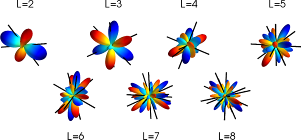
Mutual cross products of $\ell$ vectors in the $\ell$-th multipole define $\ell(\ell-1)/2$ planes, and these planes are also useful for testing the SI. For example, in CHSS_review , the three octopole planes of the CMB were found to be nearly parallel and aligned with the single plane of the quadrupole, and this alignment is statistically significant at the $99.9\%$ level.

To illustrate the advantage of decomposing a multipole in this fashion, we consider MVs of the real part of a pure harmonic mode; $ReY_{\ell m}(\theta,\phi)$, so that all the power $C_{\ell}$ lies in that particular $m$-mode. In this case, $\ell-|m|$ of the $\ell$ MVs are aligned with the $z$-axis (which is the frame of the $Y_{\ell m}$), while the remaining $|m|$ MVs line in the $x-y$ plane. Since the configuration of MVs rotates with the function $f_{\ell}(\theta,\phi)$, the pure harmonic modes are readily identified in any frame of reference. This is true of any function $f_{\ell}(\theta,\phi)$ which makes the MVs very useful for investigation issues such as SI Dennis2004 .

For our purposes the MVs are the quantities of interest and represent all information contained in the data regarding the phase relationships between the $a_{\ell m}$.

IV Large scale structure: mathematical description

Galaxy surveys measure positions of galaxies either in three dimensions (as redshift surveys) or as a 2D projection on the sky (angular surveys). However, most surveys contain information that is somewhere between 2D and 3D, since galaxies have photometric redshifts that enable approximate rendering of radial distance to galaxies (given good knowledge of the underlying cosmological parameters).

In this work we consider projected (i.e. two-dimensional) large-scale structure surveys. We wish to reconstruct the underlying density distribution, $\sigma(\hat{\Omega})$, given counts of galaxies on the sky. When multiplied by the bias parameter $b$, the density field gives an angular number density distribution function of the catalog on the sky $\nu(\hat{\Omega})$.

We can split the number density of objects on the sky, $\nu(\hat{\Omega})$, into its mean and relative variation across the sky

$$\nu(\hat{\Omega})={\bar{\nu}}\left(1+\delta(\hat{\Omega})\right),$$ (12)

where the ${\bar{\nu}}$ is the average density over the sky, given by ${\bar{\nu}}=\int d\Omega~{}\nu(\hat{\Omega})/\int d\Omega$ and $\delta(\hat{\Omega})$ are the fluctuations around the mean at position $\hat{\Omega}$.

To enable connection with observable counts of galaxies, we bin the sky into ${N_{\rm pix}}$ equal-area pixels and define

$$n_{i}=S\int_{{\rm ith~{}pixel}}d\Omega~{}\nu(\hat{\Omega}),$$ (13)

where $n_{i}$ is the expected number of objects in the $i$-th pixel centered at $\Omega_{i}$ and $S$ is a selection function which accounts for the physical attributes of the survey construction, such as the exposure time and the sensitivity of the instruments. For simplicity, we assume that the selection function is independent of direction on the sky; while clearly simplistic, this assumption is straightforwardly relaxed provided that the full selection function is known. Effects of the uncertainties in the selection function, however, may be important and certainly warrant further investigation, but are outside of scope of the present foundational work.

The mean number of expected objects per pixel is then given by

$${\bar{n}}\equiv\frac{1}{{N_{\rm pix}}}\sum_{i=1}^{{N_{\rm pix}}}n_{i}.$$ (14)

We now express the expected fluctuations around the mean $\bar{n}$ by

$$\Delta_{i}\equiv\Delta(\Omega_{i})=\frac{n_{i}-{\bar{n}}}{{\bar{n}}}.$$ (15)

We see that the binned fluctuation $\Delta_{i}$ in the i^th pixel relates to the true underlying fluctuation $\delta$ via

$$\Delta_{i}=\frac{1}{{\Omega_{\rm pix}}}\int_{\rm i^{th}~{}pixel}\delta(\Omega)d\Omega,$$ (16)

where ${\Omega_{\rm pix}}$ is the area of a pixel, so that the $\Delta_{i}$ is the average fluctuation around the mean in the i^th pixel. Hence the disparity between $\Delta_{i}$ at a point $\Omega_{i}$ on the sky and the true underlying $\delta(\Omega_{i})$ depends on the level of pixelization of the sky, so that $\Delta_{i}\to\delta(\Omega_{i})$ in the limit of perfect resolution (${N_{\rm pix}}\to\infty$).

The function $\Delta(\Omega)$ has a constant value $\Delta_{i}$ within the i^th pixel, but otherwise varies across the sky. We expand it into spherical harmonics

$$\Delta(\hat{\Omega})=\sum_{\ell=1}^{\infty}\sum_{m=-\ell}^{\ell}a_{\ell m}Y_{\ell m}(\hat{\Omega})$$ (17)

or

$$\Delta_{i}=\sum_{\ell=1}^{\infty}\sum_{m=-\ell}^{\ell}a_{\ell m}Y_{\ell m}(\Omega_{i}).$$ (18)

We are now able to apply the same treatment of the CMB temperature anisotropies to the case of LSS.

V Multipole Vector reconstruction

V.1 The Reconstruction Methodology

In the last section, we described the transformation of a galaxy catalog into a set of measurements $\Delta\left(\Omega_{i}\right)$ of object numbers in a set of pixels, centered at $\Omega_{i}$ where $i=1...{N_{\rm pix}}$ on the full celestial sphere. The $a_{\ell m}$ can be determined from these observations by inverting Eq. (18)

$$a_{\ell m}=\int Y^{*}_{\ell m}(\hat{\Omega})\Delta(\hat{\Omega})d\Omega={\Omega_{\rm pix}}\sum_{\hat{\Omega}}Y^{*}_{\ell m}(\hat{\Omega})\Delta(\hat{\Omega}),$$ (19)

where $\hat{\Omega}$ is the direction on the sky.

Starting map                                                         Starting map
                      
From cut-sky $a_{\ell m}$                                                      From cut-sky $a_{\ell m}$
                      
Full-sky reconstruction                                             Full-sky reconstruction

Figure 2: Illustration of the efficacy of our reconstruction scheme for a mock galaxy survey with $N_{g}=10^{6}$. The top panel shows our starting map. The middle panels show the map made up from the cut-sky coefficients (i.e. using Eq. 19), while the bottom row shows the full-sky reconstruction that we adopted. The left columns show the full-sky case, while the right columns show the case where $\pm 4.5^{\circ}$ galactic cut (removing $\simeq 8\%$ of pixels) have been applied.

Depending on which tracer objects we are considering for our tests, a fraction of the sky in the direction of the Galactic center may be obscured by stars and dust, as well as point sources. These contaminated regions must typically be avoided in all cosmological analyses of the large-scale structure, just like for the case of the CMB. In the CMB, for example, cosmological signal from the contaminated regions can be recovered using multiwavelength information Bennett_foregr ; LILC , though such cleaning may be risky and prone to biases Tegmark:1995pn ; Hansen:2006rj . For the case of LSS, data is given by the object positions given in (e.g. galaxy) catalogs; thus inevitably we are forced to deal with data that sample only parts of the sky.

The presence of the sky mask and measurement noise imply that Eq. (19) may be inaccurate in reconstructing the $a_{\ell m}$. Instead, one can implement a weighting scheme on the unmasked part of the sky. Such an approach was advocated in deOliveiraCosta:2006zj and applied to the CMB and has been shown to optimally estimate the low-$\ell$ multipoles for cut skies (under certain assumptions about the statistical properties of the sky). We now review this method and apply the reconstruction technique to galaxy catalogs.

Let $x_{i}=\Delta_{i}$ represent the number of objects measured in a pixel centered at the points $\Omega_{i}\equiv(\theta_{i},\phi_{i})$. The information in the catalog can then be represented by the vector ${\bf x}=\left(x_{1},x_{2}....x_{{N_{\rm pix}}}\right)$. We wish to measure a set of multipole coefficients $a_{\ell m}$ which are reassigned for convenience as the vector ${\bf a}=(a_{1},a_{2},....a_{M})$. We choose to reconstruct only those coefficients with $\ell\leq{\ell_{\rm max,rec}}$ which means that $M=\sum_{\ell=0}^{{\ell_{\rm max,rec}}}(2\ell+1)$. We can then write

$${\bf x}={\bf y}{\bf a}+{\bf n}\,,$$ (20)

where ${\bf y}$ is a ${N_{\rm pix}}\times M$ matrix containing the spherical harmonics – ${\bf y}_{ij}\equiv Y_{\ell_{j}m_{j}}(\theta_{i},\phi_{i})$. Our conventions for casting the coefficients $a_{\ell m}$ and spherical harmonics $Y_{\ell m}$ in terms of purely real numbers, suitable for numerical calculations, are given in Appendix A.

The matrix ${\bf n}$ has two contributions: the detector noise with covariance matrix ${\bf N}$ and the sky signal ${\bf S}$ from multipole coefficients that have not been included in the vector ${\bf a}$, i.e. contamination from $a_{\ell m}$ with $\ell>{\ell_{\rm max,rec}}$. Assuming isotropic noise with zero mean, $\langle{\bf n}\rangle=0$, the covariance matrix can be written as

$${\bf C}\equiv\langle{\bf n}{\bf n}^{T}\rangle={\bf S}+{\bf N}.$$ (21)

The noise matrix ${\bf N}$ is dominated by the shot noise, encoding the fact that the number of sources in a pixel is only a statistical sample of the underlying density field.

The covariance matrix of the remaining contribution to the map ${\bf S}$, from the uncertainty in the multipoles that will not be reconstructed, is given by deOliveiraCosta:2006zj

$${\bf S}_{ij}=\sum_{\ell={\ell_{\rm max,rec}}+1}^{{\ell_{\rm max,tot}}}\frac{2\ell+1}{4\pi}P_{\ell}(\hat{\Omega_{i}}\cdot\hat{\Omega_{j}})C_{\ell},$$ (22)

where $C_{\ell}$ is an estimate of the angular power spectrum of the galaxy survey (see next subsection and Appendix C on how it is calculated, and see Fig. 3). Note that the $\ell$ included in the summation correspond to those $a_{\ell m}$ that are not included in the vector ${\bf a}$. Heuristically, the structures with $\ell>\ell_{\rm rec,max}$ serve as noise for the reconstructed signal at $\ell\leq\ell_{\rm rec,max}$. Here we adopt ${\ell_{\rm max,tot}}=50$, which is more than sufficient for the reconstruction of multipoles out to ${\ell_{\rm max,rec}}=4$.

The aim is then to find an approximation $\hat{{\bf a}}$ to the true ${\bf a}$ that is unbiased and has minimum variance. For problems such as this where there are far more pixels than parameters for which we need to solve, the optimal solution to the above system of equations is Tegmark:1997vs

$$\hat{{\bf a}}={\bf W}{\bf x},\quad{\bf W}\equiv[{\bf y}^{T}{\bf C}^{-1}{\bf y}]^{-1}{\bf y}^{T}{\bf C}^{-1}$$ (23)

with a covariance matrix

$${\bf\Sigma}\equiv\langle\hat{{\bf a}}\hat{{\bf a}}^{T}\rangle-\langle\hat{{\bf a}}\rangle\langle\hat{{\bf a}}\rangle^{T}=[{\bf y}^{T}{\bf C}^{-1}{\bf y}]^{-1}.$$ (24)

Here ${\bf\Sigma}$ is the covariance matrix of the reconstructed $a_{\ell m}$. With full-sky coverage, the covariance matrix $\Sigma$ is diagonal; with the sky cut, it is not. In the latter case the algorithm corrects for the mixing of the different $(\ell,m)$ at the cost of larger error bars deOliveiraCosta:2006zj .

In Fig. 2 we illustrate the effectiveness of the above reconstruction method to estimate the $a_{\ell m}$, and contrasted to the alternative approach of merely using Eq. (19). Using a subset of known $a_{\ell m}^{\rm true}$ for $\ell=2-4$, we generated a mock dataset ${\bf x}$ representing a catalog of $10^{6}$ objects with noise ${\bf N}$; the details of the computation of ${\bf N}$ are shown in Appendix B. The middle panels show the map made up from the cut-sky coefficients (i.e. using Eq. 19), which is clearly biased. The bottom panels of Fig. 2 show the reconstructed density maps using our algorithm. Left panels show the case when full-sky information is available, while right panels show the case when $\pm 4.5^{\circ}$ galactic cut has been applied (i.e. when about $\simeq 8\%$ of the area has been removed). The improved accuracy with which the multipoles are reconstructed using our selected method is clearly seen.

V.2 Generating mock galaxy catalogs

We now describe the technology to generate synthetic, pixelated maps of galaxy counts. We wish to create a field with the number density given by

$$\Delta\left(\theta,\phi\right)=\sum^{{\ell_{\rm max,tot}}}_{\ell=0}\sum_{m}a_{\ell m}Y_{\ell m}\left(\theta,\phi\right),$$ (25)

so that it is consistent with the density field $\nu(\Omega)$. Since we are mainly interested in testing statistical isotropy on large scales, generating maps out to ${\ell_{\rm max,tot}}=50$ is sufficient.

The starting ingredient for mapmaking is the theoretical angular power spectrum of dark matter, $C_{\ell}$, which we calculate according to the prescription given in Appendix C. Notice that the number density of galaxies, $dN/dz$, is necessary for calculation of the theoretical angular power spectrum (see Appendix C). Here we assume a number density of the form HTBJ

$$n(z)=\frac{z^{2}e^{-z/z_{0}}}{2z_{0}^{3}}.$$ (26)

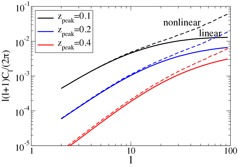
that peaks at ${z_{\rm peak}}=2z_{0}$. In Fig. 3 we show the angular power spectra for ${z_{\rm peak}}=0.1,0.2$ and $0.4$; the angular spectra are of course smooth because they correspond to matter overdensity projected along the line of sight. This figure also shows that nonlinearities enter at $\ell\gtrsim 20$; in our analysis, we are interested in reconstructing $\ell$ of a few, and thus it is sufficient to use the linear angular power spectra.

Figure 3: The theoretical angular power spectra calculated using the radial number density function $n(z)$ from the SDSS for different redshifts at which the radial number density of objects peaks. See Appendix C for details of the calculation.

Details of how we first generate a smooth projected matter density map, and from it the distribution of galaxies on the sky, are spelled out in Appendix D. In brief, starting with the choice of the form of the galaxy density $dN/dz$ and its peak value ${z_{\rm peak}}$, we use the calculated theoretical $C_{\ell}$ at $\ell\leq 50$ to generate a set of random $a_{\ell m}$ with zero mean and variance $C_{\ell}$. We then use the HEALPix healpix routine alm2map to generate a smooth density map.

Next, we generate a galaxy catalog with $N_{g}$ galaxies consistent with the smooth map; details are described in Appendix D. Starting with the coefficients $C_{\ell}$, we generate 100 random sets of $a_{\ell m}$ coefficients, and from each we produce 3 realizations of the corresponding galaxy catalog. This gives us a total of 300 realizations of galaxies on which we base the statistics. This number was smaller than we might have liked, because the galaxy generation step is time consuming for large $N_{g}$ ($\gtrsim 10^{8}$). We found, however, that this number of realizations produced sufficiently accurate results.

V.3 Testing the reconstruction accuracy

We now investigate how the accuracy of the estimated quantities of interest (i.e. the $a_{\ell m}$ and the multipole vectors) depends on the characteristics of the survey – its depth, and the sky density of tracer objects. We follow the procedure outlined in deOliveiraCosta:2006zj and optimally reconstruct the full-sky $a_{\ell m}$ from each mock catalog using the method described in Sec. V. The corresponding MVs are subsequently extracted from the $a_{\ell m}$ using the publicly available code MV_code .

Figure 4: Reconstruction of the coefficients $a_{\ell m}$ for $\ell=2-4$ for 300 realizations with $N_{g}=10^{4}$ (top row), $N_{g}=10^{5}$ (middle row) and $10^{6}$ (bottom row). We show results for three HEALPix map resolutions: pixelizations of ${N_{\rm side}}$ = 4 (blue), 8 (black) and 16 (red). The total number of pixels on the full sky is ${N_{\rm pix}}=12\times{N_{\rm side}}^{2}$. The true underlying $a_{\ell m}$ are shown by the dotted line. An increase in resolution (i.e. higher ${N_{\rm side}}$) improves the accuracy of the reconstruction only for mock catalogs of size $N_{g}=10^{6}$ and higher.

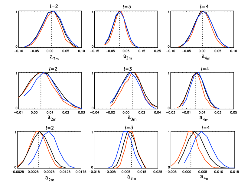
Sufficiently fine pixelization. In our approach, one performs counts-in-cells of galaxies on the sky. To test effects of finite resolution imposed by pixelization, we consider a single realization of a galaxy survey with $N_{g}$ objects and reconstruct the $a_{\ell m}$ using different values of the HEALPix parameter ${N_{\rm side}}$, where the number of pixels is ${N_{\rm pix}}=12{N_{\rm side}}^{2}$ (the angular size of a pixel is roughly $\theta_{\rm pix}\approx 60^{\circ}/{N_{\rm side}}$).

Figure 4 shows the reconstructed $a_{\ell m}$ for three choices of ${N_{\rm side}}$ and for 300 realizations of mock catalogs with $N_{g}=10^{5}$, $10^{6}$ and $10^{7}$ objects. The width of each distribution encapsulates the variance on the measurement of the multipole coefficient and remains relatively unchanged as the pixelization varies. Clearly, for catalogs with smaller galaxy density (i.e. larger shot noise), an increase from ${N_{\rm side}}=4$ to ${N_{\rm side}}=8$ improves the accuracy of the reconstruction only marginally, rendering ${N_{\rm side}}=8$ sufficient to guarantee that the contribution to noise is dominated by the shot noise for a survey with $10^{5}$ objects (which is reduced with increased resolution). For larger number density catalogs ($N_{g}=10^{6}$ in the Figure), a higher pixelization of ${N_{\rm side}}=16$ does make a slight improvement in the $a_{\ell m}$ estimation but not enough to warrant the additional computation time. For the rest of the analysis, ${N_{\rm side}}=8$ will be used.

Figure 5: Effects of the number density of LSS tracers. Histograms of the dot product of the true and reconstructed MVs, $\cos(\Theta^{(\ell,i)})=v^{(\ell,i)}\cdot v_{\rm true}^{(\ell,i)}$, from $300$ realizations for surveys with $N_{g}=10^{4}$ (top row), $N_{g}=10^{6}$ (middle row), and $N_{g}=10^{8}$ (bottom row). We assume a fixed pixelization level of ${N_{\rm side}}=8$, and the radial distribution of objects ${z_{\rm peak}}=0.2$. An improvement in accuracy is indicated by a closer proximity to $1$, at which the MVs are reconstructed perfectly. The narrowing of the histograms suggests a considerably better recovery of the MVs as the survey size is increased.

Sky density of objects. The projected sky density of objects will vary dramatically between different classes of objects. For example, using all galaxies as tracers will provide higher counts than using only the luminous red galaxies, and those in turn have a much higher density than quasars or gamma-ray bursts. More accurate reconstruction of the underlying density field is expected to be revealed from catalogs with a larger numbers of objects. Therefore, the number of tracer objects in the survey is likely to play an important role in the precision of our tests.

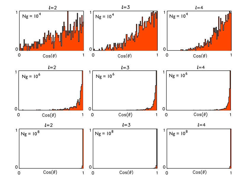
Let us examine the effect of the available number of sources in the reconstruction accuracy of multipole vectors $v^{({\ell},i)}$. To do that, we compare the MVs $v^{(\ell,i)}$ obtained from the reconstructed $a_{\ell m}$ to those $v_{\rm true}^{(\ell,i)}$ which corresponds to the $a_{\ell m}$ used to generate the density map of the mock catalog. The results are quantified by the angles $\Theta^{(\ell,i)}$

$$\cos\left(\Theta^{(\ell,i)}\right)=v_{\rm true}^{(\ell,i)}\cdot v^{(\ell,i)}$$ (27)

from $300$ realizations as a function of the total number of galaxies $N_{g}$. Fig. 5 shows the histograms for catalogs increasing with $N_{g}=10^{4},10^{6}$ and $10^{8}$. The loss of accuracy is gauged by how much $\cos(\Theta^{(\ell,i)})$ deviates from perfect reconstruction where its value is unity. The widths of the one-sided distributions decrease dramatically as the number of objects in the survey $N_{g}$ increases, indicating substantial increase in the ability of a galaxy catalog to represent the underlying density field. The rapid degradation in the accuracy of estimated MVs for $N_{g}\ll 10^{6}$ already hints that large catalogs may be required to test SI reliably.

Figure 6: Effects of the sky cut. Histogram of the dot products of the true and reconstructed MVs $\cos(\Theta^{(\ell,i)})=v_{\rm true}^{(\ell,i)}\cdot v^{(\ell,i)}$, from $300$ realizations when the following areas of the sky are removed: $0$ (top row), $\pm 4.5^{\circ}$ (middle row), and $\pm 9^{\circ}$ (bottom row). The second and third case correspond to $f_{\rm sky}\simeq 0.92$ and $0.84$ respectively. The pixelization level is fixed at ${N_{\rm side}}=8$ and we assume a survey with $N_{g}=10^{6}$ objects which radial distribution of tracers that peaks at ${z_{\rm peak}}=0.2$.

Figure 7: Effects of the survey depth. Histogram of the dot products of the true and reconstructed MVs $\cos(\Theta^{(\ell,i)})=v_{\rm true}^{(\ell,i)}\cdot v^{(\ell,i)}$ from $300$ realizations of a full sky for a surveys with ${z_{\rm peak}}=0.1,0.2$ and $0.4$ (top to bottom rows). The adopted pixelization is ${N_{\rm side}}=8$ and the total number of sources is $N_{g}=10^{6}$.

Figure 8: Summary of all effects. Plot of the average angle between the reconstructed and input MVs, $\Theta^{(\ell,i)}=\arccos\left(v_{\rm true}^{(\ell,i)}\cdot v^{(\ell,i)}\right)$ as a function of $N_{g}$, with error bars indicating the $16-84$ percentile ranges for different choices of ${z_{\rm peak}}$; ${z_{\rm peak}}=0.1$ (left column), ${z_{\rm peak}}=0.2$ (middle column) and ${z_{\rm peak}}=0.4$ (right column) for $\ell=2$ (top row), $\ell=3$ (middle row) and $\ell=4$ (bottom row). The different colors indicate different sky masks: $0^{\circ}$ (black), $\pm 4.5^{\circ}$ (blue) and $\pm 9^{\circ}$ (red).

Sky cut. It is likely that, for most tracer objects of the large-scale structure, parts of the sky will have to be masked either to incomplete observations, or to the presence of point sources. The removal of data from part of the sky will inevitably degrade the accuracy of the reconstruction of the $a_{\ell m}$, multipole vectors, and any other statistics. In Ref. Copi:2003kt , it was shown that accurate reconstruction of the MVs of the CMB temperature anisotropy (to about a degree or better) requires a galaxy cut no larger than a few degrees. Here we perform a similar analysis for the MVs of the large-scale structure.

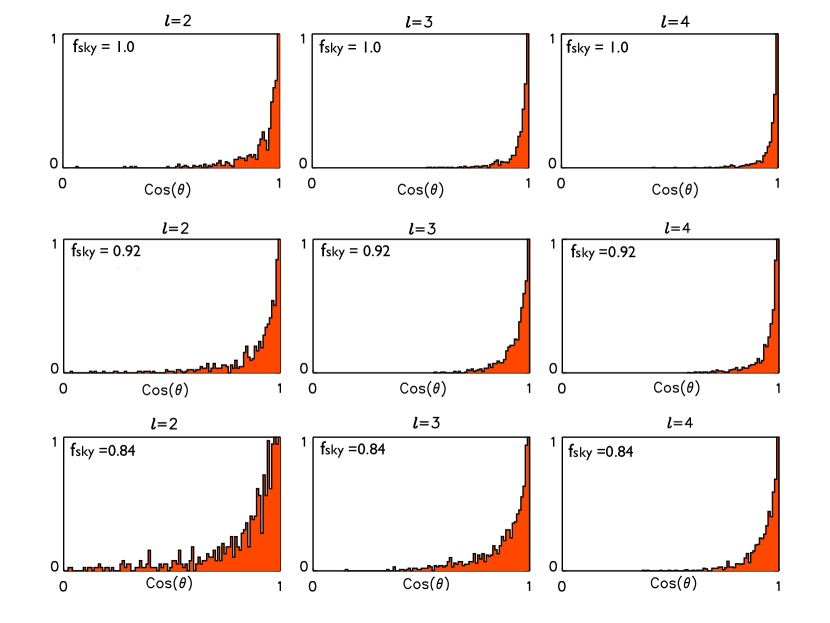
We assume the following isolatitude cuts: $0^{\circ}$, $\pm 4.5^{\circ}$ and $\pm 9^{\circ}$, corresponding respectively to the full sky, 8%, and 16% of the sky area masked. Given that our test skies are statistically isotropic, the fiducial orientation of the cuts is irrelevant. And while the fact that isolatitude cuts are assumed is certainly a simplifying assumption, we do not expect that the azimuthally uneven cut with roughly the same area will lead to very different results. We leave the analysis with cuts with more general geometries for future work when cuts motivated by specific surveys will be used.

Fig. 6 shows histograms of the dot products of the true input MVs and the reconstructed MVs $\cos(\Theta^{(\ell i)})=v_{\rm true}^{(\ell,i)}\cdot v^{(\ell,i)}$ for 300 realizations of a galaxy survey with $N_{g}=10^{6}$ and the three different cuts. When only part of the sky is observed, mixing of the higher multipoles, $\ell\gtrsim 1/\theta_{\rm cut}$, with those describing the reconstructed sky (${\bf a}$) is introduced. The reconstruction method implemented here accounts for this mode-mixing in the reconstructed multipoles ${\bf a}$ at the cost of larger error bars, indicated by the increase in the widths of the histograms as $f_{\rm sky}$ decreases.

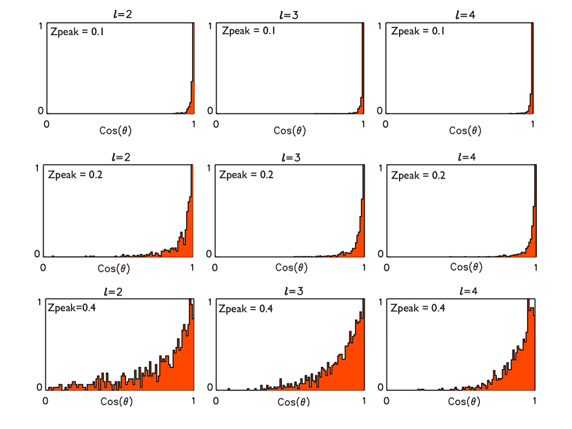
Survey depth. Reconstruction also depends on the depth of the survey, which we here parametrize with the peak of the redshift distribution of sources ${z_{\rm peak}}$. While a deeper survey enables a larger effective representative volume of the universe from which to test statistical isotropy, it turns out that the angular power spectrum has a lower amplitude for a deeper survey; see Fig. 3. This is why deeper surveys lead to worsening in the reconstruction of the multipole vectors. Fig. 7 shows a marked increase in the error of the reconstructions with increasing redshifts of the source distribution.

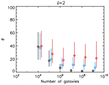
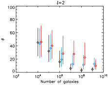
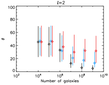
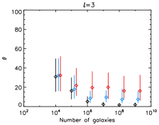
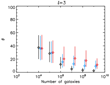
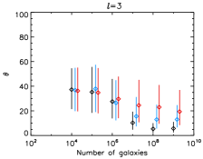
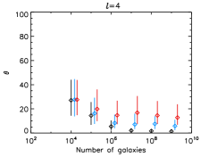
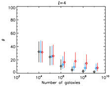
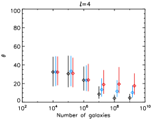
This analysis illustrates the role of the additional factors which must be taken into account when adapting CMB tests of SI to the case of LSS. The full set of results are summarized in Fig. 8. One interesting observation is that the accuracy of the reconstruction is comparable for all $\ell$ when the entire sky is observed (black lines) but deteriorates from high to low $\ell$ (bottom to top panel) when part of the sky is surveyed (blue and red lines). This trend becomes more apparent as $f_{\rm sky}$ decreases from $0.92$ (blue) to $0.84$ (red). Furthermore, we find that the reconstruction accuracy plateaus at around $N_{g}=10^{6}$-$10^{8}$ in almost all cases considered, with little improvement at higher source densities. Overall, and perhaps as expected, we find the primary limiting factor to be incomplete sky coverage and not the density of the sources.

VI Recovering Evidence of Alignments

The robustness tests from the previous section imply a certain accuracy in reconstructing the multipole vectors out of noisy data. We now test how this accuracy translates into detection of the violations of SI.

For the sake of definitiveness, let us assume a purely phenomenological model where the sky has a quadrupole and octopole that are perfectly planar. That is, we assume that the quadrupole and octopole $a_{\ell m}$ coefficients are pure $a_{22}$ and $a_{33}$. [Any mix of $a_{22}^{RE}$, $a_{22}^{IM}$, $a_{33}^{RE}$ and $a_{33}^{IM}$ will do, since the real/imaginary mixing only affects the azimuthal structure in the plane.] We first create Monte Carlo realizations of skies that have this type of perfect alignment at $\ell=2,3$ while having other $a_{\ell m}$ drawn from the usual Gaussian distributions. We then apply our reconstruction of the sky temperature, and thus the multipole vectors, and study whether the alignment is observable.

If the aligned model has planar structures — as observed on our sky by WMAP — then it is advantageous to study the directions and magnitudes of the mutual cross products of multipole vectors, which are referred to as the “oriented area” vectors: CHSS_review

$$w^{(\ell,i,j)}\equiv v^{(\ell,i)}\times v^{(\ell,j)}.$$ (28)

Let us illustrate how one could search for planar alignments represented by the near-collinear oriented area vectors that we use as an example. Let us define a new statistic

$$B_{\rm signal}=\underset{\hat{d}}{\min}\left[\frac{1}{N_{\rm pairs}}\sum_{\ell=2}^{{\ell_{\rm max}}}\sum_{j=2}^{\ell}\sum_{\begin{subarray}{c}i=1\end{subarray}}^{j-1}\left(1-\frac{\mid w^{(\ell,i,j)}\cdot\hat{d}\mid}{\mid w^{(\ell,i,j)}\mid}\right)^{2}\right]^{1/2}$$ (29)

where ${\ell_{\rm max}}=3$ and the minimization is over all possible directions $\hat{d}$. For our alignment model, a perfect reconstruction of multipole vectors would imply that all oriented area vectors are collinear, so that $B_{\rm signal}=0$. In the presence of the uncertainty in the reconstruction, however, the oriented area vectors $w^{(\ell,i,j)}$ will generally not be aligned, and $B_{\rm signal}$ will be greater than zero but presumably small. Finally, for a statistically isotropic sky, we expect that the oriented areas do not preferentially lie close to any single direction $\hat{d}$, so that $B_{\rm signal}^{\rm unaligned}\gg B_{\rm signal}^{\rm aligned}$.

We generate 50,000 Monte Carlo realizations of the perfectly aligned skies with purely planar quadrupole and octopole as described above and higher multipoles consistent with statistically isotropy. We also generate 50,000 statistically isotropic skies. In each case, we reconstruct the coefficients $a_{\ell m}$, and the corresponding multipole vectors, as described in Sec. V. We consider one case where the survey has $10^{6}$ galaxies whose distribution peaks at ${z_{\rm peak}}=0.1$, and another case with $10^{9}$ galaxies with ${z_{\rm peak}}=0.4$, representing examples of a shallow and a deep survey respectively. For the reconstruction, we use ${N_{\rm side}}=8$, and a sky cut of either $0^{\circ}$ (i.e. $f_{\rm sky}=1$) or $\pm 9^{\circ}$ (i.e. $f_{\rm sky}\simeq 0.84$).

Figure 9: Detectability of perfectly aligned quadrupole and octopole in a mock survey using the $B_{\rm signal}$ statistic (see Eq. 29). Each histogram is based on 50,000 Monte Carlo realizations. Solid lines shows survey with $N_{g}=10^{6}$ objects and the radial distribution that peaks at ${z_{\rm peak}}=0.1$, while the dashed lines show a survey with $N_{g}=10^{9}$ and ${z_{\rm peak}}=0.4$ (the ’unaligned’ case, shown with the red solid line, is independent of the presence of the cut and the values of ${z_{\rm peak}}$ and $N_{g}$). The grey region covers values of $B_{\rm signal}$ which correspond to the bottom 5% of the isotropic (i.e. unaligned) sky cases. We find that 98-99% of the aligned skies without the galactic cut (and for either of the two ${z_{\rm peak}}$ cases) lie below this value — in other words, it is roughly at the 20:1 odds that the value of $B_{\rm signal}$ found below this value favors the aligned model.

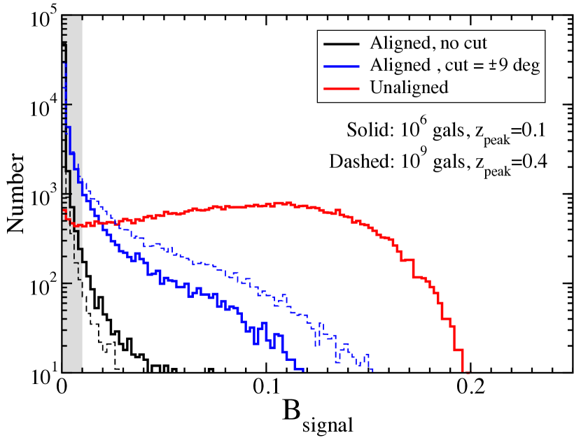
The histogram of the statistics $B_{\rm signal}$ is shown in Fig. 9. As expected, the values of $B_{\rm signal}$ for the aligned skies are preferentially smaller than for the unaligned (i.e. isotropic) realizations. The shaded region covers values of $B_{\rm signal}$ which correspond to the bottom 5% of the isotropic (i.e. unaligned) sky cases; therefore, finding $B_{\rm signal}$ below this value would indicate a $\sim 2\sigma$ evidence for this particular alignment. We find that 98-99% of the aligned sky realizations without the galactic cut (and for either of the two ${z_{\rm peak}}$ cases) lie below this value of $B_{\rm signal}$, and so it is with this probability that one would find a $\sim 2\sigma$ evidence for the alignment. With the $\pm 9^{\circ}$ sky cut, evidence for alignments will be weaker, and the $2\sigma$ evidence can be made in 65% (${z_{\rm peak}}=0.4$, $N_{g}=10^{9}$) or 85% (${z_{\rm peak}}=0.1$, $N_{g}=10^{6}$) percent of the realizations of the aligned model.

These results are encouraging, given that we did not optimize over the choice of the statistic to detect the assumed alignment. In this exploratory paper we do not study the issue of detectability any further, perform a complete likelihood analysis, or study more specific models for the alignment; this is left for future work.

VII Discussion and future work

In this paper we have proposed to apply the statistical tools developed for studies of the CMB to conduct tests of the statistical isotropy (SI) of large-scale structure. We considered the projected (i.e. two-dimensional) density field provided by a galaxy catalog, and expanded it into multipole moments analogously to how the CMB temperature field is conventionally analyzed. Each multipole can be decomposed into a set of $\ell$ multipole vectors $\left\{\hat{v}^{(\ell,i)}i=1...,\ell\right\}$ and a scalar $A_{(\ell)}$. These vectors represent all phase information contained in the projected density field, and enable a variety of tests of directionality in the galaxy distribution. We developed an algorithm to reconstruct the full-sky multipole vectors out the the cut-sky galaxy catalog, while carefully accounting for the signal and noise specific to the galaxy maps. Note that galaxies are not the only feasible tracers of the LSS; clusters of galaxies, gamma-ray bursts, X-ray and radio sources, and other tracers could also be potentially very useful in testing the SI.

In this work we have concentrated on the large scales, in particular only considering the multipoles $\ell=2-4$; extension to smaller scales is in principle straightforward. Because LSS surveys typically do not typically cover the full sky, we have implemented the reconstruction of the full-sky (recently applied to CMB temperature maps in deOliveiraCosta:2006zj ). Exactly to what extent this reconstruction effectively assumes SI has recently been debated CHSS_review ; Efstathiou2009 ; Pontzen_Peiris ; Aurich_Lustig . The issue of how to test SI with reconstructed full-sky information that explicitly does not assume SI on relevant scales is an important problem in its own right, and we leave it for future work.

Unlike the CMB temperature anisotropy field, which comes from a single, well-defined redshift, galaxy surveys mapping the local universe are diverse in their source density and redshift range and, like the CMB maps, can also cover different areas of the sky. We explored the impact of each of these survey properties and found the primary limiting factor to be incomplete sky coverage. Even a modest Galactic plane cut increases the noise in the reconstruction due to mode mixing. We find that if a significant fraction ($\sim 16\%$) of the sky is not surveyed, the accuracy quickly becomes limited by the uncertainty in the reconstructed full-sky properties due to the cut, with little improvement in the errors achieved by increasing the number of objects beyond $10^{6}$.

We also find that the accuracy of the reconstruction is comparable for all $\ell$ when the entire sky is observed, but deteriorates from high to low $\ell$ when part of the sky is surveyed; see Fig. 8. The reconstruction accuracy typically plateaus at around $N_{g}=10^{6}$-$10^{8}$, suggesting that there is an intrinsic limit on how well the multipole vectors can be recovered. Furthermore, the recovery of the multipole vectors is more accurate in a catalogs with sources at lower redshifts due to a higher power in those cases (see Fig. 3).

Using a statistic constructed to detect planar alignments, we tested for violations of SI in Monte Carlo simulations of isotropic skies, and of skies in which the quadrupole and octopole are perfectly aligned. We found a $98\%$ chance of making a $2\sigma$ detection of this particular alignment using a galaxy catalog with $10^{6}$ sources of mean redshift $z=0.1$, detected over the entire sky. This likelihood drops to $85\%$ when $16\%$ of the sky is masked out. Similarly, for the ${z_{\rm peak}}=0.4$, $N_{g}=10^{9}$ survey, we find the probabilities of 99% ($f_{\rm sky}=1$) and 65% ($f_{\rm sky}=0.84$) of finding a $2\sigma$ detection of this particular alignment. Note, however, that we have not optimized over the choice of the detection statistic, nor considered any physical models for the alignment, so actual success in detecting such anomalies may well be different from these numbers.

The next decade or two will see a dramatic improvement in the galaxy data on largest observable scales. For example, the Wide-field Infrared Survey Explorer (WISE), currently observing, will provide an all-sky survey from 3.5 to 23 $\mu m$ about a thousand times more sensitive than IRAS, and should produce a very large number of objects out to redshift of $z\sim 3$. Clearly, data provided by surveys such as WISE in the infrared, and perhaps other radio, X-ray and optical surveys, would be perfect targets to test the SI with the multipole vectors. Such wide and deep surveys could even start to probe the scales probed by the large-angle CMB; for example, it is possible (though somewhat unlikely) that LSS can confirm or refute the missing large-angle primordial power favored by the CMB in this scenario Gibelyou:2010qe .

Quite possibly the biggest challenge in studying realistic surveys may be understanding the details of any given survey, and culling out a representative subsample of objects that can be used for tests of isotropy. Fortunately, since we are primarily interested in large scale information, we do not need to worry as much about other commonly found systematic effects in galaxy surveys due to nonlinear clustering. However, it is clear that details of the selection function for each survey will need to be known fairly accurately, as spatial or temporal variations in depth of observations can masquerade as evidence for violations of SI.

In conclusion, we hope that multipole vectors will do the same for the LSS maps that they did for the CMB: provide a novel and useful way to quantify anisotropies on the sky. In the case of the CMB, this has led to a variety of new tests of the SI with interesting results. We hope that the applications to real LSS surveys will be equally fruitful.

Appendix A Conventions

The temperature on the sky can be decomposed in terms of spherical harmonics

$${\delta T\over T}(\theta,\phi)=\sum_{\ell,m}a_{\ell m}Y_{\ell m}(\theta,\phi).$$ (30)

Spherical harmonics $Y_{\ell m}$ can be defined in terms of the associated Legendre polynomials $P_{\ell m}$

$$Y_{\ell m}\left(\theta,\phi\right)=\sqrt{\frac{(2\ell+1)(\ell-m)!}{4\pi(\ell+m)!}}P_{\ell m}\left(\cos\theta\right)e^{im\phi}.$$ (31)

For computing convenience, we wish to to work with real numbers only. Breaking up the spherical harmonics $Y_{\ell m}$ and the coefficients $a_{\ell m}$ into real and imaginary parts

$$a_{\ell m} = a_{\ell m}^{Re}+ia_{\ell m}^{Im}$$ (32)

$$Y_{\ell m} = Y_{\ell m}^{Re}+iY_{\ell m}^{Im}$$ (33)

For negative $m$

$$a_{\ell-m} = (-1)^{m}a_{\ell m}^{*}=(-1)^{m}\left(a_{\ell m}^{Re}-ia_{\ell m}^{Im}\right)$$ (34)

$$Y_{\ell-m} = (-1)^{m}Y_{\ell m}^{*}=(-1)^{m}\left(Y_{\ell m}^{Re}-iY_{\ell m}^{Im}\right).$$ (35)

The contribution to the sum $\sum_{m}a_{\ell m}Y_{\ell m}$ from a single value of $|m|$ is

$$a_{\ell m}Y_{\ell m}+a_{\ell-m}Y_{\ell-m}=$$ (36)

$$\left\{\begin{array}[]{cl}2\left(a_{\ell m}^{Re}Y_{\ell m}^{Re}-a_{\ell m}^{Im}Y_{\ell m}^{Im}\right)&(m\neq 0)\\[5.69046pt] a_{\ell 0}Y_{\ell 0}&(m=0)\\[5.69046pt] \end{array}\right.$$ (39)

We define the following: $Y_{\ell m}\equiv|Y_{\ell m}|\cos\left(m\phi\right)+i|Y_{\ell m}|\sin\left(m\phi\right)$. Following deOliveiraCosta:2006zj , we define

1. $Y^{1}_{\ell m}\equiv\sqrt{2}\,|Y_{\ell m}|\,\cos\left(m\phi\right)\hfill~{}\left(\text{for}~{}m>0\right)$

2. $Y^{2}_{\ell m}\equiv\sqrt{2}\,|Y_{\ell m}|\,\sin\left(m\phi\right)\hfill\left(\text{for}~{}m<0\right)$

3. $Y^{3}_{\ell m}\equiv|Y_{\ell m}|\,\hfill\left(\text{for}~{}m=0\right)$

We then define the following parameters:

1. $b^{1}_{\ell m}\equiv\sqrt{2}a_{\ell m}^{RE}\hfill\left(\text{for}~{}m>0\right)$

2. $b^{2}_{\ell m}\equiv-\sqrt{2}a_{\ell m}^{IM}\hfill\left(\text{for}~{}m<0\right)$

3. $b^{3}_{\ell m}\equiv a_{\ell m}\hfill\left(\text{for}~{}m=0\right)$

Hence, we can obtain the right-hand side of Eq. (39) using the following summation over real quantities, $b_{\ell m}^{1}Y_{\ell m}^{1}+b^{2}_{\ell m}Y^{2}_{\ell m}$ (for $m\neq 0$) or $b_{\ell m}^{3}Y_{\ell m}^{3}$ (for $m=0$).

Appendix B The covariance matrix

The reconstruction method described in Sec. V.1 requires the calculation of the covariance matrix ${\bf C}$. We discuss this in detail given the various subtleties which require attention.

Firstly, we consider the sources of detector noise encapsulated in ${\bf N}$. The reconstruction of the underlying function $\nu(\Omega)$ from a galaxy survey introduces two types of noise. The nature of the sampling process means that in an actual catalog, the number of objects in the i^th pixel will not be $n_{i}$ defined in Eq. (13), but rather an integer $\tilde{n}_{i}$. This difference is due to shot noise, encompassed in the parameter $\nu_{i}$, given by

$$\nu_{i}=\frac{\tilde{n}_{i}-n_{i}}{\bar{n}}.$$ (40)

In the same way, the average number of objects per pixel will not be $\bar{n}$ but rather $\tilde{n}$, given by

$$\tilde{n}\equiv\frac{1}{{N_{\rm pix}}}\sum_{i=1}^{N_{p}}\tilde{n}_{i}.$$ (41)

The above $\tilde{n}$ is the survey mean and is taken to be our best estimate of the ensemble mean $\bar{n}$. We estimate the density contrast $\Delta_{i}$ using the mean number density of the survey on its largest scales Tegmark:1997cx

$$\tilde{\Delta}_{i}=\frac{\tilde{n}_{i}-\tilde{n}}{\tilde{n}}.$$ (42)

This procedure forces our estimates of the fluctuations on the largest scale of the survey to zero, an effect sometimes called the ’integral constraint’. Following EDSGC , a parameter $\epsilon$ is introduced to account for the fractional difference between the survey mean and the ensemble mean

$$\epsilon\equiv\frac{\tilde{n}-\bar{n}}{\bar{n}}.$$ (43)

Using the fact that $\Delta_{i}\equiv(n_{i}-{\bar{n}})/{\bar{n}}$ – see Eq. (15) – we can relate our estimate $\tilde{\Delta}_{i}$ to the true value $\Delta_{i}$ in terms of $\epsilon$ and $\nu_{i}$ as

$$\tilde{\Delta}_{i}=\frac{\Delta_{i}+\nu_{i}-\epsilon}{1+\epsilon}.$$ (44)

This equation relates the measured density contrast $\tilde{\Delta}_{i}$ to the theoretically predicted density contrast $\Delta_{i}$.

We now wish to calculate the statistical properties of catalog density contrast $\tilde{\Delta}_{i}$, in particular, its mean and covariance. We need to express these in terms of statistical properties of the ensemble density contrast $\Delta_{i}$.

It will be useful to rewrite

$$\tilde{\Delta}_{i}\simeq\left(\Delta_{i}+\nu_{i}-\epsilon\right)\left(1-\epsilon+\epsilon^{2}+{\cal O}(\epsilon^{3})\right)$$ (45)

where the following hold

$$\langle\nu_{i}\nu_{j}\rangle = \delta_{ij}\frac{(1+\Delta_{i})}{\bar{n}}+{\cal O}(\bar{N}_{g}^{-2})$$

$$\langle\epsilon\rangle = 0$$

$$\langle\epsilon^{2}\rangle = \frac{1}{\bar{N}_{g}}$$

$$\langle\nu_{i}\rangle = 0$$

$$\langle\nu_{i}\epsilon\rangle = \frac{1}{\bar{N}_{g}}$$

$$\langle\nu_{i}\epsilon^{2}\rangle = 0$$

$$\langle\nu_{i}\nu_{j}\epsilon^{2}\rangle = \frac{\delta_{ij}(1+\Delta_{i})}{\bar{N}_{g}\bar{n}}+{\cal O}(\bar{N}_{g}^{-2})$$ (46)

Note that the expectation value is $\langle\Delta_{i}\rangle=\Delta_{i}$ and not zero, as in the case of the ensemble. Putting this together we find

$$\langle\tilde{\Delta}_{i}\rangle=\Delta_{i}\left(1+\frac{1}{\bar{N}_{g}}\right).$$ (47)

Furthermore, we find that

$$\langle\tilde{\Delta}_{i}\tilde{\Delta}_{j}\rangle = \Delta_{i}\Delta_{j}\langle\left(1+3\epsilon^{2}\right)\rangle-2\left(\Delta_{i}\langle\nu_{j}\epsilon\rangle+\Delta_{j}\langle\nu_{i}\epsilon\rangle\right)$$ (48)

$$+ \langle\nu_{i}\nu_{j}(1+3\epsilon^{2})\rangle+2\left(\Delta_{i}+\Delta_{j}\right)\langle\epsilon^{2}\rangle-\langle\left(\nu_{i}+\nu_{j}\right)\epsilon\rangle$$

$$+ \langle\epsilon^{2}\rangle+{\cal O}(\bar{N}_{g}^{-2})$$

$$= \Delta_{i}\Delta_{j}\left(1+\frac{3}{\bar{N}_{g}}\right)+\frac{\delta_{ij}(1+\Delta_{i})}{\bar{n}}\left(1+\frac{3}{\bar{N}_{g}}\right)$$

$$- \frac{1}{\bar{N}_{g}}+{\cal O}(\bar{N}_{g}^{-2}).$$

The covariance matrix of $\tilde{\Delta}_{i}$ is therefore:

$$C_{ij} \equiv \langle\tilde{\Delta}_{i}\tilde{\Delta}_{j}\rangle-\langle\tilde{\Delta}_{i}\rangle\langle\tilde{\Delta}_{j}\rangle$$ (49)

$$= \frac{1}{\bar{N}_{g}}\left(\Delta_{i}\Delta_{j}-1\right)+\frac{\delta_{ij}(1+\Delta_{i})}{\bar{n}}$$

$$+ {\cal O}(\bar{N}_{g}^{-2}).$$

We need to write both $\langle\tilde{\Delta}_{i}\rangle$ and $C_{ij}$ in terms of the $a_{\ell m}$. Using Eq. (18), we can write

$$\langle\tilde{\Delta}_{i}\rangle=\sum_{\ell=2}^{{\ell_{\rm max,rec}}}\sum_{m}a_{\ell m}Y_{\ell m}(\Omega_{i})\left(1+\frac{1}{\bar{N}_{g}}\right).$$ (50)

Notice that we have truncated the sum over $a_{\ell m}$ at ${\ell_{\rm max,rec}}$ which is the last multipole that we reconstruct. The $a_{\ell m}$ at higher $\ell$ are replaced by their expectation values in the ensemble of universes, in which $\langle a_{\ell m}\rangle=0.$ We treat the covariance matrix $C_{ij}$ in a similar fashion and replace $a_{\ell m}a_{\ell^{\prime}m^{\prime}}$ by its expectation value in the ensemble of universes:

$$\langle a_{\ell m}a_{\ell^{\prime}m^{\prime}}\rangle=\delta_{\ell\ell^{\prime}}\delta_{mm^{\prime}}{\cal C}_{\ell}\,.$$ (51)

We follow deOliveiraCosta:2006zj in their reconstruction of the $a_{\ell m}$, and reconstruct a limited range of multipoles, $2\leq\ell\leq{\ell_{\rm max,rec}}$. This procedure treats the higher multipoles ${\ell_{\rm max,rec}}+1\leq\ell\leq{\ell_{\rm max,tot}}$ as “noise” to the reconstructed multipoles’“signal”. Following this logic, we split the pixel density fluctuations into the suitably chosen signal and noise parts

$$\tilde{\Delta}_{i} = \frac{\Delta_{i}+\left(\nu_{i}-\epsilon\right)}{1+\epsilon}$$ (52)

$$\simeq \Delta_{i}\left(1-\epsilon+\epsilon^{2}\right)+\frac{\nu_{i}-\epsilon}{1+\epsilon}$$

$$= \sum_{\ell=2}^{{\ell_{\rm max,rec}}}b_{\ell m}Y_{\ell m}(\Omega_{i})$$

$$+ \left[\sum_{\ell={\ell_{\rm max,rec}}+1}^{\ell_{max}}\sum_{m}b_{\ell m}Y_{\ell m}(\Omega_{i})+\left(\epsilon^{2}-\epsilon\right)\Delta_{i}+\frac{\nu_{i}-\epsilon}{1+\epsilon}\right]$$

$$\equiv \sum_{\ell=2}^{{\ell_{\rm max,rec}}}\sum_{m}b_{\ell m}Y_{\ell m}(\Omega_{i})+{\cal N}_{i}.$$

where

$${\cal N}_{i}=\sum_{\ell={\ell_{\rm max,rec}}+1}^{{\ell_{\rm max,tot}}}\sum_{m}b_{\ell m}Y_{\ell m}(\Omega_{i})+\left(\epsilon^{2}-\epsilon\right)\Delta_{i}+\frac{\nu_{i}-\epsilon}{1+\epsilon}$$

and where we take ${\ell_{\rm max,tot}}=50$. Note that the $a_{\ell m}$ have been recast in new variables denoted $b_{\ell m}$ defined in Appendix A in order to simplify the calculation. In the above, ${\cal N}_{i}$ is the noise in the i^th pixel. The first term in Eq. (B) is the contribution from leakage from multipoles which are not reconstructed, while the next two terms are due to shot noise arising from the sampling process. Taking expectation value of Eq. (B) we get

$$\langle{\cal N}_{i}\rangle = \sum_{\ell={\ell_{\rm max,rec}}+1}^{{\ell_{\rm max,tot}}}\sum_{m}b_{\ell m}Y_{\ell m}(\Omega_{i})+\langle\epsilon^{2}\rangle\Delta_{i}$$ (53)

$$+ \Big{\langle}\frac{\nu_{i}}{1+\epsilon}\Big{\rangle}-\Big{\langle}\frac{\epsilon}{1+\epsilon}\Big{\rangle}$$

$$= \frac{\Delta_{i}}{\bar{N}_{g}}+\sum_{\ell={\ell_{\rm max,rec}}+1}^{{\ell_{\rm max,tot}}}\sum_{m}b_{\ell m}Y_{\ell m}(\Omega_{i}).$$ (54)

As usual, $a_{\ell m}$ terms with $\ell>{\ell_{\rm max,rec}}$ are neglected as they are unknown and will not be reconstructed. Our treatment of the unknown true underlying perturbation $\Delta_{i}$ is limited and we merely replace it with our current best estimate in an iterative process:

$$\langle{\cal N}_{i}\rangle^{(p)}\simeq\frac{1}{\bar{N}_{g}}\sum_{\ell=2}^{{\ell_{\rm max,rec}}}b_{\ell m}Y_{\ell m}(\Omega_{i})+\sum_{\ell=2}^{{\ell_{\rm max,rec}}}\sum_{m}b_{\ell m}^{(p)}Y_{\ell m}(\Omega_{i})$$ (55)

where $(p)$ numbers the iterative step. At the $0^{th}$ iteration we use $b_{\ell m}^{(0)}=0$, which is then replaced by estimates of $b_{\ell m}$ in successive iterations until convergence is achieved.

The covariance of the noise is given by

$$\langle{\cal N}_{i}{\cal N}_{j}\rangle^{(p)}=$$ (56)

$$\Bigg{\langle}\Bigg{(}\sum_{\ell={\ell_{\rm max,rec}}+1}^{\ell_{max}}\sum_{m}b_{\ell m}Y_{\ell m}(\Omega_{i})+\left(\epsilon^{2}-\epsilon\right)\Delta_{i}$$

$$+ \frac{\nu_{i}}{1+\epsilon}-\frac{\epsilon}{1+\epsilon}\Bigg{)}$$

$$\times\Bigg{(}\sum_{\ell^{\prime}={\ell_{\rm max,rec}}+1}^{\ell_{max}}\sum_{m^{\prime}}b_{\ell^{\prime}m^{\prime}}Y_{\ell^{\prime}m^{\prime}}(\Omega_{j})+\left(\epsilon^{2}-\epsilon\right)\Delta_{j}$$

$$+ \frac{\nu_{j}}{1+\epsilon}-\frac{\epsilon}{1+\epsilon}\Bigg{)}\Bigg{\rangle}.$$

Replacing $\langle b_{\ell m}b_{\ell^{\prime}m^{\prime}}\rangle$ by its expectation value in the ensemble of Universes (for $\ell\geq{\ell_{\rm max,rec}}$, ${\cal C}_{\ell}\delta_{\ell\ell^{\prime}}\delta_{mm^{\prime}}$), and $\langle b_{\ell m}\rangle$ by its expectation value (i.e. zero) we find

$$\langle{\cal N}_{i}{\cal N}_{j}\rangle^{(p)} = \sum_{\ell={\ell_{\rm max,rec}}+1}^{\ell_{max}}\frac{2\ell+1}{4\pi}{\cal C}_{\ell}P_{\ell}(\cos\theta_{ij})$$

$$+ [\langle\epsilon^{2}\rangle\left(1+\Delta_{i}^{(p)}+\Delta_{j}^{(p)}+\Delta_{i}^{(p)}\Delta_{j}^{(p)}\right)$$

$$- \langle\epsilon\nu_{j}\rangle(\Delta_{i}^{(p)}+1)-\langle\epsilon\nu_{i}\rangle(\Delta_{j}^{(p)}+1)$$

$$+ \langle\nu_{i}\nu_{j}\rangle+3\langle\epsilon^{2}\nu_{i}\nu_{j}\rangle]$$

$$= \sum_{\ell={\ell_{\rm max,rec}}+1}^{\ell_{max}}\frac{2\ell+1}{4\pi}{\cal C}_{\ell}P_{\ell}(\cos\theta_{ij})$$

$$+ \left[\frac{\delta_{ij}(1+\Delta_{i}^{(p)})}{\bar{n}}\left(1+\frac{3}{\bar{N}_{g}}\right)+\frac{1}{\bar{N}_{g}}(\Delta_{i}^{(p)}\Delta_{j}^{(p)}-1)\right]$$

$$+ {\cal O}\left(\frac{1}{\bar{N}_{g}^{2}}\right).$$

Since $\langle{\cal N}_{i}\rangle\langle{\cal N}_{j}\rangle^{(p)}={\cal O}(1/\bar{N}_{g}^{2})$, $C_{ij}^{(p)}=\langle{\cal N}_{i}{\cal N}_{j}\rangle^{(p)}$. For clarity, we separate the covariance matrix out into its two contributions;

$$C^{(p)}_{ij} = S_{ij}^{(p)}+N_{ij}^{(p)}$$

where

$$S_{ij}^{(p)} = \sum_{\ell={\ell_{\rm max,rec}}+1}^{\ell_{max}}\frac{2\ell+1}{4\pi}{\cal C}_{\ell}P_{\ell}(\cos\theta_{ij})$$ (57)

$$N_{ij}^{(p)} = \left[\frac{\delta_{ij}(1+\Delta_{i}^{(p)})}{\bar{n}}\left(1+\frac{3}{\bar{N}_{g}}\right)+\frac{1}{\bar{N}_{g}}(\Delta_{i}^{(p)}\Delta_{j}^{(p)}-1)\right].$$

In the first evaluation we use $\Delta_{i}^{(p)}=\tilde{\Delta}_{i}$. Once the first set of reconstructed $b_{\ell m}$ are extracted, they will be used to update $\Delta_{i}^{(p)}=\sum_{\ell=2}^{{\ell_{\rm max,rec}}}b_{\ell m}Y_{\ell m}(\Omega_{i})$ for the subsequent iterations. Note that the value of the $C_{\ell}$ used in the computation of the signal matrix $S$ is not crucial: error in the estimation of the angular power spectrum will merely mean that more iterations will be required for convergence.

As discussed above, the true average number of galaxies per pixel is unknown and can only be estimated by the mean calculated from the survey. This assumption $\tilde{N}_{g}=\bar{N_{g}}$ however artificially suppresses the estimates of the power on large scales and is accounted for by the factor of $1/\bar{N}_{g}$ in the last term of Eq. (B). Comparing the expression in Eq. (B) with the covariance matrix calculated for the CMB in deOliveiraCosta:2006zj , we find that they are in agreement if we bear in mind that the case of the CMB effectively corresponds to the case where $N_{g}\rightarrow\infty$

Appendix C The theoretical angular power spectrum $C_{\ell}$

Equation (22) shows that an estimate of the angular power spectrum $C_{\ell}$ is required for our reconstruction. We now show how to calculate the angular power spectrum of a large-scale structure survey (for pioneering works on this, see Baugh_Efstathiou ; EDSGC ; Efstathiou_Moody ). We only consider a single, vanilla best-fit $\Lambda$CDM cosmological model, as the cosmological model dependence of the $C_{\ell}$ is not expected to affect the results.

The angular power spectrum in harmonic space can be related to its counterpart in Fourier space via

$$C_{\ell}=\int^{\infty}_{0}K_{\ell}(k)P(k)k^{2}dk$$ (58)

where, as shown in EDSGC , $K_{\ell}$ is an integral kernel given by $\frac{2}{\pi}f_{\ell}^{2}(k)$ where $f_{\ell}$ is the Bessel transform of the radial selection function $f(r)=g(r)h(r)$. Here $g(r)$ is the radial probability distribution of galaxies

$$g(r)\propto\frac{dN}{dr}=\frac{dN/dz}{dr/dz}=H(z)\,\frac{dN}{dz}$$ (59)

where $dN/dz$ is the radial redshift distribution of objects in the survey. The objects which constitute potential catalogs are biased tracers of dark matter; while this bias primarily depends on the object’s mass, for definitiveness we assume $b=1$. The function $h(r)$ which accounts for this galaxy bias as well as clustering, is therefore assumed to be unity. This means that the power spectrum above is measured at a radial distance of $r\sim\ell/k$. Hence,

$$f_{\ell}(k)\equiv\int^{\infty}_{0}j_{\ell}(kr)f(r)dr=\int^{\infty}_{0}j_{\ell}(kr(z))\frac{dN}{dz}dz,$$ (60)

where $j_{\ell}(kr)$ is the spherical Bessel function of order $\ell$. As mentioned in the text, we assume the distribution of objects of the form $dN/dz\equiv n(z)\propto z^{2}\exp(-z/z_{0})$ that peaks at ${z_{\rm peak}}=2z_{0}$. The power spectrum $P(k)$ is approximated to be scale-invariant with $P(k)\propto k^{n_{s}}$ where we adopt $n_{s}=0.96$ and normalization consistent with WMAP data.

So far we have assumed the linear clustering regime, which will dominate on the large scales that we are interested in. Nevertheless, it is important to check what the role of nonlinearities will be. To that effect, we adopt the following simple correction formula proposed in Cole:2005sx relating the linear and nonlinear power spectra

$$P_{\rm nl}(k)=b^{2}\frac{1+Q_{\rm nl}k^{2}}{1+A_{\rm nl}k}P(k)$$ (61)

where $A_{\rm nl}=1.4$. The factor $Q_{\rm nl}$ is determined from the galaxy catalog itself, and we adopt the value obtained by the Sloan Digital Sky Survey Luminous Red Galaxies of $Q_{\rm nl}=31$ Tegmark:2006az . The linear and nonlinear angular power spectra of surveys with ${z_{\rm peak}}=0.1$, $0.2$ and $0.4$ are shown in Fig. 3.

Appendix D Mock catalog generation

A density map is constructed in the following way:

1. The theoretical power spectrum (based on the SDSS power spectrum) is calculated for a $\Lambda$CDM Universe for a given set of cosmological parameters. The amplitude of the spectrum is determined by the redshift distribution of sources, $dN/dz$, which is assumed to be a Gaussian peaking at ${z_{\rm peak}}$. The theoretical power spectra for the three cases considered (${z_{\rm peak}}=0.1,0.2$ and $0.4$) are shown in Fig. 3.

2. A set of $a_{\ell m}$ are drawn randomly from a distribution centered at zero with variance $C_{\ell}^{th}$, so that $a_{\ell m}\in N(0,C_{\ell})$. The corresponding power spectrum is denoted $C_{\ell}^{\rm realiz}\equiv\sum_{m}|a_{\ell m}|^{2}$.

3. The HEALpix routine alm2map is used to generate a density map of $12{N_{\rm side}}^{2}$ pixels from the input $a_{\ell m}$. Initially we use a high pixelization of ${N_{\rm side}}=64$ to produce a smoother density field.

The density map generated in the above manner is used as the basis for constructing each realization of a galaxy survey as follows;

1. The density map is populated with $N_{g}$ “galaxies” (i.e. points) so that the fraction of sources allocated to each pixel represents the underlying average fluctuation in density around the mean. Given that we would like to investigate the impact of the number of galaxies in the survey and sky coverage of the survey separately, regardless of the sky cut we first create full-maps with the number of galaxies of $N_{g}/f_{\rm sky}$, so that the total number of galaxies on the cut sky will be a fixed $N_{g}$.

2. In order to speed up the computation (which requires inversion of matrices of size ${N_{\rm pix}}\times{N_{\rm pix}}$ where ${N_{\rm pix}}=12{N_{\rm side}}^{2}$), we downgrade the maps to a lower resolution using the HEALPix routine udgrade. The cost of the reduced accuracy in the reconstruction due to the downgrading process is considered in Sec. V.3.

3. In cases where we are simulating a masked sky, we remove (i.e. set to zero counts) galaxies in the isolatitude cut of $\pm 4.5^{\circ}$ or $\pm 9^{\circ}$.

4. Elements of the noise matrix ${\cal N}$ are initially estimated using the measured map. In the subsequent iterations, the elements are computed using the reconstructed $a_{\ell m}$. We perform three such iterations of the reconstruction and update the $a_{\ell m}$ at each step. Convergence is tested.

The above process is repeated 300 times to produce a set of realizations from which the necessary statistics can be calculated.

References

- (1) J. C. Mather, E. S. Cheng, R. E. Eplee, Jr., R. B. Isaacman, S. S. Meyer, R. A. Shafer, R. Weiss, E. L. Wright, C. L. Bennett, N. W. Boggess, E. Dwek, S. Gulkis, M. G. Hauser, M. Janssen, T. Kelsall, P. M. Lubin, S. H. Moseley, Jr., T. L. Murdock, R. F. Silverberg, G. F. Smoot, and D. T. Wilkinson, ApJL 354, L37 (May 1990)
- (2) J. C. Mather, E. S. Cheng, D. A. Cottingham, R. E. Eplee, Jr., D. J. Fixsen, T. Hewagama, R. B. Isaacman, K. A. Jensen, S. S. Meyer, P. D. Noerdlinger, S. M. Read, L. P. Rosen, R. A. Shafer, E. L. Wright, C. L. Bennett, N. W. Boggess, M. G. Hauser, T. Kelsall, S. H. Moseley, Jr., R. F. Silverberg, G. F. Smoot, R. Weiss, and D. T. Wilkinson, Astrophys. J. 420, 439 (Jan. 1994)
- (3) D. N. Spergel et al. (WMAP), ApJS 148, 175 (2003), astro-ph/0302209
- (4) D. Spergel et al., ApJS 170 (2007), astro-ph/0603449
- (5) E. Komatsu et al. (WMAP), Astrophys. J. Suppl. 192, 18 (2011), arXiv:1001.4538 [astro-ph.CO]
- (6) G. Hinshaw, A. J. Branday, C. L. Bennett, K. M. Gorski, A. Kogut, C. H. Lineweaver, G. F. Smoot, and E. L. Wright, ApJL 464, L25+ (Jun. 1996), astro-ph/9601061
- (7) C. J. Copi, D. Huterer, D. J. Schwarz, and G. D. Starkman, Phys. Rev. D 75, 023507 (Jan. 2007), astro-ph/0605135
- (8) C. J. Copi, D. Huterer, D. J. Schwarz, and G. D. Starkman, MNRAS 399, 295 (Oct. 2009), arXiv:0808.3767
- (9) D. Sarkar, D. Huterer, C. J. Copi, G. D. Starkman, and D. J. Schwarz, Astropart.Phys. 34, 591 (2011), arXiv:1004.3784 [astro-ph.CO]
- (10) A. Hajian, ArXiv Astrophysics e-prints astro-ph/0702723 (Feb. 2007), astro-ph/0702723
- (11) E. F. Bunn and A. Bourdon, Phys. Rev. D 78, 123509 (2008), arXiv:arXiv:0808.0341
- (12) D. J. Schwarz, G. D. Starkman, D. Huterer, and C. J. Copi, Phys. Rev. Lett. 93, 221301 (Mar. 2004), astro-ph/0403353
- (13) M. Tegmark, A. de Oliveira-Costa, and A. J. Hamilton, Phys. Rev. D68, 123523 (Dec. 2003)
- (14) K. Land and J. Magueijo, Phys. Rev. Lett. 95, 071301 (2005)
- (15) A. Yoho, F. Ferrer, and G. D. Starkman, Phys. Rev. D83, 083525 (2011), arXiv:1005.5389 [astro-ph.CO]
- (16) H. K. Eriksen, F. K. Hansen, A. J. Banday, K. M. Górski, and P. B. Lilje, Astrophys. J. 605, 14 (2004), astro-ph/0307507
- (17) F. K. Hansen, P. Cabella, D. Marinucci, and N. Vittorio, Astrophys. J. 607, L67 (2004), astro-ph/0402396
- (18) H. K. Eriksen, A. J. Banday, K. M. Gorski, F. K. Hansen, and P. B. Lilje, Astrophys. J. 660, L81 (2007), astro-ph/0701089
- (19) F. K. Hansen, A. J. Banday, K. M. Gorski, H. K. Eriksen, and P. B. Lilje, Astrophys. J. 704, 1448 (2009), arXiv:arXiv:0812.3795 [astro-ph]
- (20) J. Hoftuft et al., Astrophys. J. 699, 985 (2009), arXiv:arXiv:0903.1229 [astro-ph.CO]
- (21) C. Raeth et al.(2010), arXiv:1012.2985 [astro-ph.CO]
- (22) C. J. Copi, D. Huterer, D. J. Schwarz, and G. D. Starkman, Mon. Not. Roy. Astron. Soc. 367, 79 (2006), astro-ph/0508047
- (23) C. L. Bennett et al., Astrophys. J. Suppl. 192, 17 (2011), arXiv:1001.4758 [astro-ph.CO]
- (24) D. Huterer, New Astron. Rev. 50, 868 (2006), arXiv:astro-ph/0608318
- (25) C. J. Copi, D. Huterer, D. J. Schwarz, and G. D. Starkman, Adv.Astron. 2010, 847541 (2010), arXiv:1004.5602 [astro-ph.CO]
- (26) C. M. Hirata, JCAP 0909, 011 (2009), arXiv:arXiv:0907.0703 [astro-ph.CO]
- (27) A. R. Pullen and C. M. Hirata, JCAP 1005, 027 (2010), arXiv:1003.0673 [astro-ph.CO]
- (28) S. Ando and M. Kamionkowski, Phys. Rev. Lett. 100, 071301 (2008), arXiv:arXiv:0711.0779 [astro-ph]
- (29) C. Gordon, W. Hu, D. Huterer, and T. M. Crawford, Phys. Rev. D72, 103002 (2005), arXiv:astro-ph/0509301
- (30) L. Ackerman, S. M. Carroll, and M. B. Wise, Phys. Rev. D75, 083502 (2007), arXiv:astro-ph/0701357
- (31) J. F. Donoghue, K. Dutta, and A. Ross, Phys. Rev. D80, 023526 (2009), arXiv:astro-ph/0703455
- (32) C. Armendariz-Picon, JCAP 0709, 014 (2007), arXiv:arXiv:0705.1167 [astro-ph]
- (33) A. E. Gumrukcuoglu, C. R. Contaldi, and M. Peloso, JCAP 0711, 005 (2007), arXiv:arXiv:0707.4179 [astro-ph]
- (34) D. C. Rodrigues, Phys. Rev. D77, 023534 (2008), arXiv:arXiv:0708.1168 [astro-ph]
- (35) A. R. Pullen and M. Kamionkowski, Phys. Rev. D76, 103529 (2007), arXiv:0709.1144 [astro-ph]
- (36) C. Pitrou, T. S. Pereira, and J.-P. Uzan, JCAP 0804, 004 (2008), arXiv:arXiv:0801.3596 [astro-ph]
- (37) A. L. Erickcek, M. Kamionkowski, and S. M. Carroll, Phys. Rev. D78, 123520 (2008), arXiv:arXiv:0806.0377 [astro-ph]
- (38) A. L. Erickcek, C. M. Hirata, and M. Kamionkowski, Phys. Rev. D80, 083507 (2009), arXiv:arXiv:0907.0705 [astro-ph.CO]
- (39) R. Battye and A. Moss, Phys. Rev. D80, 023531 (2009), arXiv:arXiv:0905.3403 [astro-ph.CO]
- (40) N. E. Groeneboom and H. K. Eriksen, Astrophys. J. 690, 1807 (2009), arXiv:arXiv:0807.2242 [astro-ph]
- (41) D. Hanson and A. Lewis, Phys. Rev. D80, 063004 (2009), arXiv:arXiv:0908.0963 [astro-ph.CO]
- (42) N. E. Groeneboom, L. Ackerman, I. K. Wehus, and H. K. Eriksen, Astrophys.J. 722, 452 (2010), arXiv:0911.0150 [astro-ph.CO]
- (43) D. Hanson, A. Lewis, and A. Challinor, Phys. Rev. D81, 103003 (2010), arXiv:1003.0198 [astro-ph.CO]
- (44) A. de Oliveira-Costa, M. Tegmark, M. Zaldarriaga, and A. Hamilton, Phys. Rev. D69, 063516 (2004), astro-ph/0307282
- (45) C. J. Copi, D. Huterer, and G. D. Starkman, Phys. Rev. D70, 043515 (2004), arXiv:astro-ph/0310511
- (46) J. C. Maxwell, A Treatise on Electricity and Magnetism, 3rd ed., Vol. I (Clarendon Press, London, 1891)
- (47) G. Katz and J. Weeks, Phys. Rev. D70, 063527 (2004), astro-ph/0405631
- (48) M. R. Dennis, J. Phys. A: Math. Gen. 38, 1653 (Feb. 2005)
- (49) C. J. Copi, “Freely downloadable multipole vector code,” http://www.phys.cwru.edu/projects/mpvectors/#code
- (50) J. R. Weeks, astro-ph/0412231(Dec. 2004)
- (51) R. C. Helling, P. Schupp, and T. Tesileanu, Phys. Rev. D 74, 063004 (Sep. 2006), astro-ph/0603594
- (52) G. Hinshaw et al. (WMAP), ApJS 170, 288 (2007), astro-ph/0603451
- (53) M. R. Dennis, J. Phys. A: Math. Gen. 37, 9487 (Oct. 2004)
- (54) C. L. Bennett et al., ApJS 148, 97 (2003), astro-ph/0302208
- (55) H. K. Eriksen, A. J. Banday, K. M. Górski, and P. B. Lilje, Astrophys. J. 612, 633 (2004), astro-ph/0403098
- (56) M. Tegmark and G. Efstathiou, MNRAS 281, 1297 (aug 1996), arXiv:astro-ph/9507009
- (57) F. K. Hansen, A. J. Banday, H. K. Eriksen, K. M. Gorski, and P. B. Lilje, Astrophys. J. 648, 784 (2006), arXiv:astro-ph/0603308
- (58) A. de Oliveira-Costa and M. Tegmark, Phys. Rev. D74, 023005 (2006), astro-ph/0603369
- (59) M. Tegmark, Phys. Rev. D56, 4514 (1997), arXiv:astro-ph/9705188
- (60) D. Huterer, M. Takada, G. Bernstein, and B. Jain, Mon. Not. Roy. Astron. Soc. 366, 101 (2006), arXiv:astro-ph/0506030
- (61) K. M. Górski, E. Hivon, A. J. Banday, B. D. Wandelt, F. K. Hansen, M. Reinecke, and M. Bartelmann, Astrophys. J. 622, 759 (Apr. 2005)
- (62) G. Efstathiou, Y. Ma, and D. Hanson(Nov. 2009), arXiv:arXiv:0911.5399
- (63) A. Pontzen and H. V. Peiris, Phys.Rev. D81, 103008 (2010), arXiv:1004.2706 [astro-ph.CO]
- (64) R. Aurich and S. Lustig, Mon.Not.Roy.Astron.Soc. 411, 124 (2011), arXiv:1005.5069 [astro-ph.CO]
- (65) C. Gibelyou, D. Huterer, and W. Fang, Phys.Rev. D82, 123009 (2010), arXiv:1007.0757 [astro-ph.CO]
- (66) M. Tegmark(1997), arXiv:astro-ph/9708021
- (67) D. Huterer, L. Knox, and R. C. Nichol, Astrophys. J. 555, 547 (Jul. 2001), astro-ph/0011069
- (68) C. M. Baugh and G. Efstathiou, MNRAS 267, 323 (Mar. 1994)
- (69) G. Efstathiou and S. J. Moody, MNRAS 325, 1603 (Aug. 2001), astro-ph/0010478
- (70) S. Cole et al. (The 2dFGRS), Mon. Not. Roy. Astron. Soc. 362, 505 (2005), arXiv:astro-ph/0501174
- (71) M. Tegmark et al. (SDSS), Phys. Rev. D74, 123507 (2006), arXiv:astro-ph/0608632