Heat conduction in disordered harmonic lattices with energy conserving noise

Abstract

We study heat conduction in a harmonic crystal whose bulk dynamics is supplemented by random reversals (flips) of the velocity of each particle at a rate $\lambda$. The system is maintained in a nonequilibrium stationary state(NESS) by contacts with white noise Langevin reservoirs at different temperatures. We show that the one-body and pair correlations in this system are the same (after an appropriate mapping of parameters) as those obtained for a model with self-consistent reservoirs. This is true both for the case of equal and random(quenched) masses. While the heat conductivity in the NESS of the ordered system is known explicitly, much less is known about the random mass case. Here we investigate the random system, with velocity flips. We improve the bounds on the Green-Kubo conductivity obtained by Bernardin bernardin09 . The conductivity of the 1D system is then studied both numerically and analytically. This sheds some light on the effect of noise on the transport properties of systems with localized states caused by quenched disorder.

I Introduction

We consider heat transport in mass disordered harmonic lattices with stochastic bulk dynamics. For the $1D$ disordered harmonic lattice without stochasticity the effect of localization due to disorder leads, in the presence of pinning, to an exponential decay of the heat current as a function of the length dhar01 ; dharleb08 . In the absence of pinning the conductivity depends on the boundary conditions either growing as $\sqrt{N}$ or decaying as $1/\sqrt{N}$ casher71 ; rubin71 . The situation is very different when one adds stochasticity to the dynamics. Bernardin bernardin09 obtained finite positive upper and lower bounds on the Green-Kubo conductivity of a harmonic lattice with periodic boundary conditions subjected to stochastic dynamics which conserves energy but not momentum.

In this paper we study the heat flux of such a disordered harmonic system, both pinned and unpinned, connected to white noise Langevin type heat reservoirs with different temperatures at the two ends. The stochastic part of the bulk dynamics consists of random reversals of each particle’s velocity at a rate $\lambda$. The analytical as well as accurate numerical tractability of this model makes it a good test system to address the problem of the effect of noisy dynamics on transport properties of disordered systems. To the extent that stochastic dynamics affect phonon-phonon interactions in some rough sense similar to anharmonicity, this may also teach us something about the effects of the latter. The effect of interactions on localization and transport in disordered systems has generated much interest and has been studied both for the case of electron and phonon transport basko08 ; vadim07 ; pikovsky07 ; kopidakis07 ; dharleb08 ; dhar08 ; bernardin09 ; mulansky09 ; vadim09 ; basko10  . A study by two of us dharleb08 of the heat conductivity of the disordered 1D pinned lattice with anharmonicity found that a small amount of anharmonicity was sufficient to cause a transition to a diffusive regime with a finite value of $\kappa$. The question of whether the transition from an insulator to conductor occurs at zero or some finite small value of anharmonicity remains an open problem. For the noisy dynamics on the other hand bernardin09 shows that an arbitrarily small noise leads to normal transport. The work of basko10 suggests a transition at zero nonlinearity for classical systems (the quantum situation may be different).

There have been some recent studies delfini08 ; lepri09 on the NESS of ordered harmonic chains with noisy dynamics conserving both energy and momentum, and with white noise Langevin baths at different temperatures at the two ends. It was shown in these studies that the time-evolution of the pair-correlations formed closed sets of equations. This closure is true also for the energy conserving model that we study. In addition we show a mapping of the steady state equations for one-body and pair-correlation functions to that of the self-consistent reservoirs model first introduced by Bolsterli etal BRV70 ; RV75 and recently solved exactly for the ordered case by Bonetto etal BLL04 .

The plan of the paper is as follows. In sec II we define the model precisely and show the mapping to the model with self-consistent reservoirs. In sec III we use the method of Bernardin bernardin09 to obtain improved lower and upper bounds for the Green-Kubo thermal conductivity of the random mass system. In sec IV we present results from numerical calculations as well as nonequilibrium simulations for the dependence of the heat flux in the random mass case on system size and on noise strength. Both the pinned and unpinned system are studied. For the pinned case conductivity decreases with the strength of the binding and increases with strength of the noise. For the unpinned case we study the effect of boundary conditions (BCs) . Finally we conclude with a discussion of the nature of the NESS for this model. While it is easily checked that the NESS is not strictly Gaussian, we find that the one particle momentum and position distributions are very close to Gaussian distribution. Furthermore their values at different sites or of momentum and position at the same site are essentially uncorrelated.

II Noisy dynamics and self-consistent reservoirs

The results in this section apply in any dimension. For simplicity of notation we consider here explicitly the one dimensional case; a harmonic chain with the Hamiltonian:

$$H = \sum_{l=1,N}\left[\frac{p_{l}^{2}}{2m_{l}}+k_{o}\frac{q_{l}^{2}}{2}\right]+\sum_{l=2,N}k\frac{(q_{l}-q_{l-1})^{2}}{2}+k^{\prime}\left[\frac{q_{1}^{2}}{2}+\frac{q_{N}^{2}}{2}\right]$$

$$= \frac{1}{2}\left[p\hat{M}^{-1}p+q\hat{\Phi}q\right]~{},$$

where $\{q_{l},p_{l}\}$ denote the position and momenta of the particles. We have used the notation $p=(p_{1},p_{2},...,p_{N}),~{}q=(q_{1},q_{2},...,q_{N})$ and $\hat{M}$ and $\hat{\Phi}$ are $N\times N$ matrices corresponding to masses and forces respectively. When $k_{o}>0$ we have the pinned case and set $k^{\prime}=k$. In the unpinned case, $k_{o}=0$, we consider fixed, $k^{\prime}>0$, and free, $k^{\prime}=0$, boundary conditions.

The system’s evolution has a deterministic part described by the Hamiltonian above and a stochastic part consisting of two different processes: (i) every particle is subjected to a noise which flips its momentum, i.e. for the $l^{\rm th}$ particle the transition $p_{l}\to-p_{l}$ occurs with a rate $\lambda$, (ii) the particles at the boundaries $l=1$ and $l=N$ are attached to heat baths with Langevin dynamics at temperatures $T_{L}$ and $T_{R}$ respectively. Thus the end particles have additional terms in their equation of motion of the form $-\gamma p_{\alpha}/m_{\alpha}+(2\gamma T_{\alpha})^{1/2}\eta_{\alpha}(t)$, for $\alpha=1,N$, with $\langle\eta_{\alpha}(t)\eta_{\alpha^{\prime}}(t^{\prime})\rangle=\delta_{\alpha,\alpha^{\prime}}~{}\delta(t-t^{\prime})$, $\gamma$ is the friction constant and $T_{1}=T_{L},~{}T_{N}=T_{R}$ are the bath temperatures.

The master equation describing the time evolution of the full phase space probability density is therefore given by:

$$\frac{\partial P(x)}{\partial t}=\sum_{l,m}{\hat{a}}_{lm}x_{m}\frac{\partial}{\partial x_{l}}P+\sum_{l,m}\frac{\hat{d}_{lm}}{2}\frac{\partial^{2}P}{\partial x_{l}\partial x_{m}}+\lambda\sum_{l}[P(...,-p_{l},...)-P(...,p_{l},...)]~{},$$ (2)

where $x=(q_{1},q_{2},\ldots,q_{N},p_{1},p_{2},\ldots,p_{N})=(x_{1},x_{2},\ldots,x_{2N})$ and $\hat{a}$ and $\hat{d}$ are $2N\times 2N$ matrices given by:

$$\hat{a}=\left(\begin{array}[]{cc}0&-\hat{M}^{-1}\\ \hat{\Phi}&\hat{M}^{-1}\hat{\Gamma}^{-1}\end{array}\right)~{}~{}~{}~{}~{}\hat{d}=\left(\begin{array}[]{cc}0&0\\ 0&2\hat{T}\hat{\Gamma}\end{array}\right)~{}.$$ (7)

Here $\hat{T}$ and $\hat{\Gamma}$ are diagonal matrices with diagonal elements given by $\hat{T}_{ll}=T_{L}\delta_{l,1}+T_{R}\delta_{l,N}$ and $\hat{\Gamma}_{ll}=\gamma(\delta_{l,1}+\delta_{l,N})$ respectively. Similar to the case studied in delfini08 we also find that the equations for the one-body and pair correlation functions of the system are closed. (In fact there are closed equations for each order of the correlation.) We define the vector $\rho$ , $\rho_{l}=<x_{l}>,\,l=1,2\dots 2N$ and the pair correlation matrix

$$\hat{c}=\left(\begin{array}[]{cc}\hat{u}&\hat{z}\\ \hat{z}^{T}&\hat{v}\end{array}\right).$$ (10)

where the $N\times N$ matrices $\hat{u},\hat{z}$ and $\hat{v}$ are given by $\hat{u}_{lm}=\langle q_{l}q_{m}\rangle~{},\hat{v}_{lm}=\langle p_{l}p_{m}\rangle$ and $\hat{z}_{lm}=\langle q_{l}p_{m}\rangle$ . It follows then from Eq. (2) $\rho$ and $\hat{c}$ satisfy the following equations of motion:

$$\frac{d\rho}{dt} = -\hat{a}\rho+\left(\frac{d\rho}{dt}\right)_{col}~{},$$

$$\frac{d\hat{c}}{dt} = -\hat{a}\hat{c}-\hat{c}\hat{a}^{T}+\hat{d}+\left(\frac{d\hat{c}}{dt}\right)_{col}~{},$$ (11)

where the last terms in the above two equations arise from the flip dynamics and are given by:

$$\left(\frac{d\rho}{dt}\right)_{col} = -2\lambda\left(\begin{array}[]{c}0\\ \langle p\rangle\end{array}\right)$$ (14)

$$\left(\frac{d\hat{c}}{dt}\right)_{col} = -2\lambda\left(\begin{array}[]{cc}0&\hat{z}\\ \hat{z}^{T}&2(\hat{v}-\hat{v}_{D})\end{array}\right)~{},$$ (17)

and $\hat{v}_{D}$ is a diagonal matrix with matrix elements $[\hat{v}_{D}]_{ll}=\hat{v}_{ll}=\langle p_{l}^{2}\rangle$.

In the steady state, $d\rho/dt=0$ which implies $\rho=0$. Setting $d\hat{c}/dt=0$ gives the following set of equations for the pair correlations in the NESS:

$$\hat{z}^{T}=-\hat{M}\hat{z}\hat{M}^{-1}~{},$$

$$\hat{v}=\frac{1}{2}(\hat{M}\hat{u}\hat{\Phi}+\hat{\Phi}\hat{u}\hat{M})+\frac{1}{2}(\hat{M}\hat{z}\hat{\Gamma}\hat{M}^{-1}+\hat{M}^{-1}\hat{\Gamma}\hat{z}^{T}\hat{M})~{},$$

$$(\hat{M}\hat{u}\hat{\Phi}-\hat{\Phi}\hat{u}\hat{M})+(\hat{M}\hat{z}\hat{\Gamma}\hat{M}^{-1}-\hat{M}^{-1}\hat{\Gamma}\hat{z}^{T}\hat{M})+2\lambda(\hat{M}\hat{z}-\hat{z}^{T}\hat{M})=0~{},$$

$$(\Phi\hat{z}+\hat{z}^{T}\hat{\Phi})+(\hat{M}^{-1}\hat{\Gamma}\hat{v}+\hat{v}\hat{\Gamma}\hat{M}^{-1})+4\lambda(\hat{v}-\hat{v}_{D})=2\hat{T}\hat{\Gamma}~{}.$$ (18)

Using the fact that $\hat{u}$ and $\hat{v}$ are symmetric matrices we have $N^{2}+N(N+1)$ unknown variables and there are that many independent equations above.

Now consider the case of heat conduction across a harmonic chain with Hamiltonian given by  (II) and self consistent reservoirs attached to all sites. This is in addition to the two end reservoirs at fixed temperatures $T_{L}$ and $T_{R}$. Each of the side reservoirs is a Langevin bath with a friction constant $\gamma^{\prime}_{l}$ and a temperature $T^{\prime}_{l}$, $l=1,2,...N$, which is self-consistently fixed by the condition that there is no net flow of energy into the reservoir BLL04 . The stochastic equations of motion of this system are:

$$\frac{dp_{1}}{dt} = -\Phi_{1m}q_{m}-\frac{\gamma}{m_{1}}p_{1}-\frac{\gamma^{\prime}_{1}}{m_{1}}p_{1}+(2\gamma T_{L})^{1/2}\eta_{1}(t)+(2\gamma^{\prime}_{1}T^{\prime}_{1})^{1/2}\zeta_{1}(t)$$

$$\frac{dp_{l}}{dt} = -\Phi_{lm}q_{m}-\frac{\gamma^{\prime}_{l}}{m_{l}}p_{l}+(2\gamma^{\prime}_{l}T^{\prime}_{l})^{1/2}\zeta_{l}(t)~{}~{}l=2,...,N-1~{},$$

$$\frac{dp_{N}}{dt} = -\Phi_{Nm}q_{m}-\frac{\gamma}{m_{N}}p_{N}-\frac{\gamma^{\prime}_{N}}{m_{N}}p_{N}+(2\gamma T_{R})^{1/2}\eta_{N}(t)+(2\gamma^{\prime}_{N}T^{\prime}_{N})^{1/2}\zeta_{N}(t)~{},$$ (19)

where $\eta_{1},\eta_{N}$ and $\zeta_{l},~{}l=1,2,...,N$ are independent Gaussian white noise sources with unit variance. It is immediately established that the probability distribution $P(x)$ in the NESS of this model is a Gaussian. The self consistency condition for zero current into the side reservoirs is given by $T_{l}^{\prime}=\hat{v}_{ll}=\langle p_{l}^{2}\rangle/m_{l}$. Making the identification $\gamma_{l}^{\prime}=2\lambda m_{l}$, it is seen that the equations for the pair-correlations in the steady state corresponding to the above equations are given precisely by Eq. (18).
The self-consistent model was first studied by Bolsterli et al BRV70 who introduced the self-consistent reservoirs as a simple scattering mechanism mimicking anharmonicity and which might ensure local equilibration and the validity of Fourier’s law. The model was later solved exactly by Bonetto et al BLL04 who proved approach to local equilibrium and validity of Fourier’s law for the ordered case, i.e where all the $m_{l}$’s are equal. They also obtained an explicit expression for the thermal conductivity of the system in all dimensions. (see Eq. (24) below)

III Bounds on Green-Kubo conductivity

Bernardin bernardin09 considered a model of a disordered harmonic chain with a stochastic noise that changes the momentum of neighboring particles while keeping the sum of their kinetic energies constant. He obtained an exact result for the Green-Kubo conductivity of an ordered chain and also rigorous upper and lower bounds for the conductivity of disordered chains. Here we use Bernardin’s approach for our model to obtain an exact expression for the ordered chain. We also obtain bounds for the conductivity of the disordered chain which are slightly improved from those of Bernardin’s.

The time evolution of the phase space density is given by Eq. (2) which we rewrite here in a more abstract form for convenience.

$$\frac{\partial P(x)}{\partial t} = LP(x)$$

$${\rm where}~{}~{}L = A+\lambda S$$

$$AP(x) = \sum_{l=1}^{N}[-\frac{p_{l}}{m_{l}}\frac{\partial P(x)}{\partial q_{l}}+\sum_{m=1}^{N}\Phi_{lm}q_{m}\frac{\partial P(x)}{\partial p_{l}}]$$

$$SP(x) = \sum_{l}[P(...,-p_{l},...)-P(...,p_{l},...)]~{}.$$ (20)

The total current which is carried entirely by the Hamiltonian part can be written in the following form:

$${\mathcal{J}}=\frac{k}{2}\sum_{l=1}^{N}\frac{p_{l}}{m_{l}}(q_{l+1}-q_{l-1})\;\;,q_{0}=q_{N}\;,q_{N+1}=q_{1}.$$ (21)

The Green-Kubo expression for the thermal conductivity at temperature T is given by:

$$\kappa_{GK} = \lim_{z\to 0}\lim_{N\to\infty}\frac{1}{NT^{2}}\int_{0}^{\infty}dt~{}e^{-zt}~{}\langle{\mathcal{J}}(0){\mathcal{J}}(t)\rangle$$ (22)

$$= \lim_{z\to 0}\lim_{N\to\infty}\frac{1}{NT^{2}}\int_{0}^{\infty}dt~{}e^{-zt}~{}\int dx~{}{\mathcal{J}}~{}e^{Lt}~{}(~{}{\mathcal{J}}~{}P_{eq}~{})$$

$$= \lim_{z\to 0}\lim_{N\to\infty}\frac{1}{NT^{2}}~{}\langle~{}{\mathcal{J}},~{}(z-L)^{-1}~{}{\mathcal{J}}~{}\rangle~{}.$$

where we have used the notation $\langle f,g\rangle=\int dxf(x)g(x)P_{eq}$ for any two functions $f,g$ of phase space variables $x=(q_{1},\ldots,q_{N},p_{1},\ldots,p_{N})$ and $P_{eq}\sim exp[-\beta H]$ where $H$ is given by the periodicized version of Eq. (II) with $k^{\prime}$ set equal to $0$.

We note the following relations which are easy to prove:

$$A{\mathcal{J}}P_{eq} = \sum_{l,j}\frac{\Phi_{lj}q_{j}}{m_{l}}(q_{l+1}-q_{l-1})P_{eq}$$

$${\rm and}~{}~{}~{}S{\mathcal{J}}P_{eq} = -2{\mathcal{J}}P_{eq}~{}$$ (23)

III.1 Green-Kubo conductivity for equal mass ordered case

For the equal mass case Eq. (23) gives $A{\mathcal{J}}P_{eq}=0$. This is true with or without pinning and corresponds to the fact that for periodic boundary conditions the current operator commutes with the Hamiltonian. Hence we get:

$$\kappa_{GK} = \lim_{z\to 0}\lim_{N\to\infty}\frac{1}{T^{2}N}\int dx~{}{\mathcal{J}}~{}\frac{1}{z+2\lambda}~{}{\mathcal{J}}~{}P_{eq}=\lim_{N\to\infty}\frac{\langle{\mathcal{J}}^{2}\rangle}{2\lambda T^{2}N}~{}.$$

Using the form of ${\mathcal{J}}$ in Eq. (21) we then get:

$$\kappa_{GK} = \frac{kD}{8\lambda m}~{},$$ (24)

$${\rm where}~{}~{}D = \frac{4k}{2k+k_{o}+[(k_{o})(4k+k_{o})]^{1/2}}~{}.$$

This agrees with the result of BLL04 [Eq. (4.18)] where the conductivity was defined as $\kappa=\lim_{N\to\infty}\langle J_{N}\rangle N/(T_{L}-T_{R})$ where $\langle J_{N}\rangle={k}\langle q_{l}p_{l+1}/m_{l+1}\rangle$ ($l=1,2,\ldots,N-1$) is the average heat flux in the NESS of the system with self-consistent reservoirs specified by (19). The mapping between the noisy dynamics model and the self-consistent reservoirs model (with the transformation $\gamma=2\lambda$m ) implies that for our noisy model also $\kappa=\kappa_{GK}$ in the ordered case. Following the methods in BLL04 it is easy to show that the value of $\kappa$ is independent of boundary conditions for the ordered case and while not proven we expect this to be true also for the disordered case for $N\rightarrow\infty$ at fixed $\lambda>0$. In fact there is every reason to believe that whenever the Green-Kubo formula for $\kappa_{GK}$ converges to a finite value when $N\rightarrow\infty$ then it will agree with the conductivity in the NESS defined as $\kappa=\lim_{N\rightarrow\infty}\lim_{T_{L}\rightarrow T_{R}\rightarrow T}N\langle J_{N}\rangle/(T_{L}-T_{R})$.

III.2 Upper and lower bounds on the Green-Kubo conductivity

We now consider the random case where the masses are independently chosen from some distribution. Bernardin’s proof that the conductivity $\kappa_{GK}$ is bounded away from zero and infinity is based on an identity between $\langle{\mathcal{J}},(z-L)^{-1}{\mathcal{J}}\rangle$ and a variational expression (Eq (15) in bernardin09 ),

$$\langle{\mathcal{J}},(z-L)^{-1}{\mathcal{J}}\rangle=Sup\{2\langle u,J\rangle-\langle(z-\lambda S)u,u\rangle-\langle(z-\lambda S)^{-1}Au,Au\rangle\}$$ (25)

where the supremum is carried out over the set of smooth functions $u(q,p)$. The derivation of this formula is straightforward for $A$=0. More generally we can consider a symmetric $L$, e.g one corresponding to a stochastic dynamics satisfying detailed balance with respect to $P_{eq}$. Then we have that $u$ is the solution of the equation $Lu={\mathcal{J}}$ , and both sides of Eq.(25) are equal to $\langle{\mathcal{J}},u\rangle$. For a derivation of Eq. (25) in the case $L=S+A$ with $A$ antisymmetric, see CLTSunder .
Lower bound: Choose a test function $u=\mu\sum_{l}p_{l}(q_{l+1}-q_{l-1})$, where $\mu$ is a variational parameter:

$$\langle u,{\mathcal{J}}\rangle = \frac{k\mu T}{2}\sum_{l}\langle(q_{l+1}-q_{l-1})^{2}\rangle=NT^{2}\frac{\mu D}{2}~{},$$

$$\langle(z-\lambda S)u,u\rangle = (z+2\lambda)\langle u^{2}\rangle=(z+2\lambda)\mu^{2}T\sum_{l}m_{l}\langle(q_{l+1}-q_{l-1})^{2}\rangle~{}.$$

where D is defined in Eq. (24). Denoting by $[...]$ an average over disorder we then get:

$$\left[\langle(z-\lambda S)u,u\rangle\right]=NT^{2}(z+2\lambda)\frac{\mu^{2}D[m]}{k}~{}~{}.$$

Similarly,

$$\langle(z-\lambda S)^{-1}Au,Au\rangle=(z+4\lambda)^{-1}\langle(Au)^{2}\rangle=(z+4\lambda)^{-1}\mu^{2}T^{2}\sum_{l}\left(\frac{1}{m_{l}}-\frac{1}{m_{l+1}}\right)^{2}m_{l}m_{l+1}~{},$$

and averaging over disorder gives

$$\left[\langle(z-\lambda S)^{-1}Au,Au\rangle\right]=2NT^{2}(z+4\lambda)^{-1}\mu^{2}\left([m]\left[\frac{1}{m}\right]-1\right)~{}.$$

Thus we have:

$$\frac{1}{NT^{2}}[\langle{\mathcal{J}},(z-L)^{-1}{\mathcal{J}}\rangle] \geq D\mu-C\mu^{2}$$ (26)

$${\rm where~{}~{}~{}}C = \frac{2\lambda D[m]}{k}+\frac{1}{2\lambda}([m]\left[\frac{1}{m}\right]-1)~{}.$$ (27)

The minimum of the bound occurs at $\mu=D/(2C)$ and this gives:

$$[\kappa_{GK}]\geq\frac{D^{2}}{4C}~{}.$$ (28)

Upper bound: By neglecting the last term in Eq. (25) which is clearly negative, we get the upper bound:

$$\langle{\mathcal{J}},(z-L)^{-1}{\mathcal{J}}\rangle \leq (z+2\lambda)^{-1}\langle{\mathcal{J}}^{2}\rangle=(z+2\lambda)^{-1}T\frac{k^{2}}{4}\sum_{l}\frac{1}{m_{l}}\langle(q_{l+1}-q_{l-1})^{2}\rangle~{}.$$ (29)

$${\rm Hence,}$$

$$~{}~{}[\kappa_{GK}] = \frac{1}{NT^{2}}\left[\langle{\mathcal{J}},(z-L)^{-1}{\mathcal{J}}\rangle\right]\leq\frac{kD}{8\lambda}[\frac{1}{m}]~{}.$$ (30)

Combining (28) and (30) gives:

$$\frac{kD}{8\lambda[m](1+k\frac{[1/m]-1/[m]}{4\lambda^{2}D})}\leq[\kappa_{GK}]\leq\frac{kD}{8\lambda}[\frac{1}{m}]$$ (31)

As $\lambda\rightarrow\infty$, both bounds behave as $1/\lambda$ while for $\lambda\to 0$, the upper bound diverges while the lower bound goes to 0 linearly in $\lambda$. The behavior of $\kappa_{GK}$ and of $\kappa$ in the NESS when $\lambda\rightarrow 0$ after $N\rightarrow\infty$ is thus not determined by these bounds and remains an open problem for both the pinned and unpinned random mass case. What we do know is that, if $\lambda\rightarrow 0$ with N finite then there is a significant difference between the pinned and unpinned cases dharleb08 ; dhar01 . As already noted in the introduction, for the pinned case all phonon modes are localized with a fixed localization length independent of $N$ and the current decays exponentially with system size. In the unpinned case the low frequency modes are extended and the current has a power law decay with an exponent that depends on the boundary conditions used dhar01 , $\kappa_{N}\sim N^{-1/2}$ for fixed BCs casher71 ; AH10 and as $\kappa_{N}\sim N^{1/2}$ for free BCs rubin71 ; verheggen79 . With the addition of the noisy dynamics which conserves energy but not momentum we expect as noted earlier that the conductivity $\kappa$ will be equal to $\kappa_{GK}$ and thus strictly positive for any $\lambda>0$ BernOlla05 . In the following section we evaluate $\langle J_{N}\rangle$ as a function of $\lambda$ and N numerically and via computer simulations, to obtain information about its behavior when $\lambda\rightarrow 0$.

IV Results from numerics and simulations

We study the dependence of the heat current in the NESS on the system size and on the strengths of the disorder and noise. In all our computations we set $k=1$. The masses $\{m_{l}\}$ are chosen from a uniform distribution between $1-\Delta$ to $1+\Delta$. This gives $[m]=1,[{1}/{m}]=1/(2\Delta)\ln[(1+\Delta)/(1-\Delta)]$. The average heat current from site $l$ to $l+1$ is given by $j_{l+1,l}=k\langle q_{l}p_{l+1}/{m_{l+1}}\rangle$. In the steady state this is independent of $l$ and we denote $j_{l+1,l}=\langle J_{N}\rangle$. We note that $\langle J_{N}\rangle=k\hat{z}_{l,l+1}/m_{l+1}$ and hence we can obtain accurate numerical values for the current in the disordered system by solving the equations for the correlation matrix i.e Eqs. (18). This involves solving large dimensional linear matrix equations and we have been able to do this for system sizes less than $N=512$. For larger sizes we performed nonequilibrium simulations and obtained the steady state current by a time average. For small sizes we verified that both methods agreed to very high accuracy. The number for disorder realizations was $100$ for $N\leq 64$, and varied between $2-16$ for larger sizes. The error bars in our data presented below are calculated using the results from different realizations.

IV.1 Pinned case

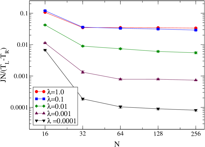
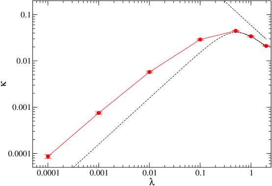
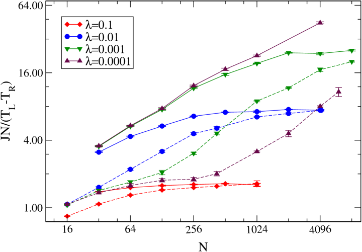
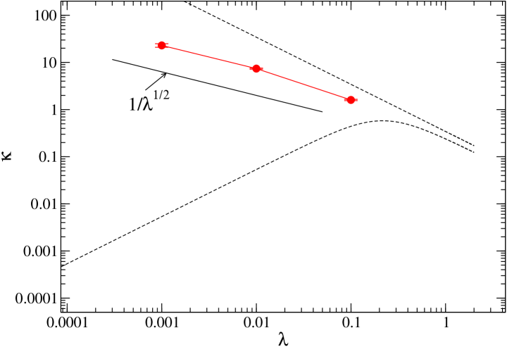
This corresponds to the case with $k_{o}>0$ and here we also set $k^{\prime}=1$. All results in this section were obtained by numerical solution of Eqs. (18). In Fig. (1) we plot $\langle J_{N}\rangle N/\Delta T$ versus $N$ for different values of the flipping rate $\lambda$ and with $\Delta=0.8,~{}k_{o}=4$. In all cases we see a rapid convergence to a system-size independent value which then gives the conductivity $\kappa$ of the system. In Fig. (2) we plot $\kappa$, obtained from the large-$N$ data in Fig. (1), as a function of $\lambda$. For comparison we also plot the lower and upper bounds for the Green-Kubo conductivity given by Eqs. (28,30). It is seen that $\kappa$ has a maximum around $\lambda\simeq 0.5$. This can be thought of as a balance between the flips delocalizing the phonons and acting as scatterers of phonons.

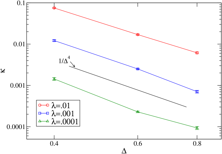
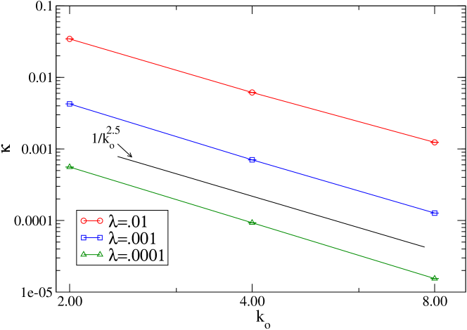
In accord with the bounds we find that at large $\lambda$, $\kappa\sim 1/\lambda$ while at small $\lambda$, the numerical results suggest $\kappa\sim\lambda$. We note that for $\lambda=0$, all phonon modes are exponentially localized within length-scales $\ell\sim(k_{o}\Delta^{2})^{-1}$. One can argue that for small values of $\lambda$ there is diffusion of energy between these localized states with a diffusion constant $\sim\ell^{2}\lambda$. This leads to the $\kappa\sim(k_{o}^{2}\Delta^{4})^{-1}\lambda$ and we now test this numerically. In Figs. (3,4) we show the numerical data which suggests the scalings $\kappa\sim\Delta^{-4}$ and $\kappa\sim{k_{o}}^{-2.5}$, which are roughly consistent with the expected behavior. The reason for the discrepancy could be that we are not yet in the strong localization regime where the prediction is expected to be most accurate.

Figure 1: (Color online)Plot of $JN/(T_{L}-T_{R})$ versus $N$ for for different values of $\lambda$. The parameter values were set at $k_{o}=4,k=1,\Delta=0.8$. All the data shown here were obtained from exact numerical computation.

Figure 2: (Color online) Plot of $\kappa$ versus $\lambda$ obtained from the numerical data in Fig. (1). The lower and upper bounds for $\kappa_{GK}$ given by Eqs. (28,30) are shown by the dashed lines.

Figure 3: (Color online)Plot of $\kappa$ versus $\Delta$ for different values of $\lambda$ and with $k_{o}=4$ and $k=1$. We also show a straight line with slope $-4.0$.

Figure 4: (Color Online)Plot of $\kappa$ versus $k_{o}$ for different values of $\lambda$ and with $\Delta=0.8$ and $k=1$. We also show a straight line with slope $-2.5$.

Figure 5: (Color Online)Plot of $JN/(T_{L}-T_{R})$ versus $N$ for the unpinned case with both fixed (dashed lines) and free BCs (solid lines) for different values of $\lambda$ and parameter values $k=1$ and $\Delta=0.8$. The data for $N<512$ were obtained using exact numerics and in all these cases simulations give very good agreement with the numerics. For $N\geq 512$, the data were obtained from simulations alone.

Figure 6: (Color Online)Plot of $\kappa$ versus $\lambda$ for the unpinned system obtained from the numerical data in Fig. (5). The lower and upper bounds for $\kappa_{GK}$ given by Eqs. (28,30) are shown by the dashed lines. Also shown is a straight line with slope $-1/2$.

Figure 7: (Color Online)Plot of temperature profile ($T_{i}=\langle p_{i}^{2}/m_{i}\rangle$) for the unpinned case (with mass disorder $\Delta=0.8$) with fixed BCs for $N=128,\lambda=5,T_{L}=4,T_{R}=1$. The expected linear profile is also shown. The data was obtained from exact numerical computation.

Figure 8: Same parameters as Fig. 7 except the velocity flip $\lambda\rightarrow 0$. The data shown is from an exact numerical computation with $\lambda=10^{-9}$. We have verified that this is close to the temperature profile for $\lambda=10^{-7}$ and expect that it is converging to the $\lambda=0$ value.

IV.2 Unpinned case

As noted above for the unpinned case with $\lambda=0$, the two different boundary conditions(BC) namely fixed BCs with $k^{\prime}>0$ and free BCs with $k^{\prime}=0$ give respectively $\langle J_{N}\rangle\sim N^{-3/2}$ casher71 and $\langle J_{N}\rangle\sim N^{-1/2}$ rubin71 . The difference in the asymptotic behavior of the current for different BCs can be understood as arising from the dependence on BCs of the transmission of the low frequency modes which carry the current dhar01 . For any $\lambda>0$ however we expect that the system should have a unique finite value of the conductivity, independent of boundary conditions, the same as for $\kappa_{GK}$. Physically we can argue as follows: The unpinned system without disorder has a finite positive $\kappa$ given by Eq. (24), which is independent of BCs [see comments at end of sec. (III.1)]. The low frequency modes are weakly affected by disorder hence we expect that as far as these modes are concerned the unpinned system with and without disorder will behave similarly. Since these are the modes which led to the dependence on BCs for the case $\lambda=0$, we expect that for $\lambda>0$ they will not have any effect.

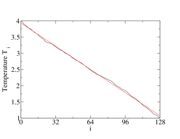
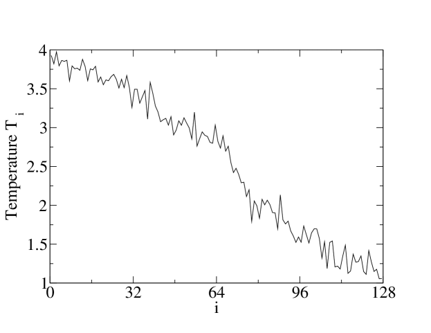
We now present results of our numerical and simulational studies of the unpinned chain with free and fixed BCs. The numerical results are obtained by solving Eqs. (18). The simulation involves evolving the system with the Hamiltonian part, the momentum flips at all sites and the Langevin baths at the boundary sites. For $N\leq 512$, the numerical method was employed to arrive at the solution for the NESS whereas for larger values of $N$, we performed simulations to obtain the data. In Fig. (5) we plot $JN/(T_{L}-T_{R})$ versus $N$ for different values of $\lambda$ for both fixed and free BCs. The disorder strength is $\Delta=0.8$. For both BCs we can see flattening of the curves at large system sizes for the parameter values $\lambda=0.1,0.01$ implying a finite $\kappa$, which is independent of BCs. For $\lambda=0.001,0.0001$ it appears that reaching the asymptotic limit requires larger system sizes. Using the large-$N$ data in Fig. (5) we estimate the conductivity $\kappa=JN/\Delta T$ and this is plotted in Fig. (6). In Fig. (7) we show a typical plot of the temperature profile for the case with fixed BC (this was obtained using exact numerics). The profile is close to linear consistent with the fact that the conductivity is temperature-independent. We do not see any significant boundary temperature jumps since the system size is sufficiently large. In Fig (8) we have the profile for N=128 for the case $\lambda\to 0$ which shows considerable jump in the temperatures across neighboring sites.

Table 1: Values of Correlation Functions for n=4 ($T_{L}=4,T_{R}=1$)

Correlation	$\lambda=0.1$	$\lambda=2$	$\lambda=10$
$\frac{<p_{1}^{4}>-3<p_{1}^{2}>^{2}}{<p_{1}^{2}>^{2}}$	0.006	0.014	$\sim 10^{-4}$
$\frac{<p_{2}^{4}>-3<p_{2}^{2}>^{2}}{<p_{2}^{2}>^{2}}$	0.054	0.058	0.049
$\frac{<p_{3}^{4}>-3<p_{3}^{2}>^{2}}{<p_{3}^{2}>^{2}}$	0.061	0.110	0.098
$\frac{<p_{4}^{4}>-3<p_{4}^{2}>^{2}}{<p_{4}^{2}>^{2}}$	0.038	0.018	0.002
$\frac{<p_{1}^{2}q_{1}^{2}>-<q_{1}^{2}><p_{1}^{2}>}{<q_{1}^{2}><p_{1}^{2}>}$	0.002	0.004	$\sim 10^{-5}$
$\frac{<p_{2}^{2}q_{2}^{2}>-<q_{2}^{2}><p_{2}^{2}>}{<q_{2}^{2}><p_{2}^{2}>}$	0.011	0.014	0.013
$\frac{<p_{3}^{2}q_{3}^{2}>-<q_{3}^{2}><p_{3}^{2}>}{<q_{3}^{2}><p_{3}^{2}>}$	0.012	0.025	0.023
$\frac{<p_{4}^{2}q_{4}^{2}>-<q_{4}^{2}><p_{4}^{2}>}{<q_{4}^{2}><p_{4}^{2}>}$	0.012	0.034	$\sim 10^{-4}$

It appears likely that for all $\lambda>0$ the conductivity $\kappa$ is independent of BCs. However this is difficult to verify from simulations since one needs to study very large system sizes to reach the correct asymptotic limit. The reason for this can be roughly seen as follows. In the ordered case the conductivity $\kappa\sim 1/\lambda$ and this can be understood in terms of an effective mean free path $\ell\sim 1/\lambda$ for the ballistic phonons because of scattering from the stochastic process. Hence we can expect that, to see diffusive behavior for the low frequency ballistic modes, important in the disordered case, requires one to study sizes $N\stackrel{{\scriptstyle>}}{{\sim}}\ell$ or $N\stackrel{{\scriptstyle>}}{{\sim}}1/\lambda$. Finally we observe from Fig. (6) that at small $\lambda$, the conductivity appears to be diverging as $1/\lambda^{1/2}$. In the absence of noise the localization length $\ell_{L}\sim 1/\omega^{2}$, hence it is expected that all modes with $\ell_{L}<\ell$ or $\omega>\lambda^{1/2}$ stay localized. The low frequency modes $0<\omega<\lambda^{1/2}$ become diffusive with mean free paths $\sim 1/\lambda$ thus resulting in a conductivity $\kappa\sim\lambda^{1/2}(1/\lambda)\sim 1/\lambda^{1/2}$, which explains the observed behavior.

V Discussion

We have shown here that the stationary one-body and pair correlations in the velocity flip model are the same (after setting $\gamma^{\prime}_{l}=2\lambda m_{l}$) as in the harmonic chain with self-consistent reservoirs. We have also numerically investigated the dependence of the thermal conductivity $\kappa$ of the disordered harmonic chain on the velocity flip rate $\lambda$. For $\lambda\to 0$ our results suggest $\kappa\sim\lambda$ for the pinned system and $\kappa\sim\lambda^{-1/2}$ for the unpinned system. Establishing these results conclusively requires further work.

We note that while for the self-consistent reservoirs model the NESS is exactly Gaussian, this is not so for our noisy model. Instead it will be in general a superposition of Gaussians. Computer simulations however indicate that the single particle distributions are very close to a single Gaussian while the joint distribution of $x_{l}$ and $p_{l}$ or of $p_{l}$ and $p_{j}$ , $j\neq l$, are essentially uncorrelated. In addition, the set of equations for the four variable correlation functions was derived and for small values of n, they were solved numerically. The exact values obtained from these numerics were found to be in close match with the simulation results. For n=4, and $T_{L}=4,T_{R}=1$, the results from the numerical solution are shown in table I corresponding to 3 different values of $\lambda$. It was also observed that these normalized forms of correlations (that go to zero when the temperatures of the two reservoirs are equal or when there is no velocity flipping) have a limit when either the difference in temperature ($T_{L}-T_{R}$) or strength of stochastic noise ($\lambda$) goes to infinity. When we let $\lambda\to\infty$, we observed that the correlations involving p1 and p4 went to zero.

We are currently investigating the $O(N)$ corrections to the pair correlations in the noisy NESS . These are known to behave like $1/N$ for certain diffusive lattice systems and to contribute terms of $O(N)$ beyond those obtained from the local equilibrium to the variance of the particle number in the NESS. Results of this kind are also known partially for the continuum case with a different kind of noise, i.e instead of velocity reversals pairs of nearest neighbor particles diffuse on the circle $p_{i}^{2}+p_{i+1}^{2}=C$.

VI Acknowledgements

We thank Cedric Bernardin, David Huse, Jani Lukkarinen and Stefano Olla for very helpful discussions. Joel Lebowitz and Venkateshan K were supported by NSF grant DMR 08-02120 and by AFOSR[grant AF-FA09550-07]. Joel Lebowitz also thanks the IHES and IHP for their hospitality during part of this work.

References

- (1) A. Dhar, Heat conduction in the disordered harmonic chain revisited, Phys. Rev. Lett. 86, 5882 (2001).
- (2) A. Dhar and J.L. Lebowitz, Effect of phonon-phonon interactions on localization, Phys. Rev. Lett. 100, 134301 (2008).
- (3) A. Casher and J. L. Lebowitz, Heat flow in regular and disordered harmonic chains, J. Math. Phys. 12, 1701 (1971.)
- (4) R. J. Rubin and W. L. Greer, Abnormal lattice thermal conductivity of a one dimensional, harmonic, isotopically disordered crystal, J. Math. Phys. 12, 1686 (1971).
- (5) C.Bernardin, Thermal Conductivity for a Noisy Disordered Harmonic Chain , J. Stat. Phys. 133, 417 (2008).
- (6) D. M. Basko, I. L. Aleiner, B. L. Altshuler On the problem of many-body localization, in A. L. Ivanov, S.- G. Tikhodeev (eds.), Problems of condensed matter physics, (Oxford University Press, NY, 2008), pp. 50-69.
- (7) V. Oganesyan, D. A. Huse, Localization of interacting fermions at high temperature, Phys. Rev. B 75, 155111 (2007).
- (8) A. S. Pikovsky and D.L.Shepelyansky,Destruction of Anderson localization by a weak nonlinearity, Phys. Rev. Lett. 100, 094101 (2008).
- (9) G. Kopidakis, S. Komineas, S. Flach, S. Aubry, Absence of wavepacket diffusion in disordered nonlinear systems , Phys. Rev. Lett. 100, 084103 (2008).
- (10) A. Dhar and K. Saito, Heat conduction in the disordered Fermi-Pasta-Ulam chain, Phys. Rev. E 78, 061136 (2008).
- (11) M. Mulansky, K. Ahnert, A. Pikovsky, D. L. Shepelyansky, Dynamical Thermalization of Disordered Nonlinear Lattices, Phys. Rev. E 80, 056212 (2009).
- (12) V. Oganesyan, A. Pal and D. A. Huse, Energy transport in disordered classical spin chains, Phys. Rev. B 80, 115104 (2009).
- (13) D. M. Basko, Weak chaos in the disordered nonlinear Schroedinger chain: destruction of Anderson localization by Arnold diffusion, arXiv:1005.5033 (2010).
- (14) L. Delfini, S. Lepri, R. Livi, and A. Politi, Nonequilibrium Invariant Measure under Heat Flow, Phys. Rev. Lett. 101, 120604 (2008).
- (15) S. Lepri, C Mejia-Monasterio and A. Politi, A stochastic model of anomalous heat transport: analytical solution of the steady state, J.Phys.A: Math. Theor. 42, 025001 (2009).
- (16) M. Bolsterli, M. Rich, and W. M. Visscher, Simulation of nonharmonic interactions in a crystal by self-consistent reservoirs, Phys. Rev. A 4, 1086 (1970).
- (17) M. Rich and W. M. Visscher, Disordered harmonic chain with self-consistent reservoirs, Phys. Rev. B 11, 2164 (1975).
- (18) F. Bonetto, J. L. Lebowitz, and J. Lukkarinen, Fourier’s law for a harmonic crystal with self-consistent reservoirs, J. Stat. Phys. 116, 783 (2004).
- (19) O. Ajanki and F. Huveneers, Rigorous scaling law for the heat current in disordered harmonic chain, arXiv:1003.1076.
- (20) T. Verheggen, Transmission coefficient and heat conduction of a harmonic chain with random masses: asymptotic estimates on products of random matrices, Commun. Math. Phys., 69-82 (1979).
- (21) C. Bernardin and S. Olla Fourier’s Law for a microscopic heat conduction model, Journal Of Statistical Physics 121 271-289 (2005).
- (22) S. Sethuraman Central Limit Thorem for additive functionals of the simple exclusion process, The Annals of Probability 28, 277-302 (2000).