Soft-Gluon Resummation and the Valence Parton Distribution Function of the Pion
Abstract
We determine the valence parton distribution function of the pion by performing a new analysis of data for the Drell-Yan process . Compared to previous analyses, we include next-to-leading-logarithmic threshold resummation effects in the calculation of the Drell-Yan cross section. As a result of these, we find a considerably softer valence distribution at high momentum fractions than obtained in previous next-to-leading-order analyses, in line with expectations based on perturbative-QCD counting rules or Dyson-Schwinger equations.
pacs:
12.38.Cy,12.38.Bx,14.40.BeAlthough the pion is one of the most important particles in strong-interaction physics, our knowledge about its internal quark and gluon “partonic” structure is still rather poor. Most of the available information comes from Drell-Yan dimuon production by charged pions incident on nuclear fixed targets Conway:1989fs ; Bordalo:1987cr ; DYreview . These data primarily constrain the valence distribution . Several next-to-leading order (NLO) analyses of the Drell-Yan data have been performed Sutton:1991ay ; Gluck:1999xe ; Wijesooriya:2005ir . A striking feature has been that the resulting valence distribution turned out to be rather hard at high momentum fraction , typically showing only a linear or slightly faster falloff. This finding is at variance with predictions based on perturbative QCD Farrar:1979aw , and calculations using Dyson-Schwinger equations Hecht:2000xa , for which the falloff is expected to be . On the other hand, Nambu-Jona-Lasinio Shigetani:1993dx and constituent quark models Frederico:1994dx , as well as duality arguments Melnitchouk:2002gh , favor a linear behavior. The high- behavior of is widely regarded to be an important so-far-unresolved problem in strong-interaction physics Holt:2010vj .
In the kinematic regimes accessed by the fixed-target Drell-Yan data, perturbative corrections beyond NLO may be significant Shimizu:2005fp . The relation sets a threshold for the partonic reaction, where and denote the invariant mass of the lepton pair and the overall hadronic center-of-mass (c.m.) energy, respectively, and and are the momentum fractions of the partons participating in the hard-scattering reaction. As increases toward unity, little phase space for real-gluon radiation remains, since most of the initial partonic energy is used to produce the virtual photon. The infrared cancellations between virtual and real-emission diagrams then leave behind large logarithmic higher-order corrections to the cross sections, the so-called threshold logarithms. These logarithms become particularly important in the fixed-target regime, because here the ratio is relatively large. It then becomes necessary to resum the large corrections to all orders in the strong coupling, a technique known as threshold resummation. QCD threshold resummation for the Drell-Yan process has been derived a long time ago Sterman:1986aj . It turns out that the threshold logarithms lead to a strong increase of the cross section near threshold. Therefore, if threshold resummation effects are included, it is possible that a much softer valence distribution of the pion is sufficient to describe the experimental data. Indeed, as was observed in Ref. Wijesooriya:2005ir , the extracted already becomes softer when going from the lowest order to NLO, where the threshold logarithms first appear. In this Letter, we will address the impact of resummation effects on the pion’s valence distribution. We will find that indeed a falloff even at a relatively low resolution scale is well consistent with the Drell-Yan data. We note that the effects of resummation on parton distributions were also examined in the context of deep-inelastic lepton scattering Corcella:2005us .
We consider the inclusive cross section for the production of a pair of invariant mass and rapidity in the process , where denotes a nucleon or nuclear target and and are the four-momenta of the initial-state particles. According to the factorization theorem, the cross section is written as
| (1) | |||||
where , with , and where
| (2) |
with . At lowest order, one has . The sum in Eq. (1) runs over all partonic channels, with and the corresponding parton distribution functions of the pion and the nucleus and the hard-scattering function. The latter can be computed in perturbation theory as a series in the strong coupling constant , starting from the lowest-order process . The functions in (1) depend on the factorization and renormalization scales, which we choose to be equal here and collectively denote as .
As discussed above, our goal is to resum large logarithmic contributions to that arise near partonic threshold , where , with the partonic c.m. energy. Resummation may be achieved in Mellin moment space, where phase space integrals for multiple-soft-gluon emission decouple. For the rapidity-dependent cross section, it is convenient to also apply a Fourier transform in Sterman:2000pt ; Mukherjee:2006uu . Under combined Fourier and Mellin transforms of the cross section,
| (3) |
the convolution integrals in (1) decouple into ordinary products Mukherjee:2006uu ; Sterman:2000pt . Defining the moments of the parton distribution functions,
| (4) |
and introducing the corresponding double transform of the partonic hard-scattering cross sections,
| (5) |
where is the partonic c.m. rapidity, one finds
| (6) |
As was discussed in Refs. Laenen:1992ey ; Mukherjee:2006uu ; Bolzoni:2006ky , in the near-threshold limit or , the dependence of on becomes subleading and may be neglected. The resummed expression for then becomes identical to that for the total (rapidity-integrated) Drell-Yan cross section and is given in the scheme by
| (7) | |||||
where is a perturbative function, whose first two orders are sufficient for resummation to next-to-leading-logarithmic (NLL) order Sterman:1986aj :
| (8) |
with Kodaira:1981nh
| (9) |
Here and . The first term in Eq. (7) does not originate from soft-gluon emission but instead mostly contains hard virtual corrections. It is also a perturbative series in , and we need only its first-order term:
| (10) |
whose exponentiated form is given in Ref. Eynck:2003fn . As was shown in Ref. Mukherjee:2006uu , rapidity dependence is slightly more faithfully reproduced if one shifts the Mellin moments to in , which is a choice that we also adopt here.
At NLL order, the expression in Eq. (7) becomes Catani:1996yz
| (11) |
where with the Euler constant , and
| (12) |
The functions and collect all leading-logarithmic and NLL terms in the exponent, which are of the form and , respectively. They read
where
| (14) | |||||
| (15) |
The resummed hadronic rapidity-dependent cross section is obtained by taking the inverse Mellin and Fourier transforms of Eq. (6):
| (16) |
When performing the inverse Mellin transform, the parameter usually has to be chosen in such a way that all singularities of the integrand lie to the left of the integration contour. The resummed cross section has a Landau singularity at or , as a result of the divergence of the running coupling in (7) for . In the Mellin inversion, we adopt the minimal prescription developed in Ref. Catani:1996yz to deal with the Landau pole, for which the contour is chosen to lie to the left of the Landau singularity. An alternative possibility is to perform the resummation directly in -space Becher:2007ty . We match the resummed cross section to the NLO one by subtracting the expansion of the resummed expression and adding the full NLO cross section Mukherjee:2006uu .
The fixed-target pion Drell-Yan data Conway:1989fs ; Bordalo:1987cr are in a kinematic regime where the partons’ momentum fractions are relatively large, (), and hence the valence quark contributions strongly dominate. We can therefore only hope to determine the pion’s valence distribution . Following the NLO Glück-Reya-Schienbein (GRS) analysis Gluck:1999xe , we choose the initial scale for the evolution and parameterize the valence distribution function as
| (17) |
subject to the constraint . Since there is no sensitivity to the sea quark and gluon distributions, we adopt them from the GRS analysis, except that we modify the overall normalization of the sea quark distribution so that the momentum sum rule is maintained when we determine the valence distribution. All distributions are then evolved at NLO to the relevant factorization scale .
| Fit | (no. of points) | |||||
|---|---|---|---|---|---|---|
| 1 | 0.55 | |||||
| 2 | 0.60 | |||||
| 3 | 0.65 | |||||
| 4 | 0.7 |
The free parameters in Eq. (17) are determined by a fit to the pion Drell-Yan data from the Fermilab E615 experiment Conway:1989fs , applying threshold resummation as detailed in the previous section. The E615 data were obtained by using a 252 GeV beam on a tungsten target. We take into account the nuclear effects in this heavy target by using the nuclear parton distribution functions from Ref. deFlorian:2003qf . We use data points with lepton pair mass 4.03 GeV 8.53 GeV (between the and resonances) and . Here, is the Feynman variable. In the near-threshold region, which is addressed by threshold resummation, we can use lowest-order kinematics to determine the relation between and the rapidity :
| (18) |
Since the E615 data have a nominal overall systematic error of , we introduce a normalization factor that multiplies the theoretical cross section. We find that the parameter in (17) is not well-determined, and we hence fix it to , a value roughly preferred by the fit. In order to obtain a better picture of the physical content of our determined pion valence distribution, we perform fits for several different values of its total momentum fraction . Fixing makes one parameter in Eq. (17) redundant, which we choose to be . We hence fit the remaining three free parameters , and to the 70 data points using a minimization procedure.
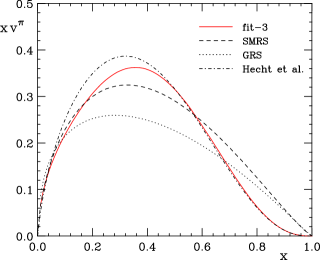
The results are shown in Table 1, for four different values of the total valence quark momentum fraction . One observes that fit 3 for which the valence carries of the pion’s momentum is preferred, with slightly higher or lower values also well acceptable. Most importantly, all fits show a clear preference for a falloff much softer than linear, with fits 2, 3, and 4 having a value of very close to . This is the central result of our work. The valence distribution for our best fit 3 is shown in Fig. 1, evolved to . At this scale it behaves as . Valence distributions obtained from previous NLO analyses Sutton:1991ay ; Gluck:1999xe , which have a roughly linear behavior at high , and from calculations using Dyson-Schwinger equations Hecht:2000xa , for which , are also shown. We note that for all our fits the factors lie well within the normalization uncertainty of the data.


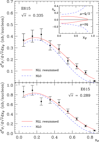
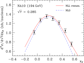
In Fig. 2 we compare the resummed Drell-Yan cross section obtained for fit 3 to some of the E615 data. We have chosen the factorization and renormalization scale . As one can see from the figure and from Table 1, the data are very well described. This also holds true for the CERN NA10 Bordalo:1987cr Drell-Yan data, which were not included in our fit, and to which we compare in Fig. 3. We also show the results obtained for our fit 3 when using only NLO (i.e., unresummed) partonic cross sections in the calculation. As seen in Fig. 2, these fall off too rapidly at large . The inset in Fig. 2 shows the variation of our NLO and resummed cross sections with , in terms of the quantity , with , . As one can see, the scale uncertainty is significantly reduced after resummation and becomes smaller than the experimental uncertainties, in particular in the region of high . This implies that our findings for the pion’s valence distribution are stable with respect to the main theoretical uncertainty in the calculation.
In conclusion, we have determined a new valence parton distribution function for the pion by reanalyzing pion-nucleon Drell-Yan data including threshold-resummed contributions to the cross section. The obtained valence distribution is much softer in the high- regime than that found in an NLO analysis, behaving roughly as , in agreement with predictions from perturbative QCD and nonperturbative Dyson-Schwinger equation approaches.
We are grateful to F. Yuan for useful communications. This work was supported by BMBF. M.A. was supported by a grant of the “Bayerische Eliteförderung.” W.V.’s work has been supported by the U.S. Department of Energy (Contract No. DE-AC02-98CH10886) and by the Alexander von Humboldt Foundation.

References
- (1) J. S. Conway et al. [E615 Collaboration], Phys. Rev. D 39, 92 (1989).
- (2) P. Bordalo et al. [NA10 Collaboration], Phys. Lett. B 193, 373 (1987); B. Betev et al. [NA10 Collaboration], Z. Phys. C 28, 9 (1985).
- (3) For a review, see: W. J. Stirling and M. R. Whalley, J. Phys. G 19, D1 (1993).
- (4) P. J. Sutton et al., Phys. Rev. D 45, 2349 (1992).
- (5) M. Glück, E. Reya and I. Schienbein, Eur. Phys. J. C 10, 313 (1999).
- (6) K. Wijesooriya, P. E. Reimer and R. J. Holt, Phys. Rev. C 72, 065203 (2005).
- (7) G. R. Farrar and D. R. Jackson, Phys. Rev. Lett. 43, 246 (1979); E. L. Berger and S. J. Brodsky, Phys. Rev. Lett. 42, 940 (1979); S. J. Brodsky and F. Yuan, Phys. Rev. D 74, 094018 (2006); F. Yuan, Phys. Rev. D 69, 051501 (2004).
- (8) M. B. Hecht, C. D. Roberts and S. M. Schmidt, Phys. Rev. C 63, 025213 (2001).
- (9) T. Shigetani, K. Suzuki and H. Toki, Phys. Lett. B 308, 383 (1993).
- (10) T. Frederico and G. A. Miller, Phys. Rev. D 50, 210 (1994); A. Szczepaniak, C. R. Ji and S. R. Cotanch, Phys. Rev. D 49, 3466 (1994).
- (11) W. Melnitchouk, Eur. Phys. J. A 17, 223 (2003).
- (12) R. J. Holt and C. D. Roberts, Rev. Mod. Phys. 82, 2991 (2010).
- (13) H. Shimizu et al., Phys. Rev. D 71, 114007 (2005).
- (14) G. F. Sterman, Nucl. Phys. B 281, 310 (1987); S. Catani and L. Trentadue, Nucl. Phys. B 327, 323 (1989).
- (15) G. Corcella and L. Magnea, Phys. Rev. D 72, 074017 (2005).
- (16) G. F. Sterman and W. Vogelsang, JHEP 0102, 016 (2001).
- (17) A. Mukherjee and W. Vogelsang, Phys. Rev. D 73, 074005 (2006).
- (18) E. Laenen and G. Sterman, FERMILAB Report No. CONF-92-359-T (unpublished).
- (19) P. Bolzoni, Phys. Lett. B 643, 325 (2006).
- (20) J. Kodaira and L. Trentadue, Phys. Lett. B 112, 66 (1982).
- (21) T. O. Eynck, E. Laenen and L. Magnea, JHEP 0306, 057 (2003).
- (22) S. Catani et al., Nucl. Phys. B 478, 273 (1996).
- (23) T. Becher, M. Neubert and G. Xu, JHEP 0807, 030 (2008).
- (24) D. de Florian and R. Sassot, Phys. Rev. D 69, 074028 (2004).