Enumeration of \CH\C𝐻\C{H}-strata in quantum matrices with respect to dimension

J. Bell, K. Casteels and S. Launois Jason Bell
Department of Mathematics
Simon Fraser University
Burnaby, BC V5A 1S6, Canada
jpb@math.sfu.ca Karel Casteels
Department of Mathematics
University of California
Santa Barbara, CA 93106
casteels@math.ucsb.edu Stéphane Launois
School of Mathematics, Statistics & Actuarial science
University of Kent
Canterbury, Kent CT2 7NF, United Kingdom
S.Launois@kent.ac.uk
Abstract.

We present a combinatorial method to determine the dimension of \CH\C𝐻\C{H}-strata in the algebra of m×n𝑚𝑛m\times n quantum matrices 𝒪q(Mm,n(𝕂))subscript𝒪𝑞subscript𝑀𝑚𝑛𝕂\mathcal{O}_{q}(M_{m,n}(\mathbb{K})) as follows. To a given \CH\C𝐻\C{H}-stratum we associate a certain permutation via the notion of pipe-dreams. We show that the dimension of the \CH\C𝐻\C{H}-stratum is precisely the number of odd cycles in this permutation. Using this result, we are able to give closed formulas for the trivariate generating function that counts the d𝑑d-dimensional \CH\C𝐻\C{H}-strata in 𝒪q(Mm,n(𝕂))subscript𝒪𝑞subscript𝑀𝑚𝑛𝕂\mathcal{O}_{q}(M_{m,n}(\mathbb{K})). Finally, we extract the coefficients of this generating function in order to settle conjectures proposed by the first and third named authors [3, 4] regarding the asymptotic proportion of d𝑑d-dimensional \CH\C𝐻\C{H}-strata in 𝒪q(Mm,n(𝕂))subscript𝒪𝑞subscript𝑀𝑚𝑛𝕂\mathcal{O}_{q}(M_{m,n}(\mathbb{K})).

2000 Mathematics Subject Classification:
16W35; 20G42
The first and second named authors thank NSERC for its generous support. The third named author’s research was supported by a Marie Curie European Reintegration Grant within the 7thsuperscript7th7^{\mbox{th}} European Community Framework Programme

1. Introduction

For positive integers m𝑚m and n𝑛n and for q𝑞q a nonzero element of a field 𝕂𝕂\mathbb{K} that is not a root of unity, let us denote by \CA=𝒪q(Mm,n(𝕂))\C𝐴subscript𝒪𝑞subscript𝑀𝑚𝑛𝕂\C{A}=\mathcal{O}_{q}(M_{m,n}(\mathbb{K})) the algebra of m×n𝑚𝑛m\times n quantum matrices. There is a natural action of the algebraic torus \CH=(𝕂)m+n\C𝐻superscriptsuperscript𝕂𝑚𝑛\C{H}=(\mathbb{K}^{*})^{m+n} on \CA\C𝐴\C{A} which, by work of Goodearl and Letzter [6] allows the prime spectrum of \CA\C𝐴\C{A} to be partitioned into a finite number of disjoint \CH\C𝐻\C{H}-strata. Moreover, each \CH\C𝐻\C{H}-stratum is homeomorphic (with respect to the Zariski topology) to the prime spectrum of a commutative Laurent polynomial ring over 𝕂𝕂\mathbb{K}.

In this work, we complete the project started in [5] and continued in [3, 4]; namely, that of determining a useful condition to determine the dimension of a given \CH\C𝐻\C{H}-stratum. Furthermore, this condition enables one to easily enumerate the \CH\C𝐻\C{H}-strata in 𝒪q(Mm,n(𝕂))subscript𝒪𝑞subscript𝑀𝑚𝑛𝕂\mathcal{O}_{q}(M_{m,n}(\mathbb{K})) with respect to dimension. The principal motivation for this originates in Dixmier’s idea that for an infinite-dimensional algebra, identifying the primitive ideals forms an important first step towards understanding the representation theory of the algebra. On the other hand, as a consequence of the \CH\C𝐻\C{H}-stratification theory, the primitive ideals are those prime ideals that are maximal within their \CH\C𝐻\C{H}-stratum. In particular, primitive \CH\C𝐻\C{H}-primes correspond to zero-dimensional \CH\C𝐻\C{H}-strata.

Our condition is roughly described as follows. Within each \CH\C𝐻\C{H}-stratum there is a unique prime ideal that is invariant under the action of \CH\C𝐻\C{H}, a so-called \CH\C𝐻\C{H}-prime. Next, to any given \CH\C𝐻\C{H}-prime, we may associate a certain permutation τ𝜏\tau, which for reasons that will become clear, we call a toric permutation. Our first main result is the following theorem.

Theorem 1.1.

Let J𝐽J be an \CH\C𝐻\C{H}-prime in 𝒪q(Mm,n(𝕂))subscript𝒪𝑞subscript𝑀𝑚𝑛𝕂\mathcal{O}_{q}(M_{m,n}(\mathbb{K})) and let τ𝜏\tau be the associated toric permutation. The dimension of the \CH\C𝐻\C{H}-stratum containing J𝐽J is precisely the number of odd cycles in the disjoint cycle decomposition of τ𝜏\tau.

To clarify, the parity of a cycle is defined to be the parity of the number of inversions. Thus a cycle is odd if and only if it has even length.

The crucial point in the proof of Theorem 1.1 is an isomorphism given in Theorem 4.6 between the kernels of certain linear maps. Before describing this, we note that the authors [2], and independently Yakimov [19] with stronger hypotheses on 𝕂𝕂\mathbb{K} and q𝑞q, have generalized the isomorphism to obtain a formula for calculating the dimension of torus-invariant strata in certain important subalgebras of the quantized enveloping algebra Uq(𝔤)subscript𝑈𝑞𝔤U_{q}(\mathfrak{g}) of a simple complex Lie algebra 𝔤𝔤\mathfrak{g}. In this work we give a proof in the context of quantum matrices both for completeness and for its interesting combinatorial nature.

The proof of Theorem 1.1 depends on two parametrizations of the set of \CH\C𝐻\C{H}-primes of 𝒪q(Mm,n(𝕂))subscript𝒪𝑞subscript𝑀𝑚𝑛𝕂\mathcal{O}_{q}(M_{m,n}(\mathbb{K})). The first, due to Cauchon [7], assigns to every \CH\C𝐻\C{H}-prime a combinatorial object called a Cauchon diagram. This is simply an m×n𝑚𝑛m\times n grid of squares coloured black or white according to the rule that if a square is black, then either all squares strictly above or all squares strictly to the left are also black. See Figure 1 for some examples. Interestingly, Cauchon diagrams appear independently in the work of Postnikov [15] under the name L -diagrams (or “le”-diagrams), as a parametrization of the totally nonnegative Grassmann cells of the totally nonnegative Grassmannian. The connection between quantum matrices and total nonnegativity is detailed in papers of Goodearl, Launois and Lenagan [10, 9, 14].

The second parametrization of \CH\C𝐻\C{H}-primes consist of the set of restricted (m+n𝑚𝑛m+n)-permutations, that is, permutations σSm+n𝜎subscript𝑆𝑚𝑛\sigma\in S_{m+n} that satisfy

nσ(i)im𝑛𝜎𝑖𝑖𝑚-n\leq\sigma(i)-i\leq m

for all i{1,,m+n}𝑖1𝑚𝑛i\in\{1,\ldots,m+n\}. In [13] it has been shown that the set of restricted (m+n𝑚𝑛m+n)-permutations ordered under the reverse Bruhat order is order-isomorphic to the poset of \CH\C𝐻\C{H}-primes ordered by inclusion. This result was recently generalized by Yakimov [18]. A bijection between the set of Cauchon diagrams and the set of restricted permutations can be made using pipe dreams (see Section 3).

Bell and Launois [3] have shown that the dimension of a given \CH\C𝐻\C{H}-stratum may be computed using the associated Cauchon diagram D𝐷D. In particular, they show that one may construct a certain skew-symmetric matrix M(D)𝑀𝐷M(D) from D𝐷D such that the dimension of the \CH\C𝐻\C{H}-stratum is exactly dim(ker(M(D))\dim(\ker(M(D)).

We let ω𝜔\omega denote the maximum element in the poset of restricted (m+n)𝑚𝑛(m+n)-permutations, and suppose that we have a Cauchon diagram D𝐷D whose corresponding restricted permutation is σ𝜎\sigma. The toric permutation corresponding to D𝐷D is defined to be the permutation τ=σω1𝜏𝜎superscript𝜔1\tau=\sigma\omega^{-1}. In Theorem 4.6 we construct an isomorphism between ker(M(D))kernel𝑀𝐷\ker(M(D)) and ker(Pσ+Pω)kernelsubscript𝑃𝜎subscript𝑃𝜔\ker(P_{\sigma}+P_{\omega}), where Pμsubscript𝑃𝜇P_{\mu} is the matrix representation of a permutation μ𝜇\mu. As this latter space has dimension equal to the number of odd cycles of τ𝜏\tau, we obtain Theorem 1.1.

As an application we are able to show in Corollary 5.3 that the number of d𝑑d-dimensional \CH\C𝐻\C{H}-strata in 𝒪q(Mm,n(𝕂))subscript𝒪𝑞subscript𝑀𝑚𝑛𝕂\mathcal{O}_{q}(M_{m,n}(\mathbb{K})) is the coefficient of xmm!ynn!tdsuperscript𝑥𝑚𝑚superscript𝑦𝑛𝑛superscript𝑡𝑑\frac{x^{m}}{m!}\frac{y^{n}}{n!}{t^{d}} in the power series expansion of

(ey+ex1)1t2(ex+ey1)1t2.superscriptsuperscript𝑒𝑦superscript𝑒𝑥11𝑡2superscriptsuperscript𝑒𝑥superscript𝑒𝑦11𝑡2(e^{-y}+e^{-x}-1)^{\frac{-1-t}{2}}(e^{x}+e^{y}-1)^{\frac{1-t}{2}}.

By determining the coefficients of this power series, we are able to settle several conjectures from [4, 3] concerning the asymptotic proportion of d𝑑d-dimensional \CH\C𝐻\C{H}-strata in 𝒪q(Mm,n(𝕂))subscript𝒪𝑞subscript𝑀𝑚𝑛𝕂\mathcal{O}_{q}(M_{m,n}(\mathbb{K})). Namely, we prove in Theorem 5.6 that for fixed m𝑚m and d𝑑d, the proportion of d𝑑d-dimensional \CH\C𝐻\C{H}-strata in 𝒪q(Mm,n(𝕂))subscript𝒪𝑞subscript𝑀𝑚𝑛𝕂\mathcal{O}_{q}(M_{m,n}(\mathbb{K})) tends to a(d)m!2m𝑎𝑑𝑚superscript2𝑚\frac{a(d)}{m!2^{m}} as n𝑛n\rightarrow\infty, where a(d)𝑎𝑑a(d) is the coefficient of tdsuperscript𝑡𝑑t^{d} in the polynomial (t+1)(t+3)(t+2m1)𝑡1𝑡3𝑡2𝑚1(t+1)(t+3)\cdots(t+2m-1).

2. Preliminaries

In this section, we give some basic background on quantum matrices, the Goodearl-Letzter stratification theory, and Cauchon diagrams.

2.1. Quantum Matrices

Throughout this paper, we set 𝕂𝕂\mathbb{K} to be a field, q𝑞q is a nonzero element of 𝕂𝕂\mathbb{K} that is not a root of unity, and we fix two positive integers m𝑚m and n𝑛n. For a positive integer \ell, let []:={1,2,,}assigndelimited-[]12[\ell]:=\{1,2,\ldots,\ell\}.

Definition 2.1.

We let 𝒪q(Mm,n(𝕂))subscript𝒪𝑞subscript𝑀𝑚𝑛𝕂\mathcal{O}_{q}(M_{m,n}(\mathbb{K})) denote the quantized coordinate ring of m×n𝑚𝑛m\times n matrices. This is the algebra with generators xi,jsubscript𝑥𝑖𝑗x_{i,j} for all (i,j)[m]×[n]𝑖𝑗delimited-[]𝑚delimited-[]𝑛(i,j)\in[m]\times[n], subject to the following relations:

  1. (1)

    For all i[m]𝑖delimited-[]𝑚i\in[m] and j,k[n]𝑗𝑘delimited-[]𝑛j,k\in[n] with j<k𝑗𝑘j<k,

    xi,jxi,k=qxi,kxi,j;subscript𝑥𝑖𝑗subscript𝑥𝑖𝑘𝑞subscript𝑥𝑖𝑘subscript𝑥𝑖𝑗x_{i,j}x_{i,k}=qx_{i,k}x_{i,j};
  2. (2)

    For all j[n]𝑗delimited-[]𝑛j\in[n] and i,[m]𝑖delimited-[]𝑚i,\ell\in[m] with i<𝑖i<\ell,

    xi,jx,j=qx,jxi,j;subscript𝑥𝑖𝑗subscript𝑥𝑗𝑞subscript𝑥𝑗subscript𝑥𝑖𝑗x_{i,j}x_{\ell,j}=qx_{\ell,j}x_{i,j};
  3. (3)

    For all i,[m]𝑖delimited-[]𝑚i,\ell\in[m] with i<𝑖i<\ell and distinct j,k[n]𝑗𝑘delimited-[]𝑛j,k\in[n]:

    xi,jx,k={x,kxi,j, if j>k;x,kxi,j+(qq1)xi,kx,j, if j<k.subscript𝑥𝑖𝑗subscript𝑥𝑘casessubscript𝑥𝑘subscript𝑥𝑖𝑗 if j>k;subscript𝑥𝑘subscript𝑥𝑖𝑗𝑞superscript𝑞1subscript𝑥𝑖𝑘subscript𝑥𝑗 if j<k.x_{i,j}x_{\ell,k}=\left\{\begin{array}[]{ll}x_{\ell,k}x_{i,j},&\textnormal{ if $j>k$;}\\ x_{\ell,k}x_{i,j}+(q-q^{-1})x_{i,k}x_{\ell,j},&\textnormal{ if $j<k$.}\end{array}\right.

The algebra 𝒪q(Mm,n(𝕂))subscript𝒪𝑞subscript𝑀𝑚𝑛𝕂\mathcal{O}_{q}(M_{m,n}(\mathbb{K})) is colloquially known as the algebra of m×n𝑚𝑛m\times n quantum matrices, or just quantum matrices. It is well-known that 𝒪q(Mm,n(𝕂))subscript𝒪𝑞subscript𝑀𝑚𝑛𝕂\mathcal{O}_{q}(M_{m,n}(\mathbb{K})) may be presented as an iterated Ore extension of the base field. We set X𝑋X to be the matrix of generators obtained by setting X[i,j]:=xi,jassign𝑋𝑖𝑗subscript𝑥𝑖𝑗X[i,j]:=x_{i,j}. The collection of prime ideals of 𝒪q(Mm,n(𝕂))subscript𝒪𝑞subscript𝑀𝑚𝑛𝕂\mathcal{O}_{q}(M_{m,n}(\mathbb{K})) is the prime spectrum and is denoted by spec(𝒪q(Mm,n(𝕂)))specsubscript𝒪𝑞subscript𝑀𝑚𝑛𝕂{\rm spec}(\mathcal{O}_{q}(M_{m,n}(\mathbb{K}))). We endow the prime spectrum with the Zariski topology. As we assume that q𝑞q is not a root of unity, every prime ideal of 𝒪q(Mm,n(𝕂))subscript𝒪𝑞subscript𝑀𝑚𝑛𝕂\mathcal{O}_{q}(M_{m,n}(\mathbb{K})) is completely prime [11].

2.2. \CH\C𝐻\C{H}-Stratification Theory

We wish to understand the structure of spec(𝒪q(Mm,n(𝕂)))specsubscript𝒪𝑞subscript𝑀𝑚𝑛𝕂{\rm spec}(\mathcal{O}_{q}(M_{m,n}(\mathbb{K}))). To this end, a useful tool is the \CH\C𝐻\C{H}-stratification of Goodearl and Letzter. First notice that the algebraic torus \CH=(𝕂)m+n\C𝐻superscriptsuperscript𝕂𝑚𝑛\C{H}=(\mathbb{K}^{*})^{m+n} acts rationally by automorphisms on 𝒪q(Mm,n(𝕂))subscript𝒪𝑞subscript𝑀𝑚𝑛𝕂\mathcal{O}_{q}(M_{m,n}(\mathbb{K})) as follows. If

h=(ρ1,,ρm,γ1,,γn)\CH,subscript𝜌1subscript𝜌𝑚subscript𝛾1subscript𝛾𝑛\C𝐻h=(\rho_{1},\ldots,\rho_{m},\gamma_{1},\ldots,\gamma_{n})\in\C{H},

then for all (i,j)[m]×[n]𝑖𝑗delimited-[]𝑚delimited-[]𝑛(i,j)\in[m]\times[n] we set

hxi,j:=ρiγjxi,j.assignsubscript𝑥𝑖𝑗subscript𝜌𝑖subscript𝛾𝑗subscript𝑥𝑖𝑗h\cdot x_{i,j}:=\rho_{i}\gamma_{j}x_{i,j}.

An ideal J𝐽J is an \CH\C𝐻\C{H}-ideal if hJ=J𝐽𝐽h\cdot J=J for all h\CH\C𝐻h\in\C{H}. An \CH\C𝐻\C{H}-ideal P𝑃P is called an \CH\C𝐻\C{H}-prime ideal if, for any \CH\C𝐻\C{H}-ideals I𝐼I and J𝐽J, IJP𝐼𝐽𝑃IJ\subseteq P implies either IP𝐼𝑃I\subseteq P or JP𝐽𝑃J\subseteq P. It can be shown that an \CH\C𝐻\C{H}-prime ideal is, in fact, a prime ideal. The collection of all \CH\C𝐻\C{H}-prime ideals is denoted by -spec(𝒪q(Mm,n(𝕂)))-specsubscript𝒪𝑞subscript𝑀𝑚𝑛𝕂\mathcal{H}\textnormal{-spec}(\mathcal{O}_{q}(M_{m,n}(\mathbb{K}))).

Theorem 2.2 (Goodearl and Letzter [6]).

For the algebra \CA=𝒪q(Mm,n(𝕂))\C𝐴subscript𝒪𝑞subscript𝑀𝑚𝑛𝕂\C{A}=\mathcal{O}_{q}(M_{m,n}(\mathbb{K})), the following hold.

  1. (1)

    There are only finitely many \CH\C𝐻\C{H}-prime ideals.

  2. (2)

    The set spec(\CA\C𝐴\C{A}) can be partitioned into a disjoint union as follows:

    spec(\CA)=J-spec(\CA)YJ,spec\C𝐴subscript𝐽-spec\C𝐴subscript𝑌𝐽\emph{spec}(\C{A})=\bigcup_{J\in\mathcal{H}\text{\emph{-spec}}(\C{A})}Y_{J},

    where

    YJ:={Pspec(𝒜)hhP=J}assignsubscript𝑌𝐽conditional-set𝑃spec𝒜subscript𝑃𝐽\displaystyle{Y_{J}:=\{P\in\text{\emph{spec}}(\mathcal{A})\mid\bigcap_{h\in\mathcal{H}}h\cdot P=J\}}

    is the \CH\C𝐻\C{H}-stratum associated to J𝐽J.

  3. (3)

    Each \CH\C𝐻\C{H}-stratum is homeomorphic to the prime spectrum of a commutative Laurent polynomial ring over 𝕂𝕂\mathbb{K}.

  4. (4)

    The primitive ideals of spec(\CA)spec\C𝐴{\rm spec}(\C{A}) are precisely those ideals that are maximal within their \CH\C𝐻\C{H}-stratum.

The dimension of an \CH\C𝐻\C{H}-stratum YJsubscript𝑌𝐽Y_{J} is the Krull dimension of the commutative Laurent polynomial ring for which YJsubscript𝑌𝐽Y_{J} is homeomorphic to by Theorem 2.2(3). In other words, the dimension of YJsubscript𝑌𝐽Y_{J} is the length d𝑑d of the longest chain P0P1Pdsubscript𝑃0subscript𝑃1subscript𝑃𝑑P_{0}\subset P_{1}\subset\cdots\subset P_{d} of prime ideals contained in YJsubscript𝑌𝐽Y_{J}.

2.3. Cauchon Diagrams

The deleting-derivations algorithm due to Cauchon and applied to the algebra 𝒪q(Mm,n(𝕂))subscript𝒪𝑞subscript𝑀𝑚𝑛𝕂\mathcal{O}_{q}(M_{m,n}(\mathbb{K})) allows one to obtain a nice combinatorial parametrization of -spec(𝒪q(Mm,n(𝕂)))-specsubscript𝒪𝑞subscript𝑀𝑚𝑛𝕂\mathcal{H}\textnormal{-spec}(\mathcal{O}_{q}(M_{m,n}(\mathbb{K}))).

Definition 2.3.

An m×n𝑚𝑛m\times n diagram is simply an m×n𝑚𝑛m\times n grid of squares, each square coloured either white or black. A diagram is a Cauchon diagram if the colouring has the property that if a square is black, then either every square strictly above or every square strictly to the left is also black.

Refer to caption
Figure 1. Three 3×3333\times 3 diagrams. The left and center diagrams are Cauchon; the right diagram is not.
Theorem 2.4 (Cauchon [8]).

For every m𝑚m and n𝑛n, -spec(𝒪q(Mm,n(𝕂)))-specsubscript𝒪𝑞subscript𝑀𝑚𝑛𝕂\mathcal{H}\textnormal{-spec}(\mathcal{O}_{q}(M_{m,n}(\mathbb{K}))) is in bijective correspondence with the collection of m×n𝑚𝑛m\times n Cauchon diagrams.

Given an m×n𝑚𝑛m\times n Cauchon diagram D𝐷D with N𝑁N white squares, it is convenient to label the white squares by the elements of [N]delimited-[]𝑁[N]. Given such a labelling, we construct an N×N𝑁𝑁N\times N skew symmetric matrix M(D)𝑀𝐷M(D) by the rule

M(D)[i,j]={1if square i is strictly below or strictly to the right of square j,1if square i is strictly above or strictly to the left of square j, and0otherwise.𝑀𝐷𝑖𝑗cases1if square i is strictly below or strictly to the right of square j,1if square i is strictly above or strictly to the left of square j, and0otherwise.M(D)[i,j]=\left\{\begin{array}[]{ll}1&\textnormal{if square $i$ is strictly below or strictly to the right of square $j$,}\\ -1&\textnormal{if square $i$ is strictly above or strictly to the left of square $j$, and}\\ 0&\textnormal{otherwise.}\end{array}\right.

The analysis of M(D)𝑀𝐷M(D) has proven crucial in the study of the dimension of \CH\C𝐻\C{H}-strata due to the following theorem.

Theorem 2.5 ([3]).

Let J𝐽J be an \CH\C𝐻\C{H}-prime ideal with corresponding Cauchon diagram D𝐷D. The dimension of the \CH\C𝐻\C{H}-stratum containing J𝐽J is dim(ker(M(D))\dim(\ker(M(D)).

3. Pipe Dreams and Permutations

In this section, we describe the pipe dreams construction, which gives a bijection between Cauchon diagrams and restricted permutations.

Let us call a permutation σ𝜎\sigma of [m+n]delimited-[]𝑚𝑛[m+n] restricted if, for all i[m+n]𝑖delimited-[]𝑚𝑛i\in[m+n], we have nσ(i)im𝑛𝜎𝑖𝑖𝑚-n\leq\sigma(i)-i\leq m. The set of all restricted permutations of [m+n]delimited-[]𝑚𝑛[m+n] is a subposet of the symmetric group of [m+n]delimited-[]𝑚𝑛[m+n] endowed with the Bruhat order [13]. Moreover we have the following result that was proved in [13].

Theorem 3.1.

For fixed m𝑚m and n𝑛n, the poset -spec(𝒪q(Mm,n(𝕂)))-specsubscript𝒪𝑞subscript𝑀𝑚𝑛𝕂\mathcal{H}\textnormal{-spec}(\mathcal{O}_{q}(M_{m,n}(\mathbb{K}))), ordered by inclusion, is order-isormophic to the poset of restricted permutations of [m+n]delimited-[]𝑚𝑛[m+n], ordered by the Bruhat order.

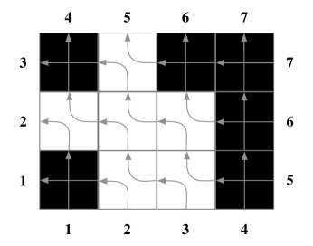
The connection between Cauchon diagrams and restricted permutations suggested by Theorems 2.4 and 3.1 can be made clear via a notion called pipe dreams. To explain this idea, let us fix an m×n𝑚𝑛m\times n diagram D𝐷D. We lay “pipes” on the squares of D𝐷D by placing a “hyperbola” on every white square and a “cross” on every black square (see Figure 2). Next, we label the sides of the diagram by elements of [m+n]delimited-[]𝑚𝑛[m+n] as in, for example, Figure 2 (we assume the general form of the labelling is obvious from this consideration).
Refer to caption
Figure 2. Example of applying pipe dreams to a given diagram

The restricted permutation σ𝜎\sigma is obtained from this process by defining σ(i)𝜎𝑖\sigma(i) to be the label (on the left or top side of D𝐷D) reached by following the pipe starting at label i𝑖i (on the bottom or right side of the D𝐷D). To be clear, when following a pipe through a black square, we always go straight through the square.

For example, in the diagram of Figure 2, we obtain the restricted permutation (1 2)( 3 4 7 5)123475(1\,2)(\,3\,4\,7\,5). Notice that the inverse of the permutation is obtained by reversing this procedure, that is, starting at a label from the left or top and following the pipe to the bottom or right of the diagram.

Definition 3.2.

We denote by ω𝜔\omega the restricted (m+n)𝑚𝑛(m+n)-permutation obtained from the m×n𝑚𝑛m\times n diagram consisting of only black squares. Therefore,

ω(i)={m+iif 1in,inif n+1in+m.𝜔𝑖cases𝑚𝑖if 1in,𝑖𝑛if n+1in+m.\omega(i)=\left\{\begin{array}[]{ll}m+i&\textnormal{if $1\leq i\leq n$,}\\ i-n&\textnormal{if $n+1\leq i\leq n+m$.}\end{array}\right.

The permutation ω𝜔\omega is the maximum element in the set of restricted (m+n)𝑚𝑛(m+n)-permutations ordered by the reverse Bruhat order.

4. Dimension of the \CH\C𝐻\C{H}-strata

In this section we prove Theorem 1.1.

4.1. Toric Permutations

We introduce the notion of toric permutations, which are essential in our analysis.

Definition 4.1.

Given a diagram D𝐷D with restricted permutation σ𝜎\sigma, the toric permutation associated to D𝐷D is simply the permutation τ=σω1𝜏𝜎superscript𝜔1\tau=\sigma\omega^{-1}.

The toric permutation can be obtained via pipe dreams simply by following the same procedure except the bottom and right sides of the diagram are now relabelled as in Figure 3. Notice that under this labelling, any cycle in the toric permutation may be found by considering the diagram as a “torus” and following the pipe around the “torus”.

Refer to caption
Figure 3. New row/column labelling to obtain the toric permutation (1 3 5)(2 6 4)(7)1352647(1\,3\,5)(2\,6\,4)(7)

The proof of Theorem 1.1 requires the following two lemmas. For a permutation μSk𝜇subscript𝑆𝑘\mu\in S_{k}, Pμsubscript𝑃𝜇P_{\mu} denotes the corresponding k×k𝑘𝑘k\times k permutation matrix. That is, Pμsubscript𝑃𝜇P_{\mu} is the k×k𝑘𝑘k\times k matrix whose entries are defined by Pμ[i,j]:=δj,σ(i)assignsubscript𝑃𝜇𝑖𝑗subscript𝛿𝑗𝜎𝑖P_{\mu}[i,j]:=\delta_{j,\sigma(i)}, where δ𝛿\delta denotes the Kronecker symbol.

Lemma 4.2.

Let D𝐷D be an m×n𝑚𝑛m\times n diagram whose corresponding restricted permutation is σ𝜎\sigma. If τ=σω1𝜏𝜎superscript𝜔1\tau=\sigma\omega^{-1} is the toric permutation associated to D𝐷D, then 𝐯ker(Pω+Pσ)𝐯kernelsubscript𝑃𝜔subscript𝑃𝜎{\boldsymbol{v}}\in\ker(P_{\omega}+P_{\sigma}) if and only if 𝐯b=𝐯τ(b)subscript𝐯𝑏subscript𝐯𝜏𝑏{\boldsymbol{v}}_{b}=-{\boldsymbol{v}}_{\tau(b)} for every label b𝑏b, where 𝐯isubscript𝐯𝑖{\boldsymbol{v}}_{i} denotes the i𝑖ith coordinate of 𝐯𝐯{\boldsymbol{v}}.

Proof.

Consider the pipe in D𝐷D corresponding to the cycle in τ𝜏\tau containing b𝑏b and τ(b)𝜏𝑏\tau(b). Now 𝒗ker(Pω+Pσ)𝒗kernelsubscript𝑃𝜔subscript𝑃𝜎{\boldsymbol{v}}\in\ker(P_{\omega}+P_{\sigma}) if and only if for all a𝑎a we have 𝒗ω(a)+𝒗σ(a)=0subscript𝒗𝜔𝑎subscript𝒗𝜎𝑎0{\boldsymbol{v}}_{\omega(a)}+{\boldsymbol{v}}_{\sigma(a)}=0. Taking a=ω1(b)𝑎superscript𝜔1𝑏a=\omega^{-1}(b) we obtain 𝒗b=𝒗τ(b)subscript𝒗𝑏subscript𝒗𝜏𝑏{\boldsymbol{v}}_{b}=-{\boldsymbol{v}}_{\tau(b)} as desired. ∎

Lemma 4.3.

Let D𝐷D be an m×n𝑚𝑛m\times n diagram whose corresponding restricted permutation is σ𝜎\sigma, and let τ𝜏\tau denote the toric permutation τ=σω1𝜏𝜎superscript𝜔1\tau=\sigma\omega^{-1}. Then the dimension of ker(Pω+Pσ)kernelsubscript𝑃𝜔subscript𝑃𝜎\ker(P_{\omega}+P_{\sigma}) is the number of odd cycles in the disjoint-cycle decomposition of τ𝜏\tau.

Proof.

Let {γ1,,γ}subscript𝛾1subscript𝛾\{\gamma_{1},\ldots,\gamma_{\ell}\} be the set of odd cycles in the disjoint cycle decomposition of σω1𝜎superscript𝜔1\sigma\omega^{-1}. Given the odd cycle γ=(a1a2a2k)𝛾subscript𝑎1subscript𝑎2subscript𝑎2𝑘\gamma=(a_{1}\,a_{2}\,\ldots\,a_{2k}), define the vector 𝒗γm+nsuperscript𝒗𝛾superscript𝑚𝑛{\boldsymbol{v}}^{\gamma}\in\mathbb{Z}^{m+n} by

𝒗bγ={1if b=ai and i is odd,1if b=ai and i is even,0otherwise.subscriptsuperscript𝒗𝛾𝑏cases1if b=ai and i is odd,1if b=ai and i is even,0otherwise.{\boldsymbol{v}}^{\gamma}_{b}=\left\{\begin{array}[]{ll}1&\textnormal{if $b=a_{i}$ and $i$ is odd,}\\ -1&\textnormal{if $b=a_{i}$ and $i$ is even,}\\ 0&\textnormal{otherwise.}\end{array}\right.

We claim that the set B={𝒗γii[]}𝐵conditional-setsuperscript𝒗subscript𝛾𝑖𝑖delimited-[]B=\{{\boldsymbol{v}}^{\gamma_{i}}\mid i\in[\ell]\} forms a basis for ker(Pω+Pσ)kernelsubscript𝑃𝜔subscript𝑃𝜎\ker(P_{\omega}+P_{\sigma}). Since the odd cycles are mutually disjoint, it is clear that the members of B𝐵B form an independent set in the \mathbb{Z}-module m+nsuperscript𝑚𝑛\mathbb{Z}^{m+n}.

Suppose that 𝒗ker(Pω+Pσ)𝒗kernelsubscript𝑃𝜔subscript𝑃𝜎{\boldsymbol{v}}\in\ker(P_{\omega}+P_{\sigma}). By Lemma 4.2, we know that if b𝑏b is in an even cycle of τ𝜏\tau, then 𝒗b=0subscript𝒗𝑏0{\boldsymbol{v}}_{b}=0. Moreover, the values of the entries corresponding to an odd cycle agree up to multiplication by 11-1. Thus we see that 𝒗𝒗{\boldsymbol{v}} can be written as a linear combination of elements of B𝐵B. ∎

4.2. Proof of Theorem 1.1

Notation 4.4.

Fix an m×n𝑚𝑛m\times n diagram D𝐷D with N𝑁N white squares labelled by distinct elements of the set [N]delimited-[]𝑁[N] such that labels are strictly increasing from left to right along rows and if i<j𝑖𝑗i<j then the label of each white box in row i𝑖i is strictly less than the label of each white box in row j𝑗j. Let τ=σω1𝜏𝜎superscript𝜔1\tau=\sigma\omega^{-1} be the toric permutation of D𝐷D. Let 𝒘𝒘{\boldsymbol{w}} be in the column space of M(D)𝑀𝐷M(D) and 𝒗𝒗{\boldsymbol{v}} in the column space of Pω+Pσsubscript𝑃𝜔subscript𝑃𝜎P_{\omega}+P_{\sigma}. We refer to the entries of 𝒘𝒘{\boldsymbol{w}} by 𝒘jsubscript𝒘𝑗{\boldsymbol{w}}_{j} for j[N]𝑗delimited-[]𝑁j\in[N] and the entries of 𝒗𝒗{\boldsymbol{v}} by 𝒗asubscript𝒗𝑎{\boldsymbol{v}}_{a} where a[m+n]𝑎delimited-[]𝑚𝑛a\in[m+n].

  1. (1)

    Since, in the toric labelling, each side of a row or column is given the same label, we may unambiguously refer to a row or column by this label.

  2. (2)

    Given a diagram D𝐷D with the toric labelling and a white square i𝑖i of D𝐷D, let left(i)left𝑖\textnormal{left}(i) and up(i)up𝑖\textnormal{up}(i) be, respectively, the labels of the rows or columns reached by following the bottom and top pipes of the hyperbola pipe placed on i𝑖i. See Example 4.5.

  3. (3)

    For S[N]𝑆delimited-[]𝑁S\subseteq[N], let 𝒘S=jS𝒘jsubscript𝒘𝑆subscript𝑗𝑆subscript𝒘𝑗{\boldsymbol{w}}_{S}=\sum_{j\in S}{\boldsymbol{w}}_{j}.

  4. (4)

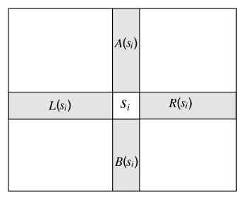
    For a given white square i𝑖i, let A(i),R(i),B(i)𝐴𝑖𝑅𝑖𝐵𝑖A(i),R(i),B(i) and L(i)𝐿𝑖L(i) be the sets of white squares that are, respectively, strictly above, strictly to the right, strictly below and strictly to the left of square i𝑖i.

Refer to caption
Figure 4.
Example 4.5.

Consider the diagram in Figure 4. For this example, we have labelled the white squares in a regular font, and the row and column labels in bold font. We have, for example, left(7)=𝟒left74\textnormal{left}(7)={\boldsymbol{4}} and up(7)=𝟕up77\textnormal{up}(7)={\boldsymbol{7}}, while left(8)=𝟕left87\textnormal{left}(8)={\boldsymbol{7}} and up(8)=𝟔up86\textnormal{up}(8)={\boldsymbol{6}}. On the other hand A(5)={2},R(5)=,B(5)={6,9}formulae-sequence𝐴52formulae-sequence𝑅5𝐵569A(5)=\{2\},R(5)=\emptyset,B(5)=\{6,9\} and L(5)={4}𝐿54L(5)=\{4\}.

Before proving the main theorem of this section, we note that by the definition of M(D)𝑀𝐷M(D) we have 𝒘ker(M(D))𝒘kernel𝑀𝐷{\boldsymbol{w}}\in\ker(M(D)) if and only if for every white square i𝑖i, the following identity holds

𝒘A(i)+𝒘L(i)=𝒘B(i)+𝒘R(i).subscript𝒘𝐴𝑖subscript𝒘𝐿𝑖subscript𝒘𝐵𝑖subscript𝒘𝑅𝑖{\boldsymbol{w}}_{A(i)}+{\boldsymbol{w}}_{L(i)}={\boldsymbol{w}}_{B(i)}+{\boldsymbol{w}}_{R(i)}.
Theorem 4.6.

If D𝐷D is a diagram and σ𝜎\sigma is the restricted permutation obtained from D𝐷D, then

ker(Pω+Pσ)ker(M(D)).similar-to-or-equalskernelsubscript𝑃𝜔subscript𝑃𝜎kernel𝑀𝐷\ker(P_{\omega}+P_{\sigma})\simeq\ker(M(D)).
Proof.

We place the toric labelling on D𝐷D. Suppose that D𝐷D has N𝑁N white squares labelled 1,2,,N12𝑁1,2,\ldots,N. The theorem is proved once we exhibit injective functions ϕ:ker(Pω+Pσ)ker(M(D)):italic-ϕkernelsubscript𝑃𝜔subscript𝑃𝜎kernel𝑀𝐷\phi:\ker(P_{\omega}+P_{\sigma})\rightarrow\ker(M(D)) and ψ:ker(M(D))ker(Pω+Pσ):𝜓kernel𝑀𝐷kernelsubscript𝑃𝜔subscript𝑃𝜎\psi:\ker(M(D))\rightarrow\ker(P_{\omega}+P_{\sigma}). The reader may wish to refer to the example immediately following this proof where we give an explicit calculation of ϕitalic-ϕ\phi and ψ𝜓\psi for the diagram of Figure 4.

Given 𝒗ker(Pω+Pσ)𝒗kernelsubscript𝑃𝜔subscript𝑃𝜎{\boldsymbol{v}}\in\ker(P_{\omega}+P_{\sigma}), we take 𝒘:=ϕ(𝒗){\boldsymbol{w}}:=\phi({\boldsymbol{v}}) to be the vector whose entries are defined by 𝒘i=𝒗left(i)𝒗up(i)subscript𝒘𝑖subscript𝒗left𝑖subscript𝒗up𝑖{\boldsymbol{w}}_{i}={\boldsymbol{v}}_{\textnormal{left}(i)}-{\boldsymbol{v}}_{\textnormal{up}(i)}. To show 𝒘ker(M(D))𝒘kernel𝑀𝐷{\boldsymbol{w}}\in\ker(M(D)) we need only to check that for all white squares i𝑖i the relation 𝒘A(i)+𝒘L(i)𝒘B(i)𝒘R(i)=0subscript𝒘𝐴𝑖subscript𝒘𝐿𝑖subscript𝒘𝐵𝑖subscript𝒘𝑅𝑖0{\boldsymbol{w}}_{A(i)}+{\boldsymbol{w}}_{L(i)}-{\boldsymbol{w}}_{B(i)}-{\boldsymbol{w}}_{R(i)}=0 holds.

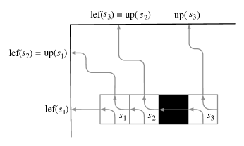
Notice that, if S={s1,s2,,sk}𝑆subscript𝑠1subscript𝑠2subscript𝑠𝑘S=\{s_{1},s_{2},\ldots,s_{k}\} is any block of consecutive white squares in the same row, where s1subscript𝑠1s_{1} is the left-most white square, and sksubscript𝑠𝑘s_{k} is the right-most, then we have 𝒘S=𝒗left(s1)𝒗up(sk)subscript𝒘𝑆subscript𝒗leftsubscript𝑠1subscript𝒗upsubscript𝑠𝑘{\boldsymbol{w}}_{S}={\boldsymbol{v}}_{\textnormal{left}(s_{1})}-{\boldsymbol{v}}_{\textnormal{up}(s_{k})} since one can easily check that up(si)=left(si+1)upsubscript𝑠𝑖leftsubscript𝑠𝑖1\textnormal{up}(s_{i})=\textnormal{left}(s_{i+1}) for i[k1]𝑖delimited-[]𝑘1i\in[k-1]. For a small example, see Figure 5.

Refer to caption
Figure 5. 𝒘{s1,s2,s3}=𝒗left(s1)𝒗up(s3)subscript𝒘subscript𝑠1subscript𝑠2subscript𝑠3subscript𝒗leftsubscript𝑠1subscript𝒗upsubscript𝑠3{\boldsymbol{w}}_{\{s_{1},s_{2},s_{3}\}}={\boldsymbol{v}}_{\textnormal{left}(s_{1})}-{\boldsymbol{v}}_{\textnormal{up}(s_{3})}

Similarly, if S={s1,s2,,sk}𝑆subscript𝑠1subscript𝑠2subscript𝑠𝑘S=\{s_{1},s_{2},\ldots,s_{k}\} is any block of consecutive white squares in the same column, where s1subscript𝑠1s_{1} is the bottom-most white square, and sksubscript𝑠𝑘s_{k} is the top-most white square, then 𝒘S=𝒗left(s1)𝒗up(sk)subscript𝒘𝑆subscript𝒗leftsubscript𝑠1subscript𝒗upsubscript𝑠𝑘{\boldsymbol{w}}_{S}={\boldsymbol{v}}_{\textnormal{left}(s_{1})}-{\boldsymbol{v}}_{\textnormal{up}(s_{k})}.

Fix a white square i𝑖i. For the sake of brevity, we assume that A(i),L(i),B(i)𝐴𝑖𝐿𝑖𝐵𝑖A(i),L(i),B(i) and R(i)𝑅𝑖R(i) are all non-empty; the remaining cases are similar. We now show that 𝒘A(i)+𝒘L(i)𝒘B(i)𝒘R(i)=0subscript𝒘𝐴𝑖subscript𝒘𝐿𝑖subscript𝒘𝐵𝑖subscript𝒘𝑅𝑖0{\boldsymbol{w}}_{A(i)}+{\boldsymbol{w}}_{L(i)}-{\boldsymbol{w}}_{B(i)}-{\boldsymbol{w}}_{R(i)}=0 (Figure 6). Suppose that the label of the row containing i𝑖i is r𝑟r and the label of the column containing i𝑖i is c𝑐c. Let sr,1subscript𝑠𝑟1s_{r,1} be the left-most white square in row r𝑟r, sr,ksubscript𝑠𝑟𝑘s_{r,k} the right-most white square in row r𝑟r, sc,1subscript𝑠𝑐1s_{c,1} the bottom-most white square in column c𝑐c and sc,subscript𝑠𝑐s_{c,\ell} the top-most white square in column c𝑐c.

Refer to caption
Figure 6.

We have

𝒘A(i)+𝒘L(i)𝒘B(i)𝒘R(i)subscript𝒘𝐴𝑖subscript𝒘𝐿𝑖subscript𝒘𝐵𝑖subscript𝒘𝑅𝑖\displaystyle{\boldsymbol{w}}_{A(i)}+{\boldsymbol{w}}_{L(i)}-{\boldsymbol{w}}_{B(i)}-{\boldsymbol{w}}_{R(i)} =\displaystyle= (𝒗up(i)𝒗up(sc,))+(𝒗left(sr,1)𝒗left(i))subscript𝒗up𝑖subscript𝒗upsubscript𝑠𝑐subscript𝒗leftsubscript𝑠𝑟1subscript𝒗left𝑖\displaystyle({\boldsymbol{v}}_{\textnormal{up}(i)}-{\boldsymbol{v}}_{\textnormal{up}(s_{c,\ell})})+({\boldsymbol{v}}_{\textnormal{left}(s_{r,1})}-{\boldsymbol{v}}_{\textnormal{left}(i)})
(𝒗left(sc,1)𝒗left(i))(𝒗up(i)𝒗up(sr,k))subscript𝒗leftsubscript𝑠𝑐1subscript𝒗left𝑖subscript𝒗up𝑖subscript𝒗upsubscript𝑠𝑟𝑘\displaystyle-({\boldsymbol{v}}_{\textnormal{left}(s_{c,1})}-{\boldsymbol{v}}_{\textnormal{left}(i)})-({\boldsymbol{v}}_{\textnormal{up}(i)}-{\boldsymbol{v}}_{\textnormal{up}(s_{r,k})})
=\displaystyle= (𝒗left(sr,1)+𝒗up(sr,k))(𝒗up(sc,1)+𝒗left(sc,))subscript𝒗leftsubscript𝑠𝑟1subscript𝒗upsubscript𝑠𝑟𝑘subscript𝒗upsubscript𝑠𝑐1subscript𝒗leftsubscript𝑠𝑐\displaystyle({\boldsymbol{v}}_{\textnormal{left}(s_{r,1})}+{\boldsymbol{v}}_{\textnormal{up}(s_{r,k})})-({\boldsymbol{v}}_{\textnormal{up}(s_{c,1})}+{\boldsymbol{v}}_{\textnormal{left}(s_{c,\ell})})
=\displaystyle= (𝒗r+𝒗τ(r))(𝒗c+𝒗τ(c))subscript𝒗𝑟subscript𝒗𝜏𝑟subscript𝒗𝑐subscript𝒗𝜏𝑐\displaystyle({\boldsymbol{v}}_{r}+{\boldsymbol{v}}_{\tau(r)})-({\boldsymbol{v}}_{c}+{\boldsymbol{v}}_{\tau(c)})
=\displaystyle= 0,0\displaystyle 0,

where the last equality follows by Lemma 4.2.

Now define ψ:ker(M(D))ker(Pω+Pσ):𝜓kernel𝑀𝐷kernelsubscript𝑃𝜔subscript𝑃𝜎\psi:\ker(M(D))\rightarrow\ker(P_{\omega}+P_{\sigma}) as follows. Let 𝒘ker(M(D))𝒘kernel𝑀𝐷{\boldsymbol{w}}\in\ker(M(D)) and write 𝒗=ψ(𝒘)𝒗𝜓𝒘{\boldsymbol{v}}=\psi({\boldsymbol{w}}). If a𝑎a is a column we take 𝒗asubscript𝒗𝑎{\boldsymbol{v}}_{a} to be the sum of all white squares in column a𝑎a, but if a𝑎a is a row, then we take 𝒗asubscript𝒗𝑎{\boldsymbol{v}}_{a} to be the negative of the sum of all white squares in row a𝑎a. By Lemma 4.2, we want to show that for all labels a𝑎a, we have

(1) 𝒗a+𝒗τ(a)subscript𝒗𝑎subscript𝒗𝜏𝑎\displaystyle{\boldsymbol{v}}_{a}+{\boldsymbol{v}}_{\tau(a)} =\displaystyle= 0.0\displaystyle 0.

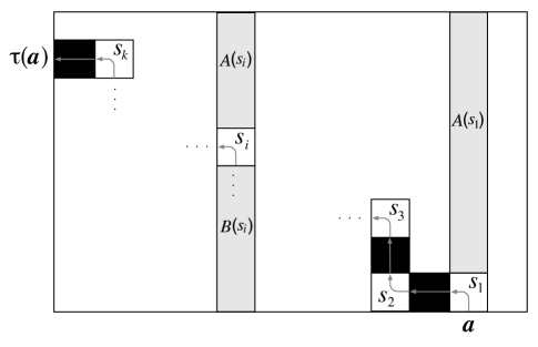
Fix a label a[m+n]𝑎delimited-[]𝑚𝑛a\in[m+n] and let (s1,s2,,sk)subscript𝑠1subscript𝑠2subscript𝑠𝑘(s_{1},s_{2},\ldots,s_{k}) be the sequence of white squares used in the pipe from a𝑎a to τ(a)𝜏𝑎\tau(a).

Refer to caption
Figure 7.

We assume that a𝑎a is a column as the case in which a𝑎a is a row is argued similarly. We first prove by induction that, for every i=1,,k𝑖1𝑘i=1,\ldots,k, we have

(2) 𝒗asubscript𝒗𝑎\displaystyle{\boldsymbol{v}}_{a} =\displaystyle= 𝒘s1+𝒘A(s1)subscript𝒘subscript𝑠1subscript𝒘𝐴subscript𝑠1\displaystyle{\boldsymbol{w}}_{s_{1}}+{\boldsymbol{w}}_{A(s_{1})}
=\displaystyle= (1)i+1𝒘si+𝒘A(si)𝒘B(si).superscript1𝑖1subscript𝒘subscript𝑠𝑖subscript𝒘𝐴subscript𝑠𝑖subscript𝒘𝐵subscript𝑠𝑖\displaystyle(-1)^{i+1}{\boldsymbol{w}}_{s_{i}}+{\boldsymbol{w}}_{A(s_{i})}-{\boldsymbol{w}}_{B(s_{i})}.

See Figure 7. If i=1𝑖1i=1, then Equation (2) is trivially true since B(si)=𝐵subscript𝑠𝑖B(s_{i})=\emptyset. So suppose that it is true for all values less than i>1𝑖1i>1. There are two cases to consider. If i𝑖i is even, then sisubscript𝑠𝑖s_{i} is the first white square to the left of si1subscript𝑠𝑖1s_{i-1}. Note that 𝒘R(si)=𝒘R(si1)+𝒘si1subscript𝒘𝑅subscript𝑠𝑖subscript𝒘𝑅subscript𝑠𝑖1subscript𝒘subscript𝑠𝑖1{\boldsymbol{w}}_{R(s_{i})}={\boldsymbol{w}}_{R(s_{i-1})}+{\boldsymbol{w}}_{s_{i-1}} and 𝒘L(si1)=𝒘L(si)+𝒘sisubscript𝒘𝐿subscript𝑠𝑖1subscript𝒘𝐿subscript𝑠𝑖subscript𝒘subscript𝑠𝑖{\boldsymbol{w}}_{L(s_{i-1})}={\boldsymbol{w}}_{L(s_{i})}+{\boldsymbol{w}}_{s_{i}}. Since 𝒘ker(M(D))𝒘kernel𝑀𝐷{\boldsymbol{w}}\in\ker(M(D)) we have the two equations

𝒘A(si1)+𝒘L(si)+𝒘si𝒘B(si1)𝒘R(si1)=0,subscript𝒘𝐴subscript𝑠𝑖1subscript𝒘𝐿subscript𝑠𝑖subscript𝒘subscript𝑠𝑖subscript𝒘𝐵subscript𝑠𝑖1subscript𝒘𝑅subscript𝑠𝑖10{\boldsymbol{w}}_{A(s_{i-1})}+{\boldsymbol{w}}_{L(s_{i})}+{\boldsymbol{w}}_{s_{i}}-{\boldsymbol{w}}_{B(s_{i-1})}-{\boldsymbol{w}}_{R(s_{i-1})}=0,

and

𝒘A(si)+𝒘L(si)𝒘B(si)𝒘R(si1)𝒘si1=0.subscript𝒘𝐴subscript𝑠𝑖subscript𝒘𝐿subscript𝑠𝑖subscript𝒘𝐵subscript𝑠𝑖subscript𝒘𝑅subscript𝑠𝑖1subscript𝒘subscript𝑠𝑖10{\boldsymbol{w}}_{A(s_{i})}+{\boldsymbol{w}}_{L(s_{i})}-{\boldsymbol{w}}_{B(s_{i})}-{\boldsymbol{w}}_{R(s_{i-1})}-{\boldsymbol{w}}_{s_{i-1}}=0.

Subtracting the second equation from the first we obtain

(3) 𝒘si1+𝒘A(si1)𝒘B(si1)subscript𝒘subscript𝑠𝑖1subscript𝒘𝐴subscript𝑠𝑖1subscript𝒘𝐵subscript𝑠𝑖1\displaystyle{\boldsymbol{w}}_{s_{i-1}}+{\boldsymbol{w}}_{A(s_{i-1})}-{\boldsymbol{w}}_{B(s_{i-1})} =\displaystyle= 𝒘si+𝒘A(si)𝒘B(si).subscript𝒘subscript𝑠𝑖subscript𝒘𝐴subscript𝑠𝑖subscript𝒘𝐵subscript𝑠𝑖\displaystyle-{\boldsymbol{w}}_{s_{i}}+{\boldsymbol{w}}_{A(s_{i})}-{\boldsymbol{w}}_{B(s_{i})}.

But since i1𝑖1i-1 is odd, the left hand side of (3) is equal, by induction, to 𝒘s1+𝒘A(s1)subscript𝒘subscript𝑠1subscript𝒘𝐴subscript𝑠1{\boldsymbol{w}}_{s_{1}}+{\boldsymbol{w}}_{A(s_{1})} and thus (3) implies (2) for the case that i𝑖i is even.

Now for i𝑖i odd, sisubscript𝑠𝑖s_{i} is the first white square above si1subscript𝑠𝑖1s_{i-1}. It is easy to check that we have the two equations

𝒘A(si1)=𝒘A(si)+𝒘sisubscript𝒘𝐴subscript𝑠𝑖1subscript𝒘𝐴subscript𝑠𝑖subscript𝒘subscript𝑠𝑖{\boldsymbol{w}}_{A(s_{i-1})}={\boldsymbol{w}}_{A(s_{i})}+{\boldsymbol{w}}_{s_{i}}

and

𝒘B(si)=𝒘B(si1)+𝒘si1.subscript𝒘𝐵subscript𝑠𝑖subscript𝒘𝐵subscript𝑠𝑖1subscript𝒘subscript𝑠𝑖1{\boldsymbol{w}}_{B(s_{i})}={\boldsymbol{w}}_{B(s_{i-1})}+{\boldsymbol{w}}_{s_{i-1}}.

By induction we obtain

𝒘s1+𝒘A(s1)subscript𝒘subscript𝑠1subscript𝒘𝐴subscript𝑠1\displaystyle{\boldsymbol{w}}_{s_{1}}+{\boldsymbol{w}}_{A(s_{1})} =\displaystyle= 𝒘si1+𝒘A(si1)𝒘B(si1)subscript𝒘subscript𝑠𝑖1subscript𝒘𝐴subscript𝑠𝑖1subscript𝒘𝐵subscript𝑠𝑖1\displaystyle-{\boldsymbol{w}}_{s_{i-1}}+{\boldsymbol{w}}_{A(s_{i-1})}-{\boldsymbol{w}}_{B(s_{i-1})}
=\displaystyle= 𝒘si1+𝒘A(si)+𝒘si(𝒘B(si)𝒘si1)subscript𝒘subscript𝑠𝑖1subscript𝒘𝐴subscript𝑠𝑖subscript𝒘subscript𝑠𝑖subscript𝒘𝐵subscript𝑠𝑖subscript𝒘subscript𝑠𝑖1\displaystyle-{\boldsymbol{w}}_{s_{i-1}}+{\boldsymbol{w}}_{A(s_{i})}+{\boldsymbol{w}}_{s_{i}}-({\boldsymbol{w}}_{B(s_{i})}-{\boldsymbol{w}}_{s_{i-1}})
=\displaystyle= 𝒘si+𝒘A(si)𝒘B(si).subscript𝒘subscript𝑠𝑖subscript𝒘𝐴subscript𝑠𝑖subscript𝒘𝐵subscript𝑠𝑖\displaystyle{\boldsymbol{w}}_{s_{i}}+{\boldsymbol{w}}_{A(s_{i})}-{\boldsymbol{w}}_{B(s_{i})}.

This finishes the proof of Equation (2).

Now we verify Equation (1). If k𝑘k is even, then τ(a)𝜏𝑎\tau(a) is a column-label and so A(sk)=𝐴subscript𝑠𝑘A(s_{k})=\emptyset. By (2),

𝒗asubscript𝒗𝑎\displaystyle{\boldsymbol{v}}_{a} =\displaystyle= 𝒘s1+𝒘A(s1)subscript𝒘subscript𝑠1subscript𝒘𝐴subscript𝑠1\displaystyle{\boldsymbol{w}}_{s_{1}}+{\boldsymbol{w}}_{A(s_{1})}
=\displaystyle= 𝒘sk+𝒘A(sk)𝒘B(sk)subscript𝒘subscript𝑠𝑘subscript𝒘𝐴subscript𝑠𝑘subscript𝒘𝐵subscript𝑠𝑘\displaystyle-{\boldsymbol{w}}_{s_{k}}+{\boldsymbol{w}}_{A(s_{k})}-{\boldsymbol{w}}_{B(s_{k})}
=\displaystyle= 𝒘sk𝒘B(sk)subscript𝒘subscript𝑠𝑘subscript𝒘𝐵subscript𝑠𝑘\displaystyle-{\boldsymbol{w}}_{s_{k}}-{\boldsymbol{w}}_{B(s_{k})}
=\displaystyle= 𝒗τ(a).subscript𝒗𝜏𝑎\displaystyle-{\boldsymbol{v}}_{\tau(a)}.

On the other hand, if k𝑘k is odd, then τ(a)𝜏𝑎\tau(a) is a row-label and so L(sk)=𝐿subscript𝑠𝑘L(s_{k})=\emptyset. Since 𝒘ker(M(D))𝒘kernel𝑀𝐷{\boldsymbol{w}}\in\ker(M(D)), we must have 𝒘A(sk)𝒘B(sk)=𝒘R(sk)subscript𝒘𝐴subscript𝑠𝑘subscript𝒘𝐵subscript𝑠𝑘subscript𝒘𝑅subscript𝑠𝑘{\boldsymbol{w}}_{A(s_{k})}-{\boldsymbol{w}}_{B(s_{k})}={\boldsymbol{w}}_{R(s_{k})}. Hence

𝒗asubscript𝒗𝑎\displaystyle{\boldsymbol{v}}_{a} =\displaystyle= 𝒘s1+𝒘A(s1)subscript𝒘subscript𝑠1subscript𝒘𝐴subscript𝑠1\displaystyle{\boldsymbol{w}}_{s_{1}}+{\boldsymbol{w}}_{A(s_{1})}
=\displaystyle= 𝒘sk+𝒘A(sk)𝒘B(sk)subscript𝒘subscript𝑠𝑘subscript𝒘𝐴subscript𝑠𝑘subscript𝒘𝐵subscript𝑠𝑘\displaystyle{\boldsymbol{w}}_{s_{k}}+{\boldsymbol{w}}_{A(s_{k})}-{\boldsymbol{w}}_{B(s_{k})}
=\displaystyle= 𝒘sk+𝒘R(sk)subscript𝒘subscript𝑠𝑘subscript𝒘𝑅subscript𝑠𝑘\displaystyle{\boldsymbol{w}}_{s_{k}}+{\boldsymbol{w}}_{R(s_{k})}
=\displaystyle= 𝒗τ(a).subscript𝒗𝜏𝑎\displaystyle-{\boldsymbol{v}}_{\tau(a)}.

The final step is to prove that the functions ϕitalic-ϕ\phi and ψ𝜓\psi are injective. First, suppose that ψ(𝒘)=𝟎𝜓𝒘0\psi({\boldsymbol{w}})={\boldsymbol{0}} with 𝒘𝟎𝒘0{\boldsymbol{w}}\neq{\boldsymbol{0}}. There must, therefore, exist a white square i𝑖i (with i𝑖i minimum) such that 𝒘i0subscript𝒘𝑖0{\boldsymbol{w}}_{i}\neq 0 but 𝒘A(i)=0subscript𝒘𝐴𝑖0{\boldsymbol{w}}_{A(i)}=0 and 𝒘L(i)=0subscript𝒘𝐿𝑖0{\boldsymbol{w}}_{L(i)}=0. Since 𝒘ker(M(D))𝒘kernel𝑀𝐷{\boldsymbol{w}}\in\ker(M(D)) we have 𝒘B(i)+𝒘R(i)=0subscript𝒘𝐵𝑖subscript𝒘𝑅𝑖0{\boldsymbol{w}}_{B(i)}+{\boldsymbol{w}}_{R(i)}=0. On the other hand, since ψ(𝒘)=𝟎𝜓𝒘0\psi({\boldsymbol{w}})={\boldsymbol{0}} we have, by the construction of ψ(𝒘)𝜓𝒘\psi({\boldsymbol{w}}), that 𝒘B(i)+𝒘i=0subscript𝒘𝐵𝑖subscript𝒘𝑖0{\boldsymbol{w}}_{B(i)}+{\boldsymbol{w}}_{i}=0 and 0=𝒘R(i)+𝒘i=𝒘B(i)+𝒘i0subscript𝒘𝑅𝑖subscript𝒘𝑖subscript𝒘𝐵𝑖subscript𝒘𝑖0={\boldsymbol{w}}_{R(i)}+{\boldsymbol{w}}_{i}=-{\boldsymbol{w}}_{B(i)}+{\boldsymbol{w}}_{i}. Thus we must have 𝒘i=0subscript𝒘𝑖0{\boldsymbol{w}}_{i}=0, contradicting the choice of i𝑖i. Therefore ψ𝜓\psi is injective.

To show that ϕitalic-ϕ\phi is injective we show that ψ(ϕ(𝒗))=2𝒗𝜓italic-ϕ𝒗2𝒗\psi(\phi({\boldsymbol{v}}))=-2{\boldsymbol{v}} for every 𝒗ker(Pω+Pσ)𝒗kernelsubscript𝑃𝜔subscript𝑃𝜎{\boldsymbol{v}}\in\ker(P_{\omega}+P_{\sigma}). First, if a𝑎a is a row then

ψ(ϕ(𝒗))a=i in column aϕ(𝒗)i=i in column a(𝒗left(i)𝒗up(i))=(𝒗a𝒗τ(a)).𝜓subscriptitalic-ϕ𝒗𝑎subscript𝑖 in column 𝑎italic-ϕsubscript𝒗𝑖subscript𝑖 in column 𝑎subscript𝒗left𝑖subscript𝒗up𝑖subscript𝒗𝑎subscript𝒗𝜏𝑎\psi(\phi({\boldsymbol{v}}))_{a}=-\sum_{i\mbox{ in column }a}\phi({\boldsymbol{v}})_{i}=-\sum_{i\mbox{ in column }a}({\boldsymbol{v}}_{\textnormal{left}(i)}-{\boldsymbol{v}}_{\textnormal{up}(i)})=-({\boldsymbol{v}}_{a}-{\boldsymbol{v}}_{\tau(a)}).

On the other hand, by Lemma 4.2, we know that 𝒗τ(a)=𝒗asubscript𝒗𝜏𝑎subscript𝒗𝑎{\boldsymbol{v}}_{\tau(a)}=-{\boldsymbol{v}}_{a} and thus ψ(ϕ(𝒗))a=2𝒗a𝜓subscriptitalic-ϕ𝒗𝑎2subscript𝒗𝑎\psi(\phi({\boldsymbol{v}}))_{a}=-2{\boldsymbol{v}}_{a}. A similar argument shows that if a𝑎a is a column then ψ(ϕ(𝒗))a=2𝒗a𝜓subscriptitalic-ϕ𝒗𝑎2subscript𝒗𝑎\psi(\phi({\boldsymbol{v}}))_{a}=-2{\boldsymbol{v}}_{a}. Hence ϕitalic-ϕ\phi is injective. ∎

Remark 1.

The linear maps ϕitalic-ϕ\phi and ψ𝜓\psi defined in the proof of Theorem 4.6 are not inverses. However one can check that

ψϕ=2id|ker(Pω+Pσ) and ϕψ=2id|ker(M(D)).𝜓italic-ϕevaluated-at2idkersubscript𝑃𝜔subscript𝑃𝜎 and italic-ϕ𝜓evaluated-at2idker𝑀𝐷\psi\circ\phi=-2\cdot{\rm id}|_{{\rm ker}(P_{\omega}+P_{\sigma})}\mbox{ and }\phi\circ\psi=-2\cdot{\rm id}|_{{\rm ker}(M(D))}.
Example 4.7.

In this example we give examples of the maps ϕitalic-ϕ\phi and ψ𝜓\psi from the above proof. If M𝑀M is a matrix, then Mtsuperscript𝑀𝑡M^{t} denotes its transpose. We consider the diagram from Figure 4. The corresponding toric permutation is (1 4 8 7 2 6)(3 5)14872635(1\,4\,8\,7\,2\,6)(3\,5). By Lemma 4.3, we may construct 𝒗=(1,1,0,1,0,1,1,1)t𝒗superscript11010111𝑡{\boldsymbol{v}}=(1,1,0,-1,0,-1,-1,1)^{t} corresponding to the cycle (1 4 8 7 2 6)148726(1\,4\,8\,7\,2\,6), and 𝒗:=(0,0,1,0,1,0,0,0)t{\boldsymbol{v}^{\prime}}:=(0,0,1,0,-1,0,0,0)^{t} corresponding to the cycle (3 5)35(3\,5).

Refer to caption
Figure 8. Calculating ϕ((1,1,0,1,0,1,1,1)t)italic-ϕsuperscript11010111𝑡\phi((1,1,0,-1,0,-1,-1,1)^{t})

In Figure 8, we now replaced the row or column-label i𝑖i with 𝒗isubscript𝒗𝑖{\boldsymbol{v}}_{i}. We wish to construct an element ϕ(𝒗)=𝒘italic-ϕ𝒗𝒘\phi({\boldsymbol{v}})={\boldsymbol{w}} in ker((M(D))\ker((M(D)). By the isomorphism in the proof of Theorem 4.6, we see that, for example, 𝒘8=𝒗left(8)𝒗up(8)=1(1)=0subscript𝒘8subscript𝒗left8subscript𝒗up8110{\boldsymbol{w}}_{8}={\boldsymbol{v}}_{\textnormal{left}(8)}-{\boldsymbol{v}}_{\textnormal{up}(8)}=-1-(-1)=0. Continuing in this way, we find that 𝒘=(1,1,2,1,1,2,0,0,0,2)t𝒘superscript1121120002𝑡{\boldsymbol{w}}=(-1,1,-2,1,-1,2,0,0,0,2)^{t}.

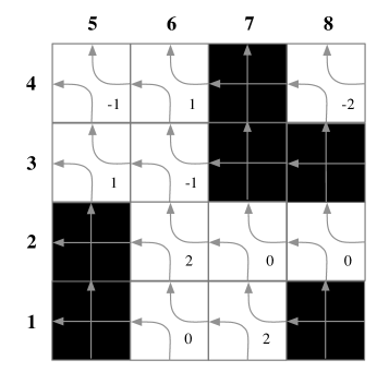
In Figure 9, we have replaced the white square labels from Figure 4 with the corresponding value of 𝒘𝒘{\boldsymbol{w}}. Using this, let us calculate ψ(𝒘)=𝒖𝜓𝒘𝒖\psi({\boldsymbol{w}})={\boldsymbol{u}}. This is easier: if i𝑖i is a row, then 𝒖isubscript𝒖𝑖{\boldsymbol{u}}_{i} is simply the negative of the row sum, and if i𝑖i is a column, then 𝒖isubscript𝒖𝑖{\boldsymbol{u}}_{i} is the column sum. Thus we obtain, 𝒖=(2,2,0,2,0,2,2,2)t𝒖superscript22020222𝑡{\boldsymbol{u}}=(-2,-2,0,2,0,2,2,-2)^{t}. It is easy to check that 𝒖=2𝒗ker(Pσ+Pω)𝒖2𝒗kernelsubscript𝑃𝜎subscript𝑃𝜔{\boldsymbol{u}}=-2{\boldsymbol{v}}\in\ker(P_{\sigma}+P_{\omega}).

Refer to caption
Figure 9. Calculating ψ((1,1,2,1,1,2,0,0,0,2)t).𝜓superscript1121120002𝑡\psi((-1,1,-2,1,-1,2,0,0,0,2)^{t}).
Corollary 4.8.

For a Cauchon diagram D𝐷D, the dimension of the \CH\C𝐻\C{H}-stratum corresponding to D𝐷D is equal to the number of odd cycles in the disjoint cycle decomposition of the toric permutation associated to D𝐷D.

Proof.

This follows immediately from Theorems 2.5 and 4.6. ∎

5. Enumeration of \CH\C𝐻\C{H}-primes with respect to dimension

In this section we apply Corollary 4.8 to obtain enumeration formulas for the total number of m×n𝑚𝑛m\times n \mathcal{H}-strata of a given dimension.

Suppose that we are given an m×n𝑚𝑛m\times n diagram D𝐷D with the property that the disjoint cycle decomposition of the toric permutation τ𝜏\tau consists of exactly one cycle τ=(a1a2am+n)𝜏subscript𝑎1subscript𝑎2subscript𝑎𝑚𝑛\tau=(a_{1}\,a_{2}\,\ldots\,a_{m+n}). Without loss of generality, take a1=1subscript𝑎11a_{1}=1. Using the pipe-dreams visualization of τ𝜏\tau, it is easy to check that the sequence (a1,a2,,am+n)subscript𝑎1subscript𝑎2subscript𝑎𝑚𝑛(a_{1},a_{2},\ldots,a_{m+n}) consists of contigious subsequences R1,C1,,Rk,Cksubscript𝑅1subscript𝐶1subscript𝑅𝑘subscript𝐶𝑘R_{1},C_{1},\ldots,R_{k},C_{k} alternating between increasing sets of row-labels (the Ri)R_{i}) and decreasing sets of column-labels (the Cisubscript𝐶𝑖C_{i}). In other words, we may write τ=(R1,C1,R2,,Rk,Ck)𝜏subscript𝑅1subscript𝐶1subscript𝑅2subscript𝑅𝑘subscript𝐶𝑘\tau=(R_{1},C_{1},R_{2},\ldots,R_{k},C_{k}) where the Risubscript𝑅𝑖R_{i} form a partition of [m]delimited-[]𝑚[m] and each Risubscript𝑅𝑖R_{i} is written in increasing order, while the Cisubscript𝐶𝑖C_{i} form a partition of m+[n]𝑚delimited-[]𝑛m+[n] and each Cisubscript𝐶𝑖C_{i} is written in decreasing order. We call τ𝜏\tau a toric cycle.

On the other hand, given a toric cycle τ=(R1,C1,R2,,Rk,Ck)𝜏subscript𝑅1subscript𝐶1subscript𝑅2subscript𝑅𝑘subscript𝐶𝑘\tau=(R_{1},C_{1},R_{2},\ldots,R_{k},C_{k}), it is a simple matter to check that the permutation τω𝜏𝜔\tau\omega is restricted in the sense of Section 3. By Theorems 2.4 and 3.1, we conclude that there exists a unique Cauchon diagram whose toric permutation is τ𝜏\tau.

Definition 5.1.

The number of partitions of [n]delimited-[]𝑛[n] into k𝑘k non-empty parts is the Stirling number of the second kind, and will here be denoted by {nk}FRACOP𝑛𝑘{n\brace k}. Note that some authors write S(n,k)𝑆𝑛𝑘S(n,k) for {nk}FRACOP𝑛𝑘{n\brace k}.

The above discussion implies that the number dm,nsubscript𝑑𝑚𝑛d_{m,n} of m×n𝑚𝑛m\times n diagrams whose toric permutation consists of exactly one cycle is exactly

dm,n=k=1min(m,n)k!(k1)!{mk}{nk}.subscript𝑑𝑚𝑛superscriptsubscript𝑘1𝑚𝑛𝑘𝑘1FRACOP𝑚𝑘FRACOP𝑛𝑘d_{m,n}=\sum_{k=1}^{\min(m,n)}k!(k-1)!{m\brace k}{n\brace k}.

Let 𝒟(x,y):=m,n1dm,nxmm!ynn!assign𝒟𝑥𝑦subscript𝑚𝑛1subscript𝑑𝑚𝑛superscript𝑥𝑚𝑚superscript𝑦𝑛𝑛\mathcal{D}(x,y):=\sum_{m,n\geq 1}d_{m,n}\frac{x^{m}}{m!}\frac{y^{n}}{n!} be the exponential generating function of dm,nsubscript𝑑𝑚𝑛d_{m,n} and let C(x,y)𝐶𝑥𝑦C(x,y) be the exponential generating function of all toric permutations (and hence of Cauchon diagrams). The relation between these two generating functions is provided to us via the well-known exponential formula. Note that while this formula is given in Section 5.1 of Stanley [16] (see also Chapter 3 in Wilf [17]) for single variable exponential generating functions, it is straightforward to generalize the result to multivariable exponential generating functions.

For those readers unfamiliar with the exponential formula, we now roughly describe the approach. Suppose we wish to find the exponential generating function A(x,y)𝐴𝑥𝑦A(x,y) of a set of a structures, where each structure can be written uniquely as a disjoint union of labelled “irreducible” components. For example, in the case that is of interest to us, the “structures” are the toric permutations, and the labelled irreducible components are the toric cycles. The exponential formula says that if B(x,y)𝐵𝑥𝑦B(x,y) is the exponential generating function for the labelled irreducible components, then A(x,y)=exp(B(x,y))𝐴𝑥𝑦𝐵𝑥𝑦A(x,y)=\exp(B(x,y)). In our case then, we obtain the following formula.

(4) C(x,y)𝐶𝑥𝑦\displaystyle C(x,y) =\displaystyle= exp(x+y)exp(𝒟(x,y)),𝑥𝑦𝒟𝑥𝑦\displaystyle\exp(x+y)\exp(\mathcal{D}(x,y)),

where the extra exp(x+y)𝑥𝑦\exp(x+y) is the exponential generating function for the all-black diagrams (i.e., the identity toric permutation).

We may refine 𝒟(x,y)𝒟𝑥𝑦\mathcal{D}(x,y) by noting that

𝒟e(x,y)=12(𝒟(x,y)𝒟(x,y))subscript𝒟𝑒𝑥𝑦12𝒟𝑥𝑦𝒟𝑥𝑦\mathcal{D}_{e}(x,y)=\frac{1}{2}(\mathcal{D}(x,y)-\mathcal{D}(-x,-y))

is the generating function for the even toric cycles, while

𝒟o(x,y)=12(𝒟(x,y)+𝒟(x,y))subscript𝒟𝑜𝑥𝑦12𝒟𝑥𝑦𝒟𝑥𝑦\mathcal{D}_{o}(x,y)=\frac{1}{2}(\mathcal{D}(x,y)+\mathcal{D}(-x,-y))

is the generating function for the odd toric cycles.

Therefore, if C(x,y,t)𝐶𝑥𝑦𝑡C(x,y,t) is the generating function whose coefficient of xnn!ymm!tdsuperscript𝑥𝑛𝑛superscript𝑦𝑚𝑚superscript𝑡𝑑\frac{x^{n}}{n!}\frac{y^{m}}{m!}t^{d} is the number of m×n𝑚𝑛m\times n Cauchon diagrams with d𝑑d odd cycles in the toric permutation, then

(5) C(x,y,t)𝐶𝑥𝑦𝑡\displaystyle C(x,y,t) =\displaystyle= exp(x+y+𝒟e(x,y)+t𝒟o(x,y))𝑥𝑦subscript𝒟𝑒𝑥𝑦𝑡subscript𝒟𝑜𝑥𝑦\displaystyle\exp(x+y+\mathcal{D}_{e}(x,y)+t\mathcal{D}_{o}(x,y))
=\displaystyle= exp(x+y)exp(𝒟(x,y))t+12exp(𝒟(x,y))t12.\displaystyle\exp(x+y)\exp(\mathcal{D}(x,y))^{\frac{t+1}{2}}\exp(\mathcal{D}(-x,-y))^{\frac{t-1}{2}}.

On the other hand, it follows from [13, Corollary 1.5] that the number of \CH\C𝐻\C{H}-primes in 𝒪q(Mm,n(𝕂))subscript𝒪𝑞subscript𝑀𝑚𝑛𝕂\mathcal{O}_{q}(M_{m,n}(\mathbb{K})) is the poly-Bernoulli number Bn(m)superscriptsubscript𝐵𝑛𝑚B_{n}^{(-m)} [12]. As a consequence, we may apply the work of Kaneko [12, Remark p 223] to conclude that C(x,y)𝐶𝑥𝑦C(x,y) satisfies

(6) C(x,y)𝐶𝑥𝑦\displaystyle C(x,y) =\displaystyle= ex+yex+eyex+y.superscript𝑒𝑥𝑦superscript𝑒𝑥superscript𝑒𝑦superscript𝑒𝑥𝑦\displaystyle\frac{e^{x+y}}{e^{x}+e^{y}-e^{x+y}}.

We thus obtain

Theorem 5.2.

If h(m,n,d)𝑚𝑛𝑑h(m,n,d) is the number of m×n𝑚𝑛m\times n Cauchon diagrams whose toric permutation has d𝑑d odd cycles, then C(x,y,t)=m,n,dh(m,n,d)tdxmm!ynn!𝐶𝑥𝑦𝑡subscript𝑚𝑛𝑑𝑚𝑛𝑑superscript𝑡𝑑superscript𝑥𝑚𝑚superscript𝑦𝑛𝑛C(x,y,t)=\sum_{m,n,d}h(m,n,d)t^{d}\frac{x^{m}}{m!}\frac{y^{n}}{n!} satisfies

(7) C(x,y,t)𝐶𝑥𝑦𝑡\displaystyle C(x,y,t) =\displaystyle= (ey+ex1)1t2(ex+ey1)1t2.superscriptsuperscript𝑒𝑦superscript𝑒𝑥11𝑡2superscriptsuperscript𝑒𝑥superscript𝑒𝑦11𝑡2\displaystyle(e^{-y}+e^{-x}-1)^{\frac{-1-t}{2}}(e^{x}+e^{y}-1)^{\frac{1-t}{2}}.
Proof.

Comparing Equations (4) and (6) we see that

exp(D(x,y))𝐷𝑥𝑦\displaystyle\exp(D(x,y)) =\displaystyle= (ex+eyex+y)1superscriptsuperscript𝑒𝑥superscript𝑒𝑦superscript𝑒𝑥𝑦1\displaystyle(e^{x}+e^{y}-e^{x+y})^{-1}
=\displaystyle= exy(ey+ex1)1.superscript𝑒𝑥𝑦superscriptsuperscript𝑒𝑦superscript𝑒𝑥11\displaystyle e^{-x-y}(e^{-y}+e^{-x}-1)^{-1}.

Substituting the latter equality into Equation (5) leads to Equation (7), as desired. ∎

Corollary 4.8 and Theorem 5.2 immediately give us

Corollary 5.3.

If h(m,n,d)𝑚𝑛𝑑h(m,n,d) is the number of d𝑑d-dimensional \CH\C𝐻\C{H}-strata in the prime spectrum of 𝒪q(Mm,n(𝕂))subscript𝒪𝑞subscript𝑀𝑚𝑛𝕂\mathcal{O}_{q}(M_{m,n}(\mathbb{K})), then

C(x,y,t)=m,n,dh(m,n,d)tdxmm!ynn!𝐶𝑥𝑦𝑡subscript𝑚𝑛𝑑𝑚𝑛𝑑superscript𝑡𝑑superscript𝑥𝑚𝑚superscript𝑦𝑛𝑛C(x,y,t)=\sum_{m,n,d}h(m,n,d)t^{d}\frac{x^{m}}{m!}\frac{y^{n}}{n!}

satisfies

(8) C(x,y,t)𝐶𝑥𝑦𝑡\displaystyle C(x,y,t) =\displaystyle= (ey+ex1)1t2(ex+ey1)1t2.superscriptsuperscript𝑒𝑦superscript𝑒𝑥11𝑡2superscriptsuperscript𝑒𝑥superscript𝑒𝑦11𝑡2\displaystyle(e^{-y}+e^{-x}-1)^{\frac{-1-t}{2}}(e^{x}+e^{y}-1)^{\frac{1-t}{2}}.

Bell and Launois, together with Nguyen [5] and Lutley [4], have given exact formulas for the number of 2×n2𝑛2\times n and 3×n3𝑛3\times n primitive \CH\C𝐻\C{H}-strata respectively. Using these formulas, asymptotic results are obtained and a general conjecture is proposed in [3] for the asymptotic proportion of d𝑑d-dimensional m×n𝑚𝑛m\times n \CH\C𝐻\C{H}-strata for fixed d𝑑d and m𝑚m. While it turns out that the conjecture is false in general, we are now in a position to give the correct asymptotic proportions (see Theorem 5.6). The most important result towards this goal is given in the following theorem.

Theorem 5.4.

If m,n>0𝑚𝑛0m,n>0 and d0𝑑0d\geq 0 are integers, then for all integers k{1m,,m+1}𝑘1𝑚𝑚1k\in\{1-m,\ldots,m+1\} there exist rational numbers ck(m,d)subscript𝑐𝑘𝑚𝑑c_{k}(m,d) such that the number h(m,n,d)𝑚𝑛𝑑h(m,n,d) of m×n𝑚𝑛m\times n d𝑑d-dimensional \mathcal{H}-strata in the prime spectrum of 𝒪q(Mm,n(𝕂))subscript𝒪𝑞subscript𝑀𝑚𝑛𝕂\mathcal{O}_{q}(M_{m,n}(\mathbb{K})) is given by

h(m,n,d)=k=1mm+1ck(m,d)kn.𝑚𝑛𝑑superscriptsubscript𝑘1𝑚𝑚1subscript𝑐𝑘𝑚𝑑superscript𝑘𝑛h(m,n,d)=\sum_{k=1-m}^{m+1}c_{k}(m,d)k^{n}.

Moreover, if a(d)=[td](t+1)(t+3)(t+2m1)𝑎𝑑delimited-[]superscript𝑡𝑑𝑡1𝑡3𝑡2𝑚1a(d)=[t^{d}](t+1)(t+3)\cdots(t+2m-1), then

cm+1(m,d)=2ma(d),subscript𝑐𝑚1𝑚𝑑superscript2𝑚𝑎𝑑c_{m+1}(m,d)=2^{-m}a(d),

where [td]p(t)delimited-[]superscript𝑡𝑑𝑝𝑡[t^{d}]p(t) denotes the coefficient of tdsuperscript𝑡𝑑t^{d} in the polynomial p(t)𝑝𝑡p(t).

Before we begin the proof, we collect some elementary facts regarding the Stirling numbers of the second kind. These can be found in [16] for example.

Proposition 5.5.

If n𝑛n and k𝑘k are nonnegative integers, then the following hold:

(9) {nk}FRACOP𝑛𝑘\displaystyle{n\brace k} =\displaystyle= 1k!j=0k(1)kj(kj)jn;1𝑘superscriptsubscript𝑗0𝑘superscript1𝑘𝑗binomial𝑘𝑗superscript𝑗𝑛\displaystyle\frac{1}{k!}\sum_{j=0}^{k}(-1)^{k-j}\binom{k}{j}j^{n};
(10) k=0n{nk}(x)ksuperscriptsubscript𝑘0𝑛FRACOP𝑛𝑘subscript𝑥𝑘\displaystyle\sum_{k=0}^{n}{n\brace k}(x)_{k} =\displaystyle= xn, where (x)k:=x(x1)(xk+1);superscript𝑥𝑛 where (x)k:=x(x1)(xk+1)\displaystyle x^{n},\textnormal{ where $(x)_{k}:=x(x-1)\cdots(x-k+1)$};
(11) 1k!(ex1)k1𝑘superscriptsuperscript𝑒𝑥1𝑘\displaystyle\frac{1}{k!}(e^{x}-1)^{k} =\displaystyle= m=k{mk}xmm!.superscriptsubscript𝑚𝑘FRACOP𝑚𝑘superscript𝑥𝑚𝑚\displaystyle\sum_{m=k}^{\infty}{m\brace k}\frac{x^{m}}{m!}.
Proof of Theorem 5.4.

We have

(ex+ey1)1t2superscriptsuperscript𝑒𝑥superscript𝑒𝑦11𝑡2\displaystyle(e^{x}+e^{y}-1)^{\frac{1-t}{2}} =\displaystyle= (1+ex1+ey1)1t2superscript1superscript𝑒𝑥1superscript𝑒𝑦11𝑡2\displaystyle(1+e^{x}-1+e^{y}-1)^{\frac{1-t}{2}}
=\displaystyle= k0(12(1t)k)(ex1+ey1)ksubscript𝑘0binomial121𝑡𝑘superscriptsuperscript𝑒𝑥1superscript𝑒𝑦1𝑘\displaystyle\sum_{k\geq 0}{\frac{1}{2}(1-t)\choose k}(e^{x}-1+e^{y}-1)^{k}
=\displaystyle= k0(12(1t)k)=0k(k)(ex1)(ey1)ksubscript𝑘0binomial121𝑡𝑘superscriptsubscript0𝑘binomial𝑘superscriptsuperscript𝑒𝑥1superscriptsuperscript𝑒𝑦1𝑘\displaystyle\sum_{k\geq 0}{\frac{1}{2}(1-t)\choose k}\sum_{\ell=0}^{k}{k\choose\ell}(e^{x}-1)^{\ell}(e^{y}-1)^{k-\ell}
=\displaystyle= k0(12(1t)k)=0kk!(m={m}xmm!)(n=k{nk}ynn!)subscript𝑘0binomial121𝑡𝑘superscriptsubscript0𝑘𝑘superscriptsubscript𝑚FRACOP𝑚superscript𝑥𝑚𝑚superscriptsubscript𝑛𝑘FRACOP𝑛𝑘superscript𝑦𝑛𝑛\displaystyle\sum_{k\geq 0}{\frac{1}{2}(1-t)\choose k}\sum_{\ell=0}^{k}k!\left(\sum_{m=\ell}^{\infty}{m\brace\ell}\frac{x^{m}}{m!}\right)\left(\sum_{n=k-\ell}^{\infty}{n\brace k-\ell}\frac{y^{n}}{n!}\right)
=\displaystyle= k0=0km=n=k(12(1t))k{m}{nk}xmm!ynn!.subscript𝑘0superscriptsubscript0𝑘superscriptsubscript𝑚superscriptsubscript𝑛𝑘subscript121𝑡𝑘FRACOP𝑚FRACOP𝑛𝑘superscript𝑥𝑚𝑚superscript𝑦𝑛𝑛\displaystyle\sum_{k\geq 0}\sum_{\ell=0}^{k}\sum_{m=\ell}^{\infty}\sum_{n=k-\ell}^{\infty}\left(\frac{1}{2}(1-t)\right)_{k}{m\brace\ell}{n\brace k-\ell}\frac{x^{m}}{m!}\frac{y^{n}}{n!}.

Thus if we set f(m,n)=[xmm!ynn!](ex+ey1)1t2𝑓𝑚𝑛delimited-[]superscript𝑥𝑚𝑚superscript𝑦𝑛𝑛superscriptsuperscript𝑒𝑥superscript𝑒𝑦11𝑡2f(m,n)=\left[\frac{x^{m}}{m!}\frac{y^{n}}{n!}\right](e^{x}+e^{y}-1)^{\frac{1-t}{2}}, then

f(m,n)𝑓𝑚𝑛\displaystyle f(m,n) =\displaystyle= =0mk=n+(12(1t))k{m}{nk}superscriptsubscript0𝑚superscriptsubscript𝑘𝑛subscript121𝑡𝑘FRACOP𝑚FRACOP𝑛𝑘\displaystyle\sum_{\ell=0}^{m}\sum_{k=\ell}^{n+\ell}\left(\frac{1}{2}(1-t)\right)_{k}{m\brace\ell}{n\brace k-\ell}
=\displaystyle= =0mk=0n(12(1t))+k{m}{nk}superscriptsubscript0𝑚superscriptsubscript𝑘0𝑛subscript121𝑡𝑘FRACOP𝑚FRACOP𝑛𝑘\displaystyle\sum_{\ell=0}^{m}\sum_{k=0}^{n}\left(\frac{1}{2}(1-t)\right)_{\ell+k}{m\brace\ell}{n\brace k}
=\displaystyle= =0mk=0n(12(1t))(12(1t))k{m}{nk}superscriptsubscript0𝑚superscriptsubscript𝑘0𝑛subscript121𝑡subscript121𝑡𝑘FRACOP𝑚FRACOP𝑛𝑘\displaystyle\sum_{\ell=0}^{m}\sum_{k=0}^{n}\left(\frac{1}{2}(1-t)\right)_{\ell}\left(\frac{1}{2}(1-t)-\ell\right)_{k}{m\brace\ell}{n\brace k}
=\displaystyle= =0m(12(1t)){m}k=0n(12(1t))k{nk}superscriptsubscript0𝑚subscript121𝑡FRACOP𝑚superscriptsubscript𝑘0𝑛subscript121𝑡𝑘FRACOP𝑛𝑘\displaystyle\sum_{\ell=0}^{m}\left(\frac{1}{2}(1-t)\right)_{\ell}{m\brace\ell}\sum_{k=0}^{n}\left(\frac{1}{2}(1-t)-\ell\right)_{k}{n\brace k}
=\displaystyle= =0m(12(1t)){m}(12(1t))n.superscriptsubscript0𝑚subscript121𝑡FRACOP𝑚superscript121𝑡𝑛\displaystyle\sum_{\ell=0}^{m}\left(\frac{1}{2}(1-t)\right)_{\ell}{m\brace\ell}\left(\frac{1}{2}(1-t)-\ell\right)^{n}.

Similarly, if we set g(m,n)=[xmm!ynn!](ex+ey1)1t2,𝑔𝑚𝑛delimited-[]superscript𝑥𝑚𝑚superscript𝑦𝑛𝑛superscriptsuperscript𝑒𝑥superscript𝑒𝑦11𝑡2g(m,n)=\left[\frac{x^{m}}{m!}\frac{y^{n}}{n!}\right](e^{-x}+e^{-y}-1)^{\frac{-1-t}{2}}, then

g(m,n)==0m(12(1+t)){m}(1)m+n(12(1+t))n.𝑔𝑚𝑛superscriptsubscript0𝑚subscript121𝑡FRACOP𝑚superscript1𝑚𝑛superscript121𝑡𝑛g(m,n)=\sum_{\ell=0}^{m}\left(\frac{-1}{2}(1+t)\right)_{\ell}{m\brace\ell}(-1)^{m+n}\left(\frac{-1}{2}(1+t)-\ell\right)^{n}.

Hence

(12) [xmm!ynn!]C(x,y,t)delimited-[]superscript𝑥𝑚𝑚superscript𝑦𝑛𝑛𝐶𝑥𝑦𝑡\displaystyle\left[\frac{x^{m}}{m!}\frac{y^{n}}{n!}\right]C(x,y,t)
=\displaystyle= m=0mn=0n(mm)(nn)[1=0m(12(1t))1{m1}(12(1t)1)n]superscriptsubscriptsuperscript𝑚0𝑚superscriptsubscriptsuperscript𝑛0𝑛binomial𝑚superscript𝑚binomial𝑛superscript𝑛delimited-[]superscriptsubscriptsubscript10superscript𝑚subscript121𝑡subscript1FRACOPsuperscript𝑚subscript1superscript121𝑡subscript1superscript𝑛\displaystyle\sum_{m^{\prime}=0}^{m}\sum_{n^{\prime}=0}^{n}{m\choose m^{\prime}}{n\choose n^{\prime}}\left[\sum_{\ell_{1}=0}^{m^{\prime}}\left(\frac{1}{2}(1-t)\right)_{\ell_{1}}{m^{\prime}\brace\ell_{1}}\left(\frac{1}{2}(1-t)-\ell_{1}\right)^{n^{\prime}}\right]
[2=0mm(12(1+t))2{mm2}(1)mm+nn(12(1+t)2)nn]absentdelimited-[]superscriptsubscriptsubscript20𝑚superscript𝑚subscript121𝑡subscript2FRACOP𝑚superscript𝑚subscript2superscript1𝑚superscript𝑚𝑛superscript𝑛superscript121𝑡subscript2𝑛superscript𝑛\displaystyle\cdot\left[\sum_{\ell_{2}=0}^{m-m^{\prime}}\left(\frac{-1}{2}(1+t)\right)_{\ell_{2}}{m-m^{\prime}\brace\ell_{2}}(-1)^{m-m^{\prime}+n-n^{\prime}}\cdot\left(\frac{-1}{2}(1+t)-\ell_{2}\right)^{n-n^{\prime}}\right]
=\displaystyle= m=0m1=0m2=0mm(mm){m1}{mm2}(1)mm(12(1t))1superscriptsubscriptsuperscript𝑚0𝑚superscriptsubscriptsubscript10superscript𝑚superscriptsubscriptsubscript20𝑚superscript𝑚binomial𝑚superscript𝑚FRACOPsuperscript𝑚subscript1FRACOP𝑚superscript𝑚subscript2superscript1𝑚superscript𝑚subscript121𝑡subscript1\displaystyle\sum_{m^{\prime}=0}^{m}\sum_{\ell_{1}=0}^{m^{\prime}}\sum_{\ell_{2}=0}^{m-m^{\prime}}{m\choose m^{\prime}}{m^{\prime}\brace\ell_{1}}{m-m^{\prime}\brace\ell_{2}}(-1)^{m-m^{\prime}}\left(\frac{1}{2}(1-t)\right)_{\ell_{1}}
(12(1+t))2[n=0n(nn)(12(1t)1)n(12(1+t)+2)nn]absentsubscript121𝑡subscript2delimited-[]superscriptsubscriptsuperscript𝑛0𝑛binomial𝑛superscript𝑛superscript121𝑡subscript1superscript𝑛superscript121𝑡subscript2𝑛superscript𝑛\displaystyle\cdot\left(\frac{-1}{2}(1+t)\right)_{\ell_{2}}\left[\sum_{n^{\prime}=0}^{n}{n\choose n^{\prime}}\left(\frac{1}{2}(1-t)-\ell_{1}\right)^{n^{\prime}}\cdot\left(\frac{1}{2}(1+t)+\ell_{2}\right)^{n-n^{\prime}}\right]
=\displaystyle= m=0m1=0m2=0mm(mm){m1}{mm2}(1)mm(12(1t))1superscriptsubscriptsuperscript𝑚0𝑚superscriptsubscriptsubscript10superscript𝑚superscriptsubscriptsubscript20𝑚superscript𝑚binomial𝑚superscript𝑚FRACOPsuperscript𝑚subscript1FRACOP𝑚superscript𝑚subscript2superscript1𝑚superscript𝑚subscript121𝑡subscript1\displaystyle\sum_{m^{\prime}=0}^{m}\sum_{\ell_{1}=0}^{m^{\prime}}\sum_{\ell_{2}=0}^{m-m^{\prime}}{m\choose m^{\prime}}{m^{\prime}\brace\ell_{1}}{m-m^{\prime}\brace\ell_{2}}(-1)^{m-m^{\prime}}\cdot\left(\frac{1}{2}(1-t)\right)_{\ell_{1}}
(12(1+t))2(12(1t)1+12(1+t)+2)nabsentsubscript121𝑡subscript2superscript121𝑡subscript1121𝑡subscript2𝑛\displaystyle\cdot\left(\frac{-1}{2}(1+t)\right)_{\ell_{2}}\cdot\left(\frac{1}{2}(1-t)-\ell_{1}+\frac{1}{2}(1+t)+\ell_{2}\right)^{n}
=\displaystyle= m=0m1=0m2=0mm(mm){m1}{mm2}(1)mm(12(1t))1(12(1+t))2superscriptsubscriptsuperscript𝑚0𝑚superscriptsubscriptsubscript10superscript𝑚superscriptsubscriptsubscript20𝑚superscript𝑚binomial𝑚superscript𝑚FRACOPsuperscript𝑚subscript1FRACOP𝑚superscript𝑚subscript2superscript1𝑚superscript𝑚subscript121𝑡subscript1subscript121𝑡subscript2\displaystyle\sum_{m^{\prime}=0}^{m}\sum_{\ell_{1}=0}^{m^{\prime}}\sum_{\ell_{2}=0}^{m-m^{\prime}}{m\choose m^{\prime}}{m^{\prime}\brace\ell_{1}}{m-m^{\prime}\brace\ell_{2}}(-1)^{m-m^{\prime}}\left(\frac{1}{2}(1-t)\right)_{\ell_{1}}\left(\frac{-1}{2}(1+t)\right)_{\ell_{2}}
(11+2)n.absentsuperscript1subscript1subscript2𝑛\displaystyle\cdot(1-\ell_{1}+\ell_{2})^{n}.

Note that within the indices of summation we have the bounds 01m0subscript1𝑚0\leq\ell_{1}\leq m and 02m0subscript2𝑚0\leq\ell_{2}\leq m and so 1m11+21+m1𝑚1subscript1subscript21𝑚1-m\leq 1-\ell_{1}+\ell_{2}\leq 1+m. Therefore, since h(m,n,d)=[td][xmm!ynn!]C(x,y,t)𝑚𝑛𝑑delimited-[]superscript𝑡𝑑delimited-[]superscript𝑥𝑚𝑚superscript𝑦𝑛𝑛𝐶𝑥𝑦𝑡h(m,n,d)=[t^{d}]\left[\frac{x^{m}}{m!}\frac{y^{n}}{n!}\right]C(x,y,t), the first conclusion in the theorem statement follows from Equation (12).

Now notice that 11+2=1+m1subscript1subscript21𝑚1-\ell_{1}+\ell_{2}=1+m if and only if m=0superscript𝑚0m^{\prime}=0 (and thus 1=0subscript10\ell_{1}=0) and 2=msubscript2𝑚\ell_{2}=m. Therefore

cm+1(m,d)subscript𝑐𝑚1𝑚𝑑\displaystyle c_{m+1}(m,d) =\displaystyle= [td](1)m(12(1+t))mdelimited-[]superscript𝑡𝑑superscript1𝑚subscript121𝑡𝑚\displaystyle[t^{d}](-1)^{m}\left(\frac{-1}{2}(1+t)\right)_{m}
=\displaystyle= (1)m(12)m[td](t+1)(t+3)(t+2m1)superscript1𝑚superscript12𝑚delimited-[]superscript𝑡𝑑𝑡1𝑡3𝑡2𝑚1\displaystyle(-1)^{m}\left(\frac{-1}{2}\right)^{m}[t^{d}](t+1)(t+3)\cdots(t+2m-1)
=\displaystyle= 2m[td](t+1)(t+3)(t+2m1).superscript2𝑚delimited-[]superscript𝑡𝑑𝑡1𝑡3𝑡2𝑚1\displaystyle 2^{-m}[t^{d}](t+1)(t+3)\cdots(t+2m-1).

The formula given in Equation (12) in the proof of Theorem 5.4 is amenable to computation in Maple. To show its utility, we give some examples. Note that h(2,n,0)2𝑛0h(2,n,0) appears in [5], while h(3,n,0)3𝑛0h(3,n,0) appears in [4].

(m,d)𝑚𝑑(m,d) h(m,n,d)𝑚𝑛𝑑h(m,n,d)
(2,0)20(2,0) 343n122n+1214(1)n34superscript3𝑛12superscript2𝑛1214superscript1𝑛\frac{3}{4}3^{n}-\frac{1}{2}2^{n}+\frac{1}{2}-\frac{1}{4}(-1)^{n}
(2,1)21(2,1) 3n122nsuperscript3𝑛12superscript2𝑛3^{n}-\frac{1}{2}2^{n}
(2,2)22(2,2) 143n12+14(1)n14superscript3𝑛1214superscript1𝑛\frac{1}{4}3^{n}-\frac{1}{2}+\frac{1}{4}(-1)^{n}
(3,0)30(3,0) 158 4n94 3n+138 2n34(1)n+38(2)n158superscript4𝑛94superscript3𝑛138superscript2𝑛34superscript1𝑛38superscript2𝑛{\frac{15}{8}}\,{4}^{n}-\frac{9}{4}\,{3}^{n}+{\frac{13}{8}}\,{2}^{n}-\frac{3}{4}\,\left(-1\right)^{n}+\frac{3}{8}\,\left(-2\right)^{n}
(3,3)33(3,3) 184n382n18(2)n18superscript4𝑛38superscript2𝑛18superscript2𝑛\frac{1}{8}4^{n}-\frac{3}{8}2^{n}-\frac{1}{8}(-2)^{n}
(4,0)40(4,0) 105165n4544n+93n1142n58(1)n(2)n1516(3)n10516superscript5𝑛454superscript4𝑛superscript93𝑛114superscript2𝑛58superscript1𝑛superscript2𝑛1516superscript3𝑛{\frac{105}{16}}{5}^{n}-{\frac{45}{4}}{4}^{n}+9{3}^{n}-\frac{11}{4}{2}^{n}-\frac{5}{8}-\left(-1\right)^{n}\left(-2\right)^{n}{\frac{15}{16}}\left(-3\right)^{n}
(4,4)44(4,4) 1165n143n+3814(1)n+116(3)n116superscript5𝑛14superscript3𝑛3814superscript1𝑛116superscript3𝑛\frac{1}{16}5^{n}-\frac{1}{4}3^{n}+\frac{3}{8}-\frac{1}{4}(-1)^{n}+\frac{1}{16}(-3)^{n}
(5,0)50(5,0) 945326n52585n+202532 4n(30)3n+23162n+22532(2)n758(3)n+10532(4)n94532superscript6𝑛5258superscript5𝑛202532superscript4𝑛30superscript3𝑛2316superscript2𝑛22532superscript2𝑛758superscript3𝑛10532superscript4𝑛{\frac{945}{32}}{6}^{n}-{\frac{525}{8}}{5}^{n}+{\frac{2025}{32}}\,{4}^{n}-(30){3}^{n}+{\frac{23}{16}}{2}^{n}+{\frac{225}{32}}\left(-2\right)^{n}-{\frac{75}{8}}\left(-3\right)^{n}+{\frac{105}{32}}\left(-4\right)^{n}
Theorem 5.6.

Fix a positive integer m𝑚m and let a(d)=[td](t+1)(t+3)(t+2m1)𝑎𝑑delimited-[]superscript𝑡𝑑𝑡1𝑡3𝑡2𝑚1a(d)=[t^{d}](t+1)(t+3)\cdots(t+2m-1). Then the proportion of d𝑑d-dimensional \mathcal{H}-strata in 𝒪q(Mm,n(𝕂))subscript𝒪𝑞subscript𝑀𝑚𝑛𝕂\mathcal{O}_{q}(M_{m,n}(\mathbb{K})) tends to a(d)/(m!2m)𝑎𝑑𝑚superscript2𝑚a(d)/(m!2^{m}) as n𝑛n\rightarrow\infty.

Proof.

Note that for fixed m𝑚m, it is easily seen from Equation (9) that the Stirling number of the second kind satisfies {nm}mn/m!similar-toFRACOP𝑛𝑚superscript𝑚𝑛𝑚{n\brace m}\sim m^{n}/m! as n𝑛n\rightarrow\infty. From this we deduce that for k<m𝑘𝑚k<m, {nk}/{nm}0FRACOP𝑛𝑘FRACOP𝑛𝑚0{n\brace k}/{n\brace m}\rightarrow 0 as n𝑛n\rightarrow\infty. Now recall that, for nm𝑛𝑚n\geq m, the total number of \mathcal{H}-primes is the poly-Bernoulli number [13, Corollary 1.5] and so we deduce from [1, Theorem 2] that the total number of \mathcal{H}-primes in m×n𝑚𝑛m\times n quantum matrices is equal to

Bn(m)=k=0m(k!)2{n+1k+1}{m+1k+1}.superscriptsubscript𝐵𝑛𝑚superscriptsubscript𝑘0𝑚superscript𝑘2FRACOP𝑛1𝑘1FRACOP𝑚1𝑘1B_{n}^{(-m)}=\sum_{k=0}^{m}(k!)^{2}{n+1\brace k+1}{m+1\brace k+1}.

Thus as n𝑛n\rightarrow\infty, we have

Bn(m)superscriptsubscript𝐵𝑛𝑚\displaystyle B_{n}^{(-m)} similar-to\displaystyle\sim (m!)2{n+1m+1}superscript𝑚2FRACOP𝑛1𝑚1\displaystyle(m!)^{2}{n+1\brace m+1}
similar-to\displaystyle\sim (m!)(m+1)n.𝑚superscript𝑚1𝑛\displaystyle(m!)(m+1)^{n}.

Therefore, by Theorem 5.4, we have

limnnumber of d-dimensional -strata in 𝒪q(Mm,n(𝕂))total number of -strata in 𝒪q(Mm,n(𝕂))subscript𝑛number of d-dimensional -strata in 𝒪q(Mm,n(𝕂))total number of -strata in 𝒪q(Mm,n(𝕂))\displaystyle\lim_{n\rightarrow\infty}\frac{\textnormal{number of $d$-dimensional $\mathcal{H}$-strata in $\mathcal{O}_{q}(M_{m,n}(\mathbb{K}))$}}{\textnormal{total number of $\mathcal{H}$-strata in $\mathcal{O}_{q}(M_{m,n}(\mathbb{K}))$}} =\displaystyle= a(d)m!2m.𝑎𝑑𝑚superscript2𝑚\displaystyle\frac{a(d)}{m!2^{m}}.

A more sophisticated asymptotic analysis would be of interest. In particular, we pose the following question.

For a fixed positive integer d𝑑d, does

limn number of d-dimensional \CH-strata in \COq(Mn,n(𝕂))total number of \CH-strata in \COq(Mn,n(𝕂))subscript𝑛 number of d-dimensional \CH-strata in \COq(Mn,n(𝕂))total number of \CH-strata in \COq(Mn,n(𝕂))\lim_{n\rightarrow\infty}\frac{\textnormal{ number of $d$-dimensional $\C{H}$-strata in $\C{O}_{q}(M_{n,n}(\mathbb{K}))$}}{\textnormal{total number of $\C{H}$-strata in $\C{O}_{q}(M_{n,n}(\mathbb{K}))$}}

exist? If so, what is its value?

References

  • [1] T. Arakawa and M. Kaneko, On poly-bernoulli numbers, Comment Math. Univ. St. Paul 48 (1999), no. 2, 159–167.
  • [2] J. Bell, K. Casteels, and S. Launois, Primitive ideals in quantum schubert cells: Dimension of the strata, 2010, preprint.
  • [3] J. Bell and S. Launois, On the dimension of H𝐻{H}-strata in quantum algebras, Algebra and Number Theory 4 (2010), no. 2, 175–200.
  • [4] J. Bell, S. Launois, and J. Lutley, An automaton-theoretic approach to the representation theory of quantum algebras, Adv. Math. 223 (2010), no. 2, 476–510.
  • [5] J. Bell, S. Launois, and N. Nguyen, Dimension and enumeration of primitive ideals in quantum algebras, J. Algebraic Combin. 29 (2009), no. 3, 269–294.
  • [6] K. A. Brown and K. R. Goodearl, Lectures on algebraic quantum groups, Advanced Courses in Mathematics. CRM Barcelona, Birkhäuser Verlag, Basel, 2002.
  • [7] G. Cauchon, Effacement des dérivations et spectres premiers des algèbres quantiques, J. Algebra 260 (2003), no. 2, 476–518.
  • [8] by same author, Spectre premier de Oq(Mn(k))subscript𝑂𝑞subscript𝑀𝑛𝑘O_{q}(M_{n}(k)): image canonique et séparation normale, J. Algebra 260 (2003), no. 2, 519–569.
  • [9] K. R. Goodearl, S. Launois, and T. H. Lenagan, Torus-invariant prime ideals in quantum matrices, totally nonnegative cells and symplectic leaves, Math. Z., , in press.
  • [10] by same author, Totally nonnegative cells and matrix poisson varieties, Adv. Math., , in press.
  • [11] K. R. Goodearl and E. S. Letzter, Prime factor algebras of the coordinate ring of quantum matrices, Proc. Amer. Math. Soc. 121 (1994), no. 4, 1017–1025.
  • [12] M. Kaneko, Poly-Bernoulli numbers, J. Théor. Nombres Bordeaux 9 (1997), no. 1, 221–228.
  • [13] S. Launois, Combinatorics of \mathcal{H}-primes in quantum matrices, J. Algebra 309 (2007), no. 1, 139–167.
  • [14] S. Launois and T. H. Lenagan, From totally nonnegative matrices to quantum matrices and back, via poisson geometry, to appear in the Proceedings of the Belfast Workshop on Algebra, Combinatorics and Dynamics 2009.
  • [15] A. Postnikov, Total positivity, grassmannians, and networks, 2006, http://arxiv.org/abs/0609764.
  • [16] Richard P. Stanley, Enumerative combinatorics. Vol. 2, Cambridge Studies in Advanced Mathematics, vol. 62, Cambridge University Press, Cambridge, 1999, With a foreword by Gian-Carlo Rota and appendix 1 by Sergey Fomin.
  • [17] Herbert S. Wilf, generatingfunctionology, third ed., A K Peters Ltd., Wellesley, MA, 2006.
  • [18] M. Yakimov, Invariant prime ideals in quantizations of nilpotent lie algebras, Proc. Lond. Math. Soc., doi:10.1112/plms/pdq006, in press.
  • [19] by same author, Strata of prime ideals of De Concini-Kac-Procesi algebras and Poisson geometry, in preparation.