Constraining Intra-cluster Gas Models with

Abstract

Clusters of galaxies have been used extensively to determine cosmological parameters. A major difficulty in making best use of Sunyaev–Zel^′dovich (SZ) and X-ray observations of clusters for cosmology is that using X–ray observations it is difficult to measure the temperature distribution and therefore determine the density distribution in individual clusters of galaxies out to the virial radius. Observations with the new generation of SZ instruments are a promising alternative approach. We use clusters of galaxies drawn from high-resolution adaptive mesh refinement (AMR) cosmological simulations to study how well we should be able to constrain the large-scale distribution of the intra-cluster gas (ICG) in individual massive relaxed clusters using AMiBA in its configuration with 13 1.2-m diameter dishes () along with X-ray observations. We show that non-isothermal $\beta$ models provide a good description of the ICG in our simulated relaxed clusters. We use simulated X-ray observations to estimate the quality of constraints on the distribution of gas density, and simulated SZ visibilities ( observations) for constraints on the large-scale temperature distribution of the ICG. We find that  visibilities should constrain the scale radius of the temperature distribution to about 50% accuracy. We conclude that the upgraded AMiBA, , should be a powerful instrument to constrain the large-scale distribution of the ICG.

1. Introduction

According to our standard structure formation scenarios based on the dark matter (DM) models, clusters of galaxies, the most massive virialized objects in the Universe, form from the largest positive density fluctuations, thus their formation and evolution are sensitive to the underlying cosmological model. Taking advantage of this feature, clusters have been used extensively to determine cosmological parameters (e.g., Henry 2000; Allen et al. 2004; Ettori 2004; Vikhlinin et al. 2008; for recent reviews see Voit 2005 and Borgani 2006). Prospects of determining cosmological parameters using much larger samples of clusters of galaxies from next generation surveys were discussed in detail by e.g., Haiman, Mohr & Holder (2001); Holder, Haiman & Mohr (2001); Molnar, Birkinshaw & Mushotzky (2002) and Molnar et al. (2004).

While theory predicts the mass function of clusters of galaxies and the distribution of mass, gas density and temperature within individual clusters, observations directly measure the X-ray luminosity and intra-cluster gas temperature functions, luminosity functions based on the Sunyaev-Zel^′dovich (SZ) effect, and the projected distribution of X-ray emissivity and electron pressure. To connect theory and observation it is crucial to understand the physics of clusters out to their virial radii and beyond. The observed large-scale distribution of the intra-cluster gas (ICG) and its evolution can be directly compared to predictions of cosmological structure formation models and so constrain them. Also, when using the X-ray/SZ method to derive distances to clusters directly, and thus determining cosmological parameters, the large scale distribution of the ICG has to be known well since incorrect ICG models lead to bias in the determination of the distance and thus in cosmological parameters (e.g., Kawahara et al. 2008; for a summary of systematic errors see Molnar, Birkinshaw & Mushotzky 2002).

In this paper we focus on what qualitatively new constraints on the large scale distribution of the ICG we can expect from analyzing data to be taken with the Yuan-Tseh Lee Array for Microwave Background Anisotropy (AMiBA; Ho et al. 2009; Wu et al. 2009) interferometer operating at 94 GHz with the planned upgrade to 13 antennas (; Koch et al., in preparation). Thus we carry out a feasibility study to estimate how well we should be able to constrain the large-scale distribution of the ICG using . We first summarize the presently available observational constraints on the large-scale distribution of the ICG (§2). In §3 we derive a family of models for the ICG from our high-resolution cosmological simulations. We then present our methods of generating SZ and X-ray images of simulated clusters of galaxies in §4. Our method to simulate visibilities for mock  observations is described in §5. Model fitting and the results are presented in §6. Finally, in §7, we discuss our results for the constraints on the shape parameters of our ICG models from mock  observations. We quote all errors at 68% confidence levels (CLs).

Our companion papers describe the details of the design, performance, and the science results from the first observational season of AMiBA with the first configuration (AMiBA7). Ho et al. (2009) describe the design concepts and specifications of the AMiBA telescope. Technical aspects of the instruments are described by Chen et al. (2009) and Koch et al. (2009). Details of the first SZ observations and data analysis are presented by Wu et al. (2009). Nishioka et al. (2009) assess the integrity of AMiBA7 data performing several statistical tests. Lin et al. (2009) discuss the system performance and verification. Contamination from foreground sources and the primary cosmic microwave background (CMB) fluctuations is estimated by Liu et al. (2009). Koch et al. (2010) present a measurement of the Hubble constant using AMiBA7 and archival X-ray data. Umetsu et al. (2009) determine gas mass fractions using gravitational lensing and AMiBA7 observations of galaxy clusters. Huang et al. (2010) discuss cluster scaling relations between AMiBA7 and X-ray data.

Figure 1.— Spherically averaged gas density, $\rho$, (in units of the critical density, $\rho_{c}$) and temperature, $T$ (in keV) distributions of the relaxed massive clusters CL1 (left panels) and CL2 (middle panels) and non-relaxed cluster CL3 (right panels) as a function of radius in units of the virial radius, $R_{\rm vir}$ (dashed lines). The error bars represent rms variations due to spherical averaging. The solid lines show the best-fit density and temperature models to the respective 3D distributions.

2. Constraints on the large-scale Distribution of the Intra-Cluster Gas

Thermal bremsstrahlung is generated by the scattering of two particles (an electron and an ion) in the ICG, thus the X-ray emission in massive (hot) clusters, where this is the dominant emission process, is proportional to the square of the electron density, since the ion density is proportional to the electron density (e.g., Sarazin 1988). The SZ effect, the inverse-Compton scattering of cold photons of the CMB by electrons in the hot ICG, is proportional to the electron density (Sunyaev & Zel’dovich 1980; for recent reviews see Rephaeli 1995; Birkinshaw 1999; and Carlstrom, Holder & Reese 2002). As a consequence, X-ray observations are more sensitive to the inner parts of clusters, while SZ observations are relatively more sensitive to the outer regions. The X-ray flux is dominated by signal from regions with $0.1\lower 2.15277pt\hbox{$\;\buildrel<\over{\sim}\;$}r/R_{\rm vir}\lower 2.15277pt\hbox{$\;\buildrel<\over{\sim}\;$}0.4$, where the virial radius, $R_{\rm vir}$, is defined here according to the usage in Bryan & Norman (1998), and the total SZ decrement is dominated by signal from regions near $R_{\rm vir}$ (see Figure 10 of Fang & Haiman 2008).

We measure the SZ signal, which is proportional to the line-of-sight (LOS) integral of the electron pressure, and the X-ray surface brightness, which is proportional to the LOS integral of the X-ray emissivity. The projections cause the observables to depend on the LOS size of the cluster. This size can be estimated based on the angular size from the X-ray or SZ image and the angular diameter distance to the cluster, $D_{A}$. The X-ray and SZ brightnesses of the cluster then provide two equations from which we can estimate two unknowns, $D_{A}$ and some characteristic electron density in the cluster. Observing a sample of clusters, we can derive $D_{A}$ as a function of the redshift, $z$, and thus constrain cosmological parameters. This is usually called the SZ–X–ray (SZX) method (e.g., Birkinshaw 1999; see Koch et al. 2010 for an application of this method using AMiBA7 observations).

In practical implementations of the SZX method, we determine the spatial model for the cluster from the higher signal-to-noise (SN) X-ray observations, which typically go out to about half of the virial radius. The caveat of this method is that there is no guarantee that the ICG distribution at large radii follows an extrapolation of the distribution determined from X-ray data. Also, due to projection effects, measurement errors, etc., the distribution of the ICG determined from X-ray measurements might be biased. Models used to describe the X-ray observations of clusters are typically $\beta$ models for the density distribution, $\rho_{g}\propto(1+r^{2}/{r_{\rm core}}^{2})^{-3\beta/2}$, where the spatial extent is determined by the core radius, $r_{\rm core}$, and the fall off by the exponent, $\beta$ (Cavaliere & Fusco-Femiano 1976); with either constant temperature (isothermal $\beta$ models), or a gradually declining temperature as a function of the distance from the cluster center. The resulting $\beta$ parameters are in the range of 0.5 - 0.8 typically. Many relaxed clusters have $\beta\approx 2/3$, which provides a shallow density profile, $\rho\propto r^{-2}$, at large radii (e.g., Sarazin 1988; for recent results see Maughan et al. 2008 and references therein).

However, numerical simulations as well as SZ and X-ray observations suggest a much steeper fall off of the density at large radii. Roncarelli et al. (2006) used a sample of 9 clusters of galaxies in the mass range of $1.5\times 10^{14}~{}{\mbox{\rm M}_{\odot}}$ – $3.4\times 10^{15}~{}{\mbox{\rm M}_{\odot}}$ from smoothed particle hydrodynamic simulations (SPH) to derive gas density and temperature profiles in the outskirts of clusters. They used simulations with and without cooling, supernova feedback and thermal heat conduction and found that the profiles steepen as a function of radius. They also found that cooling and supernova feedback do not affect the density and temperature profiles at large radii significantly. Their results support the theoretical expectation that the distribution of gas at large radii in clusters of galaxies is determined mainly by gravity. Hallman et al. (2007) fitted isothermal $\beta$ models to mock X-ray and SZ observations of simulated clusters drawn from adaptive mesh refinement (AMR) cosmological simulations. They found that isothermal $\beta$ model fits to X-ray surface brightness distributions of simulated clusters are biased to low $\beta$ values relative to fits to SZ distributions, and that the fitted $\beta$ values depend on the projected outer cut off radii used. When Hallman et al. (2007) used a projected radius limit equal to $R_{\rm vir}$, the $\beta$ parameters based on SZ structures scattered around $\beta=1$. Haugbolle, Sommer-Larsen & Pedersen (2007) derived an empirical model for the pressure distribution in clusters of galaxies based on high-resolution SPH simulations and observations. They also found a steeper fall off of the pressure at large radii than that predicted by X-ray observations.

Afshordi et al. (2007) used WMAP 3 year data to stack images of 193 massive clusters of galaxies and detected the SZ effect statistically out to about $2~{}R_{\rm vir}$. Using a larger cluster sample, Atrio-Barandela et al. (2008) determined the average electron pressure profile in clusters by stacking 700 known clusters extracted from the 3-year WMAP data. They showed that the isothermal $\beta$ model does not provide a good fit on large scales. Both Afshordi et al. (2007) and Atrio-Barandela et al. (2008) concluded that an ICG model with a density profile with a fall off of $\rho_{g}\propto r^{-3}$ at large radii and a temperature profile derived from hydrostatic equilibrium is a good description of their data.

The large-scale distribution of the ICG was studied in three individual clusters of galaxies (Abell 1835, Abell 1914 and CL J1226.9+3332) by Mroczkowski et al. (2009) using SZA observations at 30 GHz (and at 90 GHz for CL J1226.9+3332). The SZA is an interferometer consisting of eight 3.5 meter diameter dishes (Muchovej et al., 2007). They used a parameterized pressure profile with five parameters based on cosmological numerical simulations of Nagai et al (2007). Mroczkowski et al. (2009) fixed the three slope parameters at their values derived from simulations and X–ray observations, and fitted only for the amplitude and the pressure scale radius using their SZ data. They used a density distribution derived from X–ray observations to determine the temperature distribution based on the ideal gas law (temperature $\propto$ pressure/density). Mroczkowski et al. (2009) found that the SZ profiles drop more steeply than predicted by isothermal $\beta$ models, and, similarly to previous studies, that the profiles drop more steeply than predicted by a $\beta=2/3$ model even if the change in the temperature is taken into account (Figure 3 of Mroczkowski et al. 2009).

Vikhlinin et al. (2005) measured the temperature profile in 13 low redshift relaxed clusters using Chandra data. In three clusters the temperature profiles were measured out to about 0.7$R_{\rm vir}$. At $r\lower 2.15277pt\hbox{$\;\buildrel>\over{\sim}\;$}$ 0.1–0.2 $R_{\rm vir}$ they found that the fall off of the temperature with radius is self similar in relaxed clusters when scaled by $R_{\rm vir}$. Recently Ettori & Balestra (2009) and Bautz et al. (2009) studied the outer regions of galaxy clusters using X-ray observations. Ettori & Balestra (2009) used Chandra observations of 11 clusters with SN ratio greater than 2 out to $r>0.7$$R_{\rm vir}$. The low count rate in the outer regions of galaxy clusters did not allow them to determine the temperature distribution out to $R_{\rm vir}$. They derived the slope of the gas density and temperature distribution at the virial radius assuming hydrostatic equilibrium. Ettori & Balestra found that the X-ray surface brightness distribution is steepening with larger radii, implying an equivalent $\beta\approx 1$ (within errors) at $R_{\rm vir}$. Bautz et al. (2009) used Suzaku observations of relaxed cluster Abell 1795. They mapped the X-ray surface brightness and temperature distribution out to about 0.9 $R_{\rm vir}$ in two directions and found $\beta=0.64$ within $r<1$ Mpc. At larger radii they found a steeper fall off of the density in the South ($\beta>0.64$), but a rising density profile towards the North with a maximum at 1.9 Mpc (1$R_{\rm vir}$). The increase of the X-ray surface brightness in the North direction might be due to a contribution from a filament in the LOS.

3. Models for the ICG from AMR Simulations

We derive self-similar spherically symmetric models for the distribution of the ICG in relaxed clusters of galaxies using a sample of clusters drawn from cosmological AMR simulations performed with the cosmological code ENZO (O’Shea et al. 2004) assuming a spatially flat cold DM model with cosmological parameters ($\Omega_{m}$, $\Omega_{\Lambda}$, $\Omega_{b}$, h, $\sigma_{8}$) = (0.3, 0.7, 0.047, 0.7, 0.92), where $\Omega_{m}$, $\Omega_{b}$, $\Omega_{\Lambda}$ encode the current matter and baryon densities and the cosmological constant, $\sigma_{8}$ is the power spectrum normalization on 8 h^-1 Mpc scales, and the Hubble constant $H_{0}=100$ h km s^-1 Mpc^-1. This cosmological model is close to the model implied by the WMAP 5 year results except for $\sigma_{8}$, which is much larger (Dunkley et al., 2009). The AMR simulations were adiabatic (in the sense that no heating, cooling, or feedback were included). The box size of the original, low resolution, cosmological simulation was 300 h^-1 Mpc. The clusters of galaxies in our sample were re-simulated with high resolution using the same technique as described in Younger & Bryan (2007).

Figure 2.— Likelihood contours (68%, 95.4% and 99.7% CLs, solid red, dashed green, and dash-dotted blue lines) as a function of the outer $\beta$ model parameters for fitting double $\beta$ models to the 3-dimensional density distribution of CL1, 2, and CL3 (top to bottom). The square and triangle in the top figure and the squares in the middle and bottom panel represent best fit values from fitting non-isothermal double $\beta$ models to simulated X-ray images in Projection X and Y of CL1, Projection Y of CL2 and Projection X of CL3.    

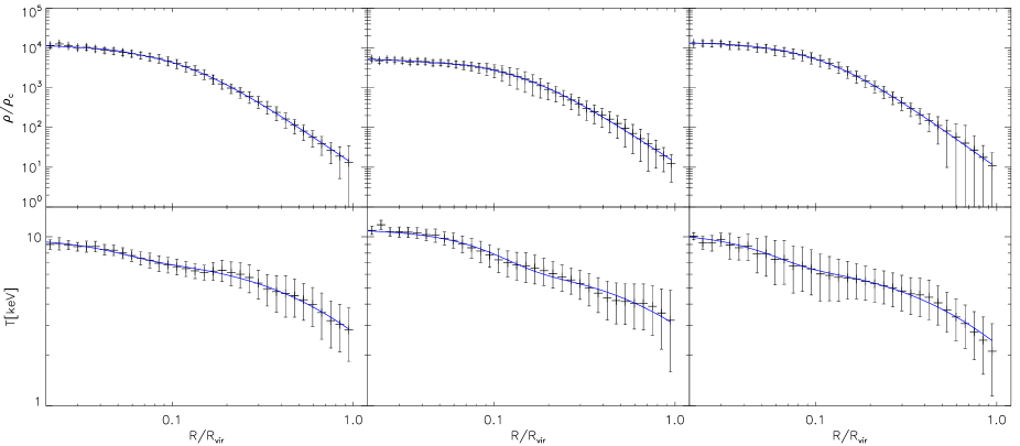
The resolutions (minimum AMR cell size) of the high-resolution simulations at $R$ = 0, 1 and 4$R_{\rm vir}$ were about 25 kpc, 80 kpc and 250 kpc. The total virial masses of the 10 massive clusters in our cluster sample fell between 1 and $2\times 10^{15}~{}{\mbox{\rm M}_{\odot}}$. Relaxed clusters were selected based on their density distribution: after the removal of filaments, we chose clusters with a smooth spherically averaged density profile with little angular variation, no sign of recent major merger events, and a relaxed core (for more details about our simulated cluster sample and analysis see Molnar et al. 2009). Out of a total of 10 clusters, two clusters satisfy our criteria for relaxed clusters (CL1 and CL2). We show spherically averaged gas density and temperature profiles for our massive relaxed clusters and one massive cluster with a non-relaxed core, CL3, in Figure 1. We include CL3 to check if we could constrain the large scale distribution of the ICG in a cluster which has a non-relaxed core, but is otherwise relaxed. The error bars represent the ${\it rms}$ of the density and temperature variations due to spherical averaging. While the density distributions are similar in all relaxed clusters, showing only small deviations from radial averaging, the temperature profiles show more variation. This is due to the sensitivity of the temperature to shocks from merging and internal flows. The solid curves in Figure 1 show the density and temperature profiles of the best-fit models for all simulated clusters (see below). The physical parameters of our selected clusters are summarized in Table 1.

We use spherically symmetric double $\beta$ models truncated at the virial radius, $R_{\rm vir}$, to describe the density distribution of the ICG in massive relaxed clusters. We use the same functional form for the temperature distribution at large radii as Loken et al. (2002), and a gaussian to describe the core region. The gas density and temperature models for massive clusters within the virial radius can be summarized as:

$$\rho(r) = \rho_{1}\theta_{1}(1+r^{\,2}/r^{\,2}_{1})^{-3\beta_{1}/2}+\rho_{2}\,\theta_{2}(1+r^{\,2}/r^{\,2}_{\rm core})^{-3\beta/2}$$ (1)

$$= \rho_{1}\,{\cal F}_{1}+\rho_{2}\,{\cal F}_{2}$$

and

$$T(r)=T_{0}\bigl{(}a_{c}\exp[-r^{2}/r_{c}^{2}]+1\bigr{)}\bigl{(}1+r/r_{\rm T}\bigr{)}^{-\delta},$$ (2)

where the large scale distribution is described by $r_{\rm core}$, $\beta$, $r_{\rm T}$ and $\delta$, and a possible extra component at the center is parameterized by $r_{1}$, $\beta_{1}$, $a_{\rm c}$ and $r_{\rm c}$, $\rho_{1}$ and $\rho_{2}$ are the central densities, and the transition between the two $\beta$ models at $a_{1}$ is facilitated by $\theta_{1}(r,a_{1})=\theta(a_{1}-r)$ and $\theta_{2}(r,a_{1})=\theta(r-a_{1})$, where $\theta$ is the Heaviside step function. We determine the best-fit parameters for each cluster by maximizing the likelihood functions

$$-2\,\ln{\cal L}_{F}=\sum_{i}{[(F_{O})_{i}-(F_{M})_{i}\}]^{2}\over\sigma_{Fi}^{2}}=\chi_{F}^{2},$$ (3)

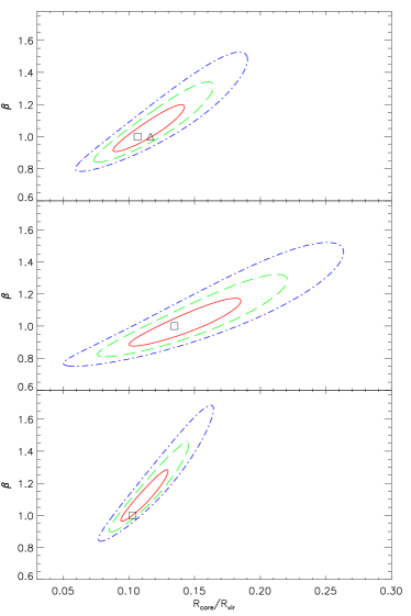
where $(F_{O})_{i}$ is the median value of the 3-dimensional (3D) density or temperature ($F=\rho$ or $T$) of a simulated cluster in the $i$-th radial bin, $(F_{M})_{i}$ is the corresponding value predicted by the model considered, and $\sigma_{Fi}$ is the corresponding standard deviation (here we use an approximation and assume that the sum of the fluctuations due to substructure, asphericity, etc. are gaussian, which is a reasonable assumption since we excluded filaments with large positive density fluctuations). These functions provide good fits to the density and temperature profiles of our selected clusters out to the virial radius: the fits are well within the 1$\sigma$ error bars due to spherical averaging, except for one point where the deviation is 1$\sigma$ for a temperature profile (see solid lines in Figure 1). The best fit parameters are summarized in Table 1. In Figure 2 we show the likelihood contours as a function of $r_{\rm core}$ and $\beta$ (the shape parameters of the second $\beta$ model, which describe the large scale distribution of the ICG) to the 3D distribution of the density in the outer parts of our selected clusters (the other parameters marginalized). The contour levels were determined based on the standard $\chi^{2}$ statistic. The likelihood contours show how well constrained the parameters are, subject to our assumption of spherical symmetry, and allow us to estimate the level of degeneracies between parameters. In carrying out fits to the 3D temperature distribution of simulated relaxed clusters we noticed that the exponent of the temperature model, $\delta$, does not change much from cluster to cluster (in agreement with an analysis using more clusters by Loken et al. 2002). Also, the best-fit models are not significantly better than models with fixed $\delta=1.6$. Thus we fix $\delta=1.6$ in our fitting and in the rest of our analysis. Since the best fit $\beta$ values are close to 1 in all selected clusters, we conclude that ICG models with $\beta=1$ and $\delta=1.6$ provide good fits to these clusters including CL3, which has a non-relaxed core. This result verifies our assumption that the outer region of CL3 is relaxed. Therefore, we find that the density distribution at large radii can be approximated with a power law, $r^{-\alpha}$, with $\alpha=3$, which is close to $\alpha=3.4$ as found by Roncarelli et al. (2006). Our results suggest that the pressure ($\propto\rho\,T$), at large radii can be approximated with a power law with $\alpha=3\beta+\delta=4.6$, which is close to $\alpha=5$, found by Nagai et al. (2007) and used by Mroczkowski et al. (2009). We conclude that the density and temperature functions (Equations 1 and 2) are adequate for relaxed clusters and provide a family of ICG models that can be fitted to observational data.

Table 1 Fitted shape parameters to clusters of galaxies from AMR simulations

ID	$M_{\rm vir}$	$R_{\rm vir}$	$a_{1}$	$r_{1}$	$\beta_{1}$	$r_{\rm core}$	$\beta$	$a_{\rm c}$	$r_{\rm c}$	$r_{\rm T}$	$\delta$
CL1	9.1E+14	2.0	0.05	0.013	0.10	0.113	1.033	0.26	0.052	1.07	1.6
CL2	1.2E+15	2.2	0.08	0.025	0.13	0.139	1.001	0.57	0.011	1.40	1.6
CL3	1.1E+15	2.1	–	–	–	0.110	1.096	0.46	0.056	1.00	1.6

X-ray observations of clusters of galaxies show that most relaxed clusters have cool cores (e.g., Vikhlinin et al. 2006), suggesting that cool-core clusters are relaxed. Cosmological numerical simulations suggest that early major mergers destroy the developing cool cores, but cool cores are strong enough to survive late major mergers, and thus cool cores are associated with cluster formation history and not necessarily with the dynamical state of clusters (Burns et al. 2008). This conclusion seems to be supported by the observational result that a substantial number of relaxed clusters do not posses a cool core at their center (e.g., HIFLUGS sample ). In our sample of clusters we do not have cool core clusters, but our method would work with either cool-core or non-cool-core clusters since we model the core of the cluster separately. In the case of cool-core clusters the amplitudes of our central temperature model, $a_{c}$, would be negative. Since outside of core gravitational physics dominates (Roncarelli et al. 2006), and the core region is modeled separately, we conclude that our adiabatic cosmological simulations and cluster models are adequate for our purpose.

4. SZ and X-ray Images of Simulated Clusters

We derive the 2-dimensional SZ and X-ray surface brightness distributions for simulated clusters in projections along the X, Y and Z axes (projections to the YZ, XZ and XY planes, Projection X, Y and Z, hereafter). We ignore relativistic effects, which is a good approximation in our case since the intra-cluster gas temperatures in our relaxed AMR clusters is less than about 10 keV. We derive the SZ signal in Projection Z by integrating along the LOS ($\ell$ which coincides with $z$ in this case) over the extent of the cluster (from $\ell_{1}$ to $\ell_{2}$) using

$$\Delta T_{CL}(x,y)=\Delta T_{CL0}\,N_{CLSZ}^{-1}\,\int_{\ell_{1}}^{\ell_{2}}n_{e}(x,y,\ell)\,T_{e}(x,y,\ell)\,d\ell,$$ (4)

where $x$ and $y$ are spatial coordinates in the plane of the sky, i.e. perpendicular to $\ell$; $n_{e}=f_{g}\rho_{g}/\mu_{e}m_{P}$ is the electron density, where $\mu_{e}$ is the mean molecular weight per electron and $m_{P}$ is the proton mass; $\rho_{g}$ is the gas density; $f_{g}$ is the mass fraction of baryons in the cluster that are contained in the ICG (we adopt $f_{g}=0.9$), and we use the standard assumption that the electron temperature equals the gas temperature, $T_{e}=T$. The frequency dependence is contained in $\Delta T_{CL0}=p(x_{\nu})\,{T_{\rm CMB}}\,k_{B}\sigma_{T}/(m_{e}c^{2})$, where the dimensionless frequency $x_{\,\nu}=h_{P}\nu/({k_{\rm B}}{T_{\rm CMB}})$, where $T_{\rm CMB}$ is the monopole term of the CMB, $h_{P}$ and $k_{B}$ are the constants of Planck and Boltzmann, and the function $p(x_{\nu})=x_{\nu}\coth(x_{\nu}/2)-4$ (e.g., Birkinshaw 1999). The SZ normalization is

$$N_{CLSZ}=\int_{\ell_{1}}^{\ell_{2}}n_{e}(0,0,\ell)\,T_{e}(0,0,\ell)\,d\ell.$$ (5)

In practice, we pixelize $x,y$ and $\ell$, and approximate the integral with a sum over the LOS from $\ell_{1}=-10$ Mpc to $\ell_{2}=10$ Mpc. Similar expressions were used for Projections X and Y.

Liu et al. (2010) studied the contamination from CMB, galactic diffuse emission and point sources in six clusters of galaxies observed in the first year of AMIBA. They found that the contamination is dominated by CMB fluctuations. The low level of contamination by point sources at around 90 GHz is due to the low angular resolution of AMIBA and the falling spectra of most radio sources. Even though some sources have inverted spectra, theoretical predictions based on VLA observations at lower frequencies suggest that only about 2% of clusters are contaminated at a significant level by point sources at this frequency (see Figure 13 of Sehgal et al. 2010). Therefore we include CMB contamination in our SZ image simulations but not point sources, since we can select relaxed clusters with no significant point source contamination for structural studies. Thus we have

$$\Delta T(x,y)=\Delta T_{CL}(x,y)+\Delta T_{CMB}(x,y),$$ (6)

where the CMB contamination, $\Delta T_{CMB}$, is generated as in Umetsu et al. (2004).

We derive the X-ray surface brightness in Projection Z by integrating along the LOS ($\ell$) over the extent of the cluster (from $\ell_{1}$ to $\ell_{2}$) as

$$S_{CL}(x,y)=S_{CL0}\,N_{CLX}\,\int_{\ell_{1}}^{\ell_{2}}n_{e}^{2}(x,y,\ell)\,T_{e}^{1/2}(x,y,\ell)\,d\ell,$$ (7)

where $S_{CL0}$ is the central X-ray surface brightness and the normalization, $N_{X}$, is

$$N^{\,-1}_{CLX}=\int_{\ell_{1}}^{\ell_{2}}n_{e}^{2}(0,0,\ell)\,T_{e}^{1/2}(0,0,\ell)\,d\ell,$$ (8)

where we use the scaling $S_{X}\propto\sqrt{T_{e}}$ for thermal bremsstrahlung (similar expressions were used for Projections X and Y). Similarly to the SZ surface brightness, we pixelize $x,y$ and $\ell$, and approximate the integral with a sum over the LOS from $\ell_{1}=-10$ Mpc to $\ell_{2}=10$ Mpc.

We simulate X-ray images of our relaxed AMR clusters assuming a field of view (FOV) of $16\arcmin\times 16\arcmin$ with a pixel size of $2\arcsec\times 2\arcsec$. We sample the Poisson distribution with expectation values equal to the integrated flux per pixel as

$$F_{X}(x,y)=F_{CL}(x,y)+B_{X},$$ (9)

where we calculate $F_{CL}(x,y)$ using Equation 7 assuming $F_{CL0}=7.5$ cnts/pixel ($S_{CL0}$ in units of integrated flux/pixel) and a uniform background of $B_{X}=0.2$ cnts/pixel (typical parameters for X-ray observations of clusters of galaxies).

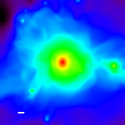
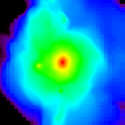
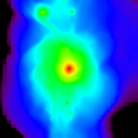
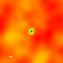
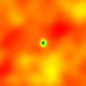
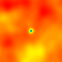
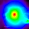
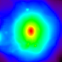
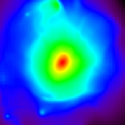
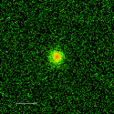
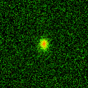
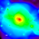
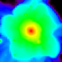
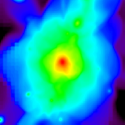
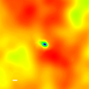
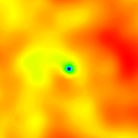
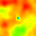
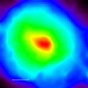
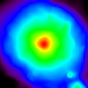
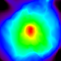
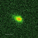
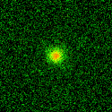
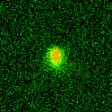
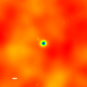
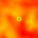
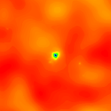
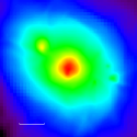
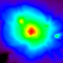
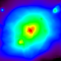
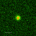
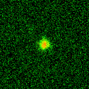
The Compton–$y$ images, $y=\int d\tau\,({k_{\rm B}}T_{e})/(m_{e}c^{2})$, where $\tau$ is the optical depth, the SZ images (cluster plus CMB at the AMiBA frequency band, 94 GHz), X-ray surface brightness, and simulated X-ray images including background noise, of our two relaxed clusters (CL1 and CL2) and one non-relaxed cluster (CL3) in Projections X, Y and Z assuming that they are located at a redshift of 0.3, are shown in Figures 3, 4 and 5. The Compton–$y$, X-ray surface brightness and simulated X-ray images are shown in logarithmic scale (first, third and fourth rows), and the SZ images with CMB contamination (second row) are shown in linear scale. The virial radii of our massive relaxed clusters are about 2 Mpc, which span about 8$\arcmin$ on the sky at this redshift. The dark blue regions ($\approx-1.2$ mK) on the SZ images mark the cluster centers, the yellow and red regions represent positive and negative CMB fluctuations with an amplitude of about $\pm 130\,\mu$K and an rms of about 90$\,\mu$K. In the Compton-$y$ images we can follow the diffuse gas out to about 3$R_{\rm vir}$, where the external shocks of massive clusters are found (see Molnar et al. 2009), but in the SZ images the diffuse gas around clusters seems to extend out to about $R_{\rm vir}$ only, due to contamination from CMB fluctuations, which dominate the large-scale structure. However, the SZ images of relaxed clusters, in most projections, show similar characteristics within the virial radius: a circularly-symmetric center and somewhat elongated outer regions. The core regions in the X-ray and SZ images (for example regions with yellow color in rows 1 and 3), in a few projections (Projection Z of CL1 and Projections X and Z of CL2), show asymmetry due to asphericity of the cluster and contamination by filaments in the LOS. The core region of non-relaxed cluster CL3 seems to be disturbed in all projections.

n

Figure 3.— Simulated images for Projections X, Y, and Z of relaxed cluster CL1 (left, middle and right column). From top to bottom: Compton-$y$, $\Delta T$ (including the cluster SZ signal and CMB fluctuations at 94 GHz), X-ray surface brightness and simulated X-ray image including background noise (logarithmic color scale except SZ map which is linear). The image size is $50^{\,\prime}\times 50^{\,\prime}$ for the SZ images (first two rows) and $16^{\,\prime}\times 16^{\,\prime}$ for the X-ray images (last two rows). The physical scale of 1 Mpc, same within each raw, is represented by horizontal bars.

Figure 4.— Same as Figure 3 but for simulated images of relaxed cluster CL2.

5.  Visibility Simulations

Interferometers measure visibilities, the Fourier transforms of the intensity distribution multiplied by the primary beam of the telescope. In the small-angle approximation, the visibilities can be written as

$$V_{\nu}(u,v)=\int^{\infty}_{-\infty}\int^{\infty}_{-\infty}B_{\nu}(x,y)\,I_{\nu}(x,y)\,e^{-i2\pi(ux+vy)}\,dx\,dy,$$ (10)

where $V_{\nu}(u,v)$ is the visibility function in the $uv$ plane, which is the Fourier conjugate of the positions, $x$ and $y$ on the sky. $B_{\nu}(x,y)$ and $I_{\nu}(x,y)$ are the primary telescope beam pattern and source intensity at $x$ and $y$ at frequency $\nu$, and we ignore effects due to a finite bandwidth, finite time averaging, and other effects associated with practical interferometers. We convert temperature differences to intensity units using

$${\Delta I\over{I_{\rm CMB}}}={x_{\,\nu}\,e^{\,x_{\nu}}\over(e^{\,x_{\nu}}-1)}\,{\Delta T\over{T_{\rm CMB}}},$$ (11)

where $I_{\rm CMB}$ is the intensity of the monopole term in the CMB. The visibilities, $V_{\rm CL}$ and $V_{\rm CMB}$ at frequency $\nu$ are calculated from $\Delta T_{\rm CMB}$ and $\Delta T_{\rm CL}$ using Equations 10 and 11.

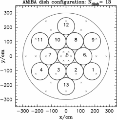
We simulated visibilities for mock two-patch  observations of our relaxed clusters assuming a compact configuration for the 13 antennas (Figure 6; for a detailed description see Koch et al., in preparation). In this configuration the many short baselines provide the highest sensitivity to the large-scale radio structure. The instrument noise and the contribution from the CMB were simulated in visibility space and added to the visibilities of the simulated clusters (see Umetsu et al. 2004). We assumed an observing time of 60 hours on-source. The errors in the azimuthally averaged visibilities for the simulated clusters, for the CMB and for the instrument noise are all comparable at this exposure time. Using longer exposure would reduce the errors for the instrument noise, but would not lower the errors either for our ICG models or for the CMB. Therefore we would not be able to reduce the error bars significantly by using longer observations. Usually a subtraction scheme is used in cluster SZ observation with half of the time on-source, and half of the time off source to reduce systematics, ground pick up and sky background (e.g., Wu et al. 2009). Therefore 60 hours of on-source integration involve 120 hour of total observing time. This can be conveniently accommodated into a 1-month observing schedule.

Figure 5.— Same as Figure 3 but for simulated images of cluster CL3.

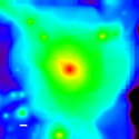
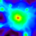
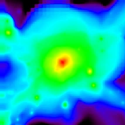
We use only projections of relaxed clusters which seem to show no contamination by filaments or distortion due to projection effects (Projections X and Y of CL1 and Projection Y of CL2), and a non-relaxed cluster, CL3, in a most relaxed projection, projection X. We derive simulated visibilities for two-patch observations as

$$V(u_{i},v_{i})=V_{source}(u_{i},v_{i})-V_{bkng}(u_{i},v_{i}),$$ (12)

where the on-source visibilities, $V_{\rm source}$, are

$${V_{\rm source}}(u_{i},v_{i})={V_{\rm CL}}(u_{i},v_{i})+{V_{\rm CMB}}(u_{i},v_{i})+{V_{\rm noise}}(u_{i},v_{i}),$$ (13)

and the off-source (background) visibilities, $V_{\rm bknd}$, are

$${V_{\rm bknd}}(u_{i},v_{i})={V^{\prime}_{\rm CMB}}(u_{i},v_{i})+{V^{\prime}_{\rm noise}}(u_{i},v_{i}),$$ (14)

where $V_{\rm SZ}$ is the visibility of the SZ signal, $V_{\rm CMB}$, $V_{\rm noise}$, and ${V^{\prime}_{\rm CMB}}$, ${V^{\prime}_{\rm noise}}$ are two sets of visibilities of the CMB fluctuations and noise (different for on- and off-source observations). We assumed that the CMB fluctuation fields for the two patches (about one degree apart) are uncorrelated, which is a conservative assumption: this way we somewhat overestimate the noise due to the CMB. Since our models are spherically symmetric, we have no constraints on them from the imaginary part of the model visibilities (the imaginary part is identically zero), therefore we work only with the real part of the visibilities. Note that in real applications the imaginary parts can be used to check the amplitude of the CMB fluctuations in the field, assess non-sphericity of the cluster and the pointing accuracy.

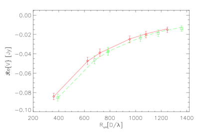
As an illustration, in Figure 7 we show the radial profile of the real part, ${\cal R}e(V)$, of the azimuthally averaged simulated visibilities of one realization of a two-patch observation for CL1 in Projection Y for the 90 and 98 GHz AMiBA channels (Channels A and B, Ho et al. 2009) as a function of $R_{uv}$. Since the length scale for the visibility data is in units of the observing wavelength, the visibilities are represented by two sets of curves. The red diamonds and green squares with error bars represent visibilities for Channel A and B. The error bars represent the rms of the azimuthally averaged real part of the visibilities at the  baselines. Visibilities of other projections of CL1 and projections of CL2 and CL3 with no contamination from filaments are very similar due to the structural similarity among the cluster SZ images in these projections (see Figures 3, 4 and 5).

6. Model Fitting

We use non-isothermal double $\beta$ models truncated at the virial radius to describe the ICG. We determine the best-fit parameters using likelihood functions. Our model for the SZ surface brightness distributions (Equations 1 and 2) has eleven free parameters: ten shape parameters, $p=(a_{1},r_{1},\beta_{1},{r_{\rm core}},\beta,a_{c},r_{c},{r_{\rm T}},\delta,R_{\rm vir})$, and one amplitude, $\Delta T_{0}$. Unfortunately, due to limited spatial resolution, FOV and receiver noise, we do not expect to be able to determine all ten parameters using . Thus, similarly to Mroczkowski et al. (2009), we reduce the number of free parameters in our models. We proceed the following way: first we determine the shape parameters for the central part of the cluster, $a_{1}$, $r_{1}$, $\beta_{1}$, $a_{c}$, $r_{c}$, and the core radius for the large scale distribution, $r_{\rm core}$ from simulated X-ray observations (fixing $\beta=1$, $r_{T}=1.0$ $R_{\rm vir}$ and $\delta=1.6$ based on our results from numerical simulations). We assume that the X-ray surface density and temperature are determined with acceptable accuracy only in the central part of the cluster, to 0.5$R_{\rm vir}$ and 0.2$R_{\rm vir}$. Therefore $r_{\rm T}$ cannot be determined from fits to the X-ray temperature profile, and the X-ray emissivity within 0.5$R_{\rm vir}$ gives no useful constraints on the large scale distribution of the temperature. Having determined the shape parameters for the central part, we derive constraints on the temperature scale parameter, $r_{\rm T}$, from simulated  visibilities.

Figure 6.— Antenna layout for  in the compact configuration (13 dishes with 1.2 m diameter) used for simulations in this paper. Other possible antenna positions are marked with $\times$-s.

We calculate the predicted integrated X-ray flux/pixel for our X-ray model as

$$F_{XM}=F_{CLM}+B_{XM},$$ (15)

where $F_{CLM}$ is our cluster model and $B_{XM}$ is the background. We calculate $F_{CLM}$ as

$$F_{CLM}(x,y,p)=F_{1}\,N_{X1}\,{\cal I}_{X1}(x,y,p)+F_{2}\,N_{X2}\,{\cal I}_{X2}(x,y,p),$$ (16)

where $F_{1}$ and $F_{2}$ are the central integrated flux/pixel for the two model components, the normalizations are $N_{X1}^{\;-1}={\cal I}_{X1}(0,0,p)$ and $N_{X2}^{\;-1}={\cal I}_{X2}(0,0,p)$, and

$${\cal I}_{X1}(x,y,p) = 2\,\int_{0}^{\ell_{c}}{\cal F}_{1}^{2}\,(1+r/r_{T})^{-\delta/2}d\ell$$

$${\cal I}_{X2}(x,y,p) = 2\,\int_{0}^{\ell_{c}}{\cal F}_{2}^{2}\,(1+r/r_{T})^{-\delta/2}d\ell,$$ (17)

where $r^{2}=x^{2}+y^{2}+\ell^{2}$, and the cut off in the LOS is $\ell^{2}_{c}=R_{\rm vir}^{2}-x^{2}-y^{2}$. We ignore the error in the X-ray background, $B_{XM}$ since it is negligible relative to other sources of error, such as, for example, errors due to azimuthal averaging.

We experimented with the likelihood ratio for Poisson distribution and Mighell’s $\chi_{\gamma}^{2}$ statistic (see Mighell 1999 for a detailed analysis) in fitting this structure. We found that the fitted parameters obtained by these two methods are virtually identical. Therefore we decided to use the Poisson likelihood ratio test:

$$-\ln{\cal L}_{X}=\sum_{i}M_{i}-N_{i}+N_{i}\,\ln(N_{i}/M_{i}),$$ (18)

where $N_{i}$ and $M_{i}$ are the observed and expected numbers of photons.

We derive spectroscopic-like X-ray temperature profiles, $T_{sp}$, for our simulated clusters using the weighting scheme of Mazzotta et al (2004), which has been shown to provide temperature profiles similar to those observed with Chandra and XMM (Nagai et al. 2007),

$$T_{sp}={\int w_{sp}\;TdV\over\int w_{sp}\;dV},$$ (19)

where the weight is $w_{sp}=n^{2}/T^{3/4}$. We determine the best fit parameters for the temperature model maximizing the likelihood function

$$-2\,\ln{\cal L}_{T}=\sum_{i}{[(T_{sp})_{i}-(T_{M})_{i}\}]^{2}\over\sigma_{i}^{2}},$$ (20)

where $(T_{sp})_{i}$ and $(T_{M})_{i}$ are the median values of the observed and model spectroscopic temperatures, and $\sigma_{i}$ is the standard deviation in the $i$th radial bin.

Figure 7.— Real part, ${\cal R}e\,\{V\}$ (in Jy), of the azimuthally averaged simulated visibilities as a function of $uv$ radius ($R_{uv}$) in Projection Y of the CL1 (plus CMB and noise, one realization) for  Channel A and B (red diamonds and green squares) in a compact configuration (see Figure 6). The error bars represent instrumental errors of 60 hour observations. The best-fit $\beta$ model is also shown for the two channels (red solid and green dashed lines).

Figure 8.— Radial profiles of X-ray surface brightness, gas temperature, normalized SZ surface brightness and gas density (top to bottom) in projections X and Y of CL1, projection Y of CL2 and projection X of CL3 (left to right columns). Blue plus signs and error bars: AMR cluster in projection (no noise, no CMB; first, second and 3rd rows); red squares: simulated data points for one realization including contamination; black plus signs and error bars: spherically averaged gas temperature and density distributions in simulated clusters based on their 3D distributions (shown out to the virial radius; second and 4th row); blue dashed lines: best fitted models to simulated X-ray and  observations (first, second and 3rd rows); blue solid lines: 3D distribution of the temperature and density in simulated clusters based on fits to the projected (2D) X-ray surface brightness, gas temperature, and SZ surface brightness profiles (second and 4th rows).

Since the shape parameters of the inner part of clusters, $r_{1}$, $\beta_{1}$, $r_{\rm core}$, $a_{c}$, and $r_{c}$, are not sensitive to the large-scale distribution of the temperature (heavily weighted towards the center of the cluster), we determine them fixing $\beta=1$, $r_{T}=1$ and $\delta=1.6$ (based on our results from fitting to the density and temperature distributions of our simulated clusters). In our case, since $\beta=1$, the X-ray emissivity, which is proportional to $(1+r^{2}/{r_{\rm core}}^{2})^{-3}$ in the outer parts of the cluster, drops about six orders of magnitude from the cluster center to the virial radius. Therefore a moderate change in $R_{\rm vir}$ (say 20%) causes only an insignificant change in the X-ray signal (Equation 6) due to a change in the upper limit, $\ell_{c}$ (except around $R_{\rm vir}$  where the X-ray signal is negligible; see Figures 3, 4 and 5). For our purposes, therefore, we fix the value of $R_{\rm vir}$ assuming that an estimate for its value with a 20% accuracy is available from other measurements. We determine the shape parameters, $r_{1}$, $\beta_{1}$, $r_{\rm core}$, $a_{c}$, and $r_{c}$ by maximizing the likelihood functions, Equations 18 and 20. In practice, since the spectroscopic-like temperature is not sensitive to a few tens of percent change in the $\beta$ model parameters, we can determine the shape parameters using iteration. We use the likelihood function for the X-ray emission (Equation 18) to determine $r_{1}$, $\beta_{1}$ and $r_{\rm core}$, and then the likelihood function for the X-ray temperature (Equation 20) to determine $a_{c}$, and $r_{c}$, then we iterate over these steps (usually only two steps are needed). This method proved to be faster than a search for the maximum likelihood in the five dimensional parameter space.

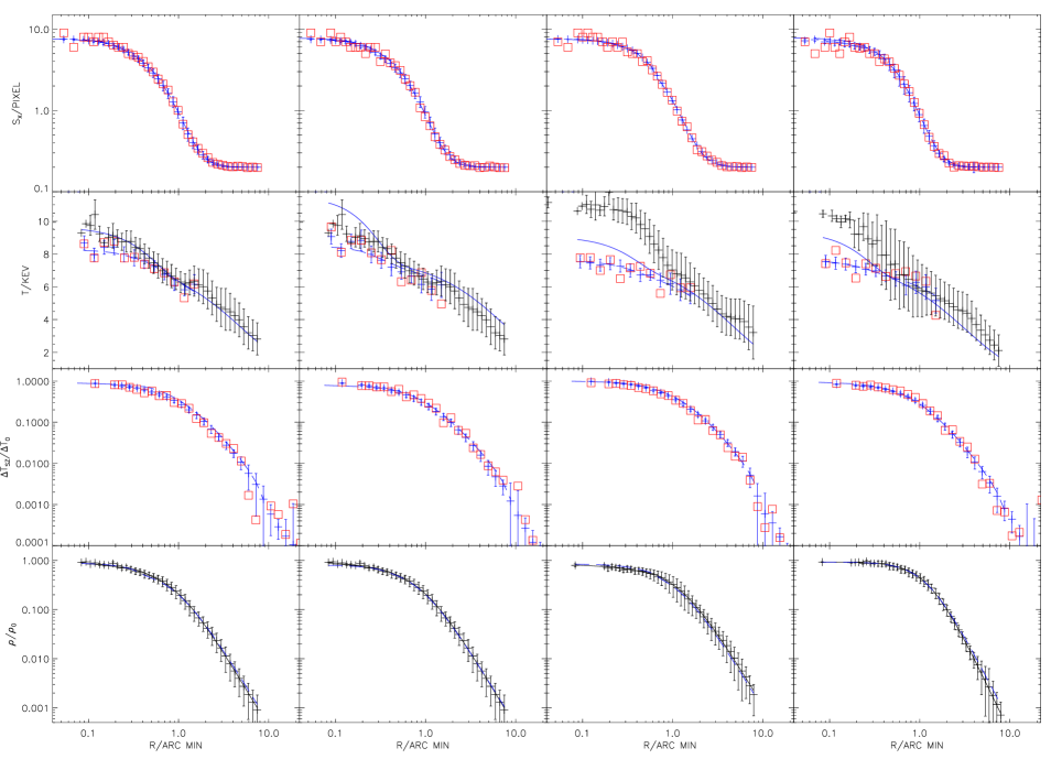
In Figure 8 we show the radial profiles of the X-ray surface brightness distribution, the spectroscopic temperature and the SZ signal for Projections X and Y of CL1, Projection Y of CL2, and Projection X of CL3 (blue plus signs with error bars representing dispersion in azimuthal averaging). For each projection, we also show one realization of our Monte Carlo simulations (red squares), and, for comparison, the temperature and density profiles derived from their respective 3D distributions (black plus signs with error bars representing dispersion in spherical averaging, solid black lines represent best fit models; same as in Figure 1). We also show the best fit X-ray surface brightness models (blue dashed lines) derived as described in the previous paragraph. The other dashed and solid blue lines, explained later in this section, are included here for later convenience. Based on the first row in this figure, we conclude that our non-isothermal double $\beta$ models provide good fits to the X-ray surface brightness profiles in our relaxed clusters (CL1 and CL2), and even in our cluster with a non-relaxed core (CL3).

The best fit core radii of the outer $\beta$ model from fitting our non-isothermal double $\beta$ models to the X-ray surface brightness distributions and temperature profiles (with $\beta=1$ fixed) in different projections are shown in Figure 2 (squares and triangles). These values are within the 68% CL of the best fit values obtained from fitting double $\beta$ models directly to the 3D distribution of the density (solid red lines). We conclude that the core radius for the large scale distribution can be determined accurately, with no bias, from X-ray data using our ICG models.

Figure 9.— Likelihood contours (68%, 95.4% and 99.7% CLs, solid red, dashed green, and dash-dotted blue lines) for fitting for the normalized SZ amplitude ($\Delta T_{0}/\Delta T_{0b}$) and the temperature scale radius $r_{T}$ in projections X and Y of CL1, projection Y of CL2 and projection X of CL3 (from top to bottom).

As a second and final step, we calculate the visibilities for our models, $V_{M}$, at frequency $\nu$, using Equations 10 and 11, as

$$\Delta T_{CLM}(x,y)=\Delta T_{0}\,N_{SZ}\,{\cal I}_{SZ}\,(x,y,p),$$ (21)

where $\Delta T_{0}$ is the central SZ amplitude, the normalization is $N^{\,-1}_{SZ}={\cal I}_{SZ}(0,0,p)$, and

$${\cal I}_{SZ}(x,y,p)=2\,\int_{0}^{\ell_{c}}{\rho_{1}\,{\cal F}_{1}+\rho_{2}\,{\cal F}_{2}\over\rho_{1}+\rho_{2}}\,(1+r/r_{T})^{-\delta}d\ell.$$ (22)

Note, that since $r/r_{\rm core}$ and $r/r_{T}$ are both dimensionless, $\Delta T_{CLM}(x,y)$ depends on $R_{\rm vir}$ only through $\ell_{c}$. We use Equation 12 to derive simulated observed visibilities, $V_{O}$, for each realization as described in Section §5.

We determine the best fit parameters for our models by maximizing the SZ likelihood function defined as

$$-2\,\ln{\cal L}_{SZ}=\sum_{i,j}{[{\cal R}e\{V_{O}(R_{uv}^{\,i};\nu_{j})\}-{\cal R}e\{V_{M}(R_{uv}^{\,i};\nu_{j})\}]^{2}\over\sigma_{ij}^{2}},$$ (23)

where ${\cal R}e\{V_{O}\}$ and ${\cal R}e\{V_{M}\}$ are the azimuthally averaged real part of the observed and model visibilities at the $i$th $uv$ radius, $R_{uv}^{\,i}$, at frequency $\nu_{j}$, where $j=1,2$ for the two AMiBA frequency channels, and $\sigma_{ij}$ is the Gaussian noise, which is assumed to be the same for all antenna pairs and frequencies.

Similarly to the X-ray signal, a moderate change in $R_{\rm vir}$ (all the other parameters fixed) causes only an insignificant change in the SZ signal (Equation 22) because the pressure is about four orders of magnitude smaller at the virial radius than at the center of the cluster. In this final step, we assumed that we determined the model parameters for the central region of clusters ($r_{1}$, $\beta_{1}$, $a_{c}$, $r_{c}$) and $r_{\rm core}$ from fitting our models to the X-ray surface brightness and temperature distribution (as above), therefore, among the shape parameters of our non-isothermal double $\beta$ models, $p=(r_{1},\beta_{1},{r_{\rm core}},1,a_{c},r_{c},{r_{\rm T}},1.6,R_{\rm vir})$, there is only one unknown parameter, $r_{\rm T}$. We determine the best fit for $r_{\rm T}$ and the normalized SZ amplitude ($\Delta T_{SZ}/\Delta T_{0}$) by maximizing the SZ likelihood function, Equation 23.

In Figure 8 we show the 2D projected temperature and SZ profiles for the best fits (dashed blue lines, 2nd and 3rd row). Solid blue lines represent the 3D best fit radial profiles for the temperature and density (2nd and 4th row). In some cases the deprojected temperature profiles are underestimated by 10–20% close to the cluster center because cold substructures in the LOS reduce the spectroscopic temperature and the weighting suggested by Mazzotta et al (2004) does not always correct for this effect accurately. However, these deviations in the central temperature do not affect the fits to the large scale SZ profiles as observed by  because of the low resolution of the instrument.

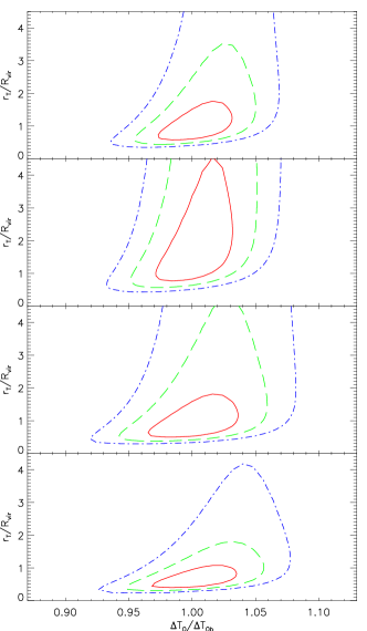
In Figure 9 we show the CLs for the temperature scale radius $r_{T}$ and the normalized SZ amplitude in different projections of X and Y of CL1, Projection Y of CL2 and Projection X of CL3. The normalization, $\Delta T_{0}/\Delta T_{0b}$, is the ratio of the best-fit $\Delta T_{0}$ for each Monte Carlo simulation to the best-fit value determined from all Monte Carlo simulations. The confidence levels have been determined using Monte Carlo simulations. The contours for the 68% CL, for example, are the smoothed version of the contours containing 68% of the simulated best fit points based on simulations.

7. Discussion

We have simulated  observations of massive relaxed clusters of galaxies including CMB contamination and receiver noise using clusters drawn from cosmological numerical simulations to assess how well we should be able to constrain the large-scale distribution of the ICG. Our simulated SZ images (rows 2 in Figures 3, 4 and 5) show that at 94 GHz, on the scale of the cluster cores (few arc minutes), the cluster SZ signal dominates the CMB fluctuations, so that CMB contamination is not important in surveys searching for rich clusters. On a scale of ten arc minutes, corresponding to the extent of the ICG in massive clusters at $z\approx 0.3$, the CMB contamination is at a comparable level to the SZ signal. Contamination from CMB fluctuations is also important in the regions in galaxy clusters close to their virial radius. Spectral separation of the cluster SZ and the CMB signals based on multi-frequency observations seems to be essential for studying the outskirts of galaxy clusters and the SZ signature of the large-scale structure.

Using our AMR simulations, we showed that a spherical non-isothermal double $\beta$ model with a temperature distribution described by Equation 2 provides good fits to the radial distributions of the ICG in our selected massive clusters. We generated X-ray and SZ images of our clusters drawn from numerical simulations assuming that the clusters are at a redshift of 0.3.

We used the simulated X-ray data to determine the shape parameters, $r_{1}$, $\beta_{1}$, $r_{\rm core}$, of the double $\beta$ model for the density distribution and the central model parameters, $a_{c}$ and $r_{c}$ of the temperature model by minimizing the likelihood functions Equations 18 and 20. We assumed that $R_{\rm vir}$ is constrained to $\pm 20$% by other measurements, for example, from gravitational lensing, as done by Broadhurst and Barkana (2008) and Umetsu et al. (2009). This is a conservative estimate since combining weak and strong lensing data, one can determine $R_{\rm vir}$ with about 5% accuracy (Umetsu et al., 2010). The values of the likelihood functions corresponding to the 68%, 95.4% and 99.7% CLs for fitting for $r_{\rm core}$ and $\beta$ to the 3D density distribution of simulated clusters are shown in Figure 2. The elongated shape of the confidence levels in this figure shows a degeneracy between the two shape parameters of the $\beta$ model: $r_{\rm core}$ and $\beta$. Combinations of small ($r_{core},\beta$) or large ($r_{core},\beta$) both give good fits to the density distributions. A similar degeneracy has been reported for fitting $\beta$ models to X-ray observations (e.g., Grego et al. 2001; Reese et al. 2000; Birkinshaw & Hughes 1994).

As a final step, we used simulated  visibilities to determine the temperature scale radius, $r_{\rm T}$, and the SZ normalization (fixing all other parameters) by maximizing the SZ likelihood function, ${\cal L}_{SZ}$ (Equation 23). Our results are shown in Figure 9. For model fits to Projections X and Y of CL1, we obtain $r_{T}=1.023_{-0.4}^{+0.5}$ $R_{\rm vir}$, and $r_{T}=1.60_{-0.5}^{+4.0}$ $R_{\rm vir}$. Fits to Projection Y of CL2 yield $r_{T}=0.927_{-0.4}^{+0.5}$ $R_{\rm vir}$. We obtain $r_{T}=0.631_{-0.2}^{+0.3}$ $R_{\rm vir}$ for our cluster with a non-relaxed core, CL3, in Projection X.

All results for the temperature scale radius, $r_{\rm T}$, are within 68% of the best-fit values based on fitting the 3D distributions (Table 1). The 68% CLs for all clusters with circular projected X-ray distribution (Projection X of CL1 and Projection Y of CL2) and the cluster with a non-relaxed core (Projection X of CL3) are within 50% of the best fit values. Therefore our results suggest that, using relaxed clusters with circular morphology, we should be able to use  along with X-ray observations to obtain unbiased parameters for our non-isothermal double $\beta$ models (even for clusters with a non-relaxed core, such as CL3), and constrain $r_{\rm T}$ within 50%. Our model fits to Projection Y of CL1, a relaxed cluster with elliptical morphology, although returning $r_{\rm T}$ within 68% of the 3D fitted value, shows a large error due to asphericity. We expect that using a more accurate elliptical model would result in better constraints on $r_{\rm T}$. The SZ amplitude, which is important for the determination of the Hubble constant for example, can be determined with 3-4%, which is better than the expected accuracy of the absolute calibration of .

We carried out simulations at different redshifts between 0.1 and 0.4. For a distant cluster the beam dilution reduces the signal; if the cluster is too close, the outer parts of the cluster fall outside of the FOV. We have found that the optimal redshift for determining the large-scale distribution of the ICG with  is $z\approx 0.3$.

We conclude that we should be able to use  to determine the large-scale distribution of the ICG in massive relaxed clusters of galaxies located at a redshift of 0.3 by determining the temperature scale radius with an about 50% statistical accuracy. AMiBA, as upgraded to 13 dishes with 1.2-m in diameter, will be a powerful tool for constraining the large-scale distribution of the ICG.

The degeneracy between density and X-ray temperature can be broken and determined out to the virial radius using current X-ray telescopes. However, an accurate determination of the temperature profile out to $R_{\rm vir}$ requires a long exposure time (due to the low photon count rates at the outer parts of clusters) and mosaicing (due to the limited FOV). This is the reason why only a few attempts have been carried out to map the outer regions of clusters (see §2). Constraints on the large scale distribution of the ICG similar to AMIBA can be derived using bolometer cameras. In principle, bolometer cameras with arc minute resolution can cover clusters with the necessary sensitivity out to $R_{\rm vir}$ (ACT: Hinks et al. 2009; SPT: Plagge et al. 2009), although this has not yet been done.

In this paper we considered spherically symmetric galaxy cluster models, and focused on statistical errors due to the  telescope and receiver system. We should be able to reduce the observation time needed to measure $r_{\rm T}$ by using a more sophisticated observational strategy. A single pointing to the center of the cluster, although it simplifies the data analysis, has the disadvantage that it has a reduced sensitivity at the outer parts of the cluster, where the signal is weaker. We expect that mosaic observations including pointings towards the outer regions in clusters, although more difficult to analyze, would enable us to reach our goal with an exposure time shorter than 60 hrs. We leave simulations to quantify the effects of mosaic observations and more sophisticated ICG models on parameter determination for future work, as well as a detailed study of parameter estimation from a large set of simulated relaxed clusters with a wider range of mass and redshift.

References

- Allen et al. (2004) Allen, S. W., Schmidt, R. W., Ebeling, H., Fabian, A. C., & van Speybroeck, L. 2004, MNRAS, 353, 457
- Afshordi et al. (2007) Afshordi, N, Lin, Y. T., Nagai, D., & Sanderson, A. J. R. 2007, MNRAS, 378, 293
- Atrio-Barandela et al. (2008) Atrio-Barandela, F., Kashlinsky, A., Kocevski, D., & Ebeling, H. 2008, ApJ, 675, L57
- Bautz et al. (2009) Bautz, M. W., et al. 2009, PASJ, 61, 1117
- Birkinshaw (1999) Birkinshaw, M. 1999, Phys. Rept., 310, 97
- Birkinshaw & Hughes (1994) Birkinshaw, M., & Hughes, J. P. 1994, ApJ, 420, 33
- Borgani (2006) Borgani, S. 2006, arXiv:0605575
- Broadhurst & Barkana (2008) Broadhurst, T. J., & Barkana, R. 2008, MNRAS, 390, 1647
- Bryan & Norman (1998) Bryan, G.L., & Norman, M.L. 1998, ApJ, 495, 80
- Burns et al. (2008) Burns, J. O., Hallman, E. J., Gantner, B., Motl, P. M., & Norman, M. L. 2008, ApJ, 675, 1125
- Carlstrom et al. (2002) Carlstrom, J. E., Holder, G. P., & Reese, E. D. 2002, ARA&A, 40, 643
- Cavaliere & Fusco-Femiano (1976) Cavaliere, A., & Fusco-Femiano, R., 1976, A&A, 49, 137
- Chen et al. (2009) Chen, M.-T., et al. 2009, ApJ, 694, 1664
- Dunkley et al. (2009) Dunkley, J., et al. 2009, ApJS, 180, 306
- Ettori (2004) Ettori, S. 2004, Ap&SS, 290, 177
- Ettori & Balestra (2009) Ettori, S. & Balestra, I. 2009, A&A, 496, 343
- Fang & Haiman (2008) Fang, W., & Haiman, Z. 2008, ApJ, 680, 200
- Grego et al. (2001) Grego, L., Carlstrom, J. E., Reese, E. D., Holder, G. P., Holzapfel, W. L., Joy, M. K., Mohr, J. J., & Patel, S. 2001, ApJ, 552, 2
- Haiman et al. (2001) Haiman, Z., Mohr, J. J., & Holder, G. P. 2001, ApJ, 553, 545
- Hallman et al. (2007) Hallman, E. J., Burns, J. O., Motl, P. M., & Norman, M. L. 2007, ApJ, 665, 911
- Haugbolle et al. (2007) Haugbolle, T., Sommer-Larsen, J., & Pedersen, K., 2007, arXiv:0712.2453v1
- Henry (2000) Henry J. P. 2000, ApJ, 534, 565
- Hincks et al. (2009) Hinks, A. D., et al., 2009, arXiv:0907.0461
- Ho et al. (2009) Ho, P. T. P., et al. 2009, ApJ, 694, 1610
- Holder, Haiman & Mohr (2001) Holder, G., Haiman, Z., & Mohr, J. J. 2001, ApJ, 560, L111
- Huang et al. (2010) Huang, C.-W. L., et al. 2010, ApJ, 716, 758
- Kawahara et al. (2008) Kawahara, H., Kitayama, T., Sasaki, S., & Suto, Y. 2008, ApJ, 674, 11
- Koch et al. (2009) Koch, P. M., et al. 2009, ApJ, 694, 1670
- Koch et al. (2010) Koch, P. M., et al. 2010, ApJ, submitted
- Lin et al. (2009) Lin, K.-Y., et al. 2009, ApJ, 694, 1629
- Liu et al. (2009) Liu, G. C., et al. 2009, ApJ, submitted
- Loken et al. (2002) Loken, C., Norman, M. L., Nelson, E., Burns, J., Bryan, G. L., & Motl, P. 2002, ApJ, 579, 571
- Mazzotta et al. (2002) Mazzotta P., Rasia E., Moscardini L., & Tormen G., 2004, MNRAS, 354, 10
- Maughan et al. (2008) Maughan, B. J., Jones, C., Forman, W., & Van Speybroeck, L. 2008, ApJS, 174, 117
- Mighell (2009) Mighell, K., J., 1999, ApJ, 518, 380
- Molnar, Birkinshaw & Mushotzky (2002) Molnar, S. M., Birkinshaw, M., & Mushotzky, R. F. 2002, ApJ, 570, 1
- Molnar et al. (2004) Molnar, S. M., Haiman, Z., Birkinshaw, M., & Mushotzky, R. F. 2004, ApJ, 601, 22
- Molnar et al. (2009) Molnar, S. M., Hearn, N., Haiman, Z., Bryan, G., Evrard, A., & Lake, G. 2009, ApJ, 696, 1640
- Mroczkowski et al. (2009) Mroczkowski, T., et al. 2009, ApJ, 694, 1034
- Muchovej et al. (2007) Muchovej, S., et al. 2007, ApJ, 663, 708
- Nagai et al. (2007) Nagai, D., Kravtsov, A. V., & Vikhlinin, A. 2007, ApJ, 668, 1
- Nishioka et al. (2009) Nishioka, H., et al. 2009, ApJ, 694, 1637
- O’Shea et al. (2004) O’Shea, B.W., Bryan, G. L., Bordner, J., Norman, M. L., Abel, T., Harkness, R., & Kritsuk, A. 2004, arXiv:0403044
- Plagge et al. (2009) Plage, T., et al., 2009, arXiv:0911.2444
- Reese et al. (2000) Reese, E. D., et al. 2000, ApJ, 533, 38
- Rephaeli (1995) Rephaeli, Y. 1995, ARA&A, 33, 541
- Roncarelli et al. (2006) Roncarelli, M., Ettori, S., Dolag, K., Moscardini, L., Borgani, S., & Murante, G. 2006, MNRAS, 373, 1339
- Sarazin (1988) Sarazin, C. L., 1988, Cambridge Astrophysics Series, Cambridge: Cambridge University Press, 1988
- Sehgal et al. (2010) Sehgal, N., Bode, P., Das, S., Hernandez-Monteagudo, C., Huffenberger, K., Lin, Y.-T., Ostriker, J. P., & Trac, H. 2010, ApJ, 709, 920
- Sunyaev & Zel’dovich (1980) Sunyaev, R. A., & Zel’dovich, Ya. B. 1980, ARA&A, 18, 537
- Umetsu et al. (2004) Umetsu, K., Chiueh, T., Lin, K.-Y., Wu, J.-M., & Tseng, Y.-H. 2004, Modern Physics Letters A, 19, 1027 (arXiv:0402009)
- Umetsu et al. (2009) Umetsu, K., et al. 2009, ApJ, 694, 1643
- Umetsu et al. (2010) Umetsu, K., Medezinski, E., Broadhurst, T., Zitrin, A., Okabe, N., Hsieh, B.-C., & Molnar, S. M. 2010, ApJ, 714, 1470
- Vikhlinin et al. (2005) Vikhlinin, A., Markevitch, M., Murray, S. S., Jones, C., Forman, W., & Van Speybroeck, L. 2005, ApJ, 628, 655
- Voit (2005) Voit, G. M. 2005, Reviews of Modern Physics, 77 207
- Vikhlinin et al. (2008) Vikhlinin, A., et al. 2008, arXiv:0812.2720
- Wu et al. (2009) Wu, J.-H. P., et al. 2009, ApJ, 694, 1619
- Younger & Bryan (2007) Younger, J. D., & Bryan, G. L. 2007, ApJ, 666, 647