Application of Bayesian model averaging to measurements of the primordial power spectrum

Abstract

Cosmological parameter uncertainties are often stated assuming a particular model, neglecting the model uncertainty, even when Bayesian model selection is unable to identify a conclusive best model. Bayesian model averaging is a method for assessing parameter uncertainties in situations where there is also uncertainty in the underlying model. We apply model averaging to the estimation of the parameters associated with the primordial power spectra of curvature and tensor perturbations. We use CosmoNest and MultiNest to compute the model evidences and posteriors, using cosmic microwave data from WMAP, ACBAR, BOOMERanG and CBI, plus large-scale structure data from the SDSS DR7. We find that the model-averaged 95% credible interval for the spectral index using all of the data is $0.940<n_{\rm s}<1.000$, where $n_{\rm s}$ is specified at a pivot scale $0.015\,{\rm Mpc}^{-1}$. For the tensors model averaging can tighten the credible upper limit, depending on prior assumptions.

I Introduction

Measurements of the cosmic microwave background (CMB) by the Wilkinson Microwave Anisotropy Probe (WMAP) have, over the last few years wmap3 ; wmap5 ; wmap7 , produced ever more refined constraints on the cosmological parameters, particularly those relating to the spectrum of primordial perturbations. Typically, when constraints are quoted this is done under the assumption that a particular underlying model is the correct one, but there remains some uncertainty as to which is the most appropriate model to fit to the data. One approach to this is model selection, which asks the data to rank the models under consideration, but current applications MPL ; PML ; RT2007 ; PPS_ev ; Kawasaki:2009 ; Kilbinger:2009 indicate that several models are still allowed.

Such uncertainty in the correct choice of model can be handled by the technique of Bayesian model averaging hoeting , which allows one to assess parameter uncertainties in the presence of model uncertainty. The individual posteriors from different models will contribute to the model-averaged posterior, weighted by their model likelihood. Our aim in this paper is to apply this technique to measurements of the primordial spectrum. In Section II we review the Bayesian ideas we are applying to measurements of the primordial power spectrum. In Section III we carry out the analysis.

II Multi-model Bayesian statistics

Bayes’ theorem states the relationship between models ($\mathcal{M}$), parameters ($\bar{\theta}$) and data ($D$)

$$P(\bar{\theta}|D,\mathcal{M})=\frac{P(D|\bar{\theta},\mathcal{M})P(\bar{\theta}|\mathcal{M})}{P(D|\mathcal{M})}\,,$$ (1)

where $P(\bar{\theta}|\mathcal{M})$ is the prior probability distribution of the parameters (assuming some model), $P(D|\bar{\theta},\mathcal{M})$ is the likelihood, and $P(\bar{\theta}|D,\mathcal{M})$ is the posterior probability distribution of the parameters. The prior is updated to the posterior by the likelihood. The term $P(D|\mathcal{M})$ represents the model likelihood, and is called the evidence. In the case of single-model inference (where only a single model or set of parameters is considered), the evidence is simply a normalizing constant, set to satisfy the condition that the posterior distribution sums to unity.

However, in most interesting cases in cosmology, the correct model is not known, and the evidence takes different values for different models. We can use Bayes’ theorem again, at one level above, to calculate the posterior odds between different models and perform model selection,

$$\frac{P(\mathcal{M}_{1}|D)}{P(\mathcal{M}_{2}|D)}=\frac{P(D|\mathcal{M}_{1})}{P(D|\mathcal{M}_{2})}\frac{P(\mathcal{M}_{1})}{P(\mathcal{M}_{2})}\,.$$ (2)

Here $\mathcal{M}_{1}$ and $\mathcal{M}_{2}$ are the different models under consideration, $P(\mathcal{M}_{i})$ gives the prior probability of each model, and $P(\mathcal{M}_{i}|D)$ is the model posterior probability. Thus the model posterior probability is updated from the prior by the evidence. If the model priors are equal then the ratio of posteriors is simply the ratio of evidences. The ratio of evidences is commonly known as the Bayes factor $B$ KassRafterty , and an interpretation scale was suggested by Jeffreys Jeff (though some authors have started to use different language to qualify the different levels, e.g. Ref. RT2007 ). Many papers have already been written about the use of the evidence for cosmological model selection ev ; MPL ; PML ; RT2007 ; PPS_ev ; Kawasaki:2009 ; Kilbinger:2009 .

The logical procedure would be to first perform a model selection analysis to find the best model. Having done so, we would then perform parameter inference for the parameters of that single best model. However it is possible, even likely, that no model will have decisive evidence ($\ln B>5$) over all competing models. If we want to include this model uncertainty in the parameter posteriors, we could instead produce a model-averaged posterior distribution hoeting , where the individual posteriors from each model are summed together, weighted by the model posterior values,

$$P(\bar{\theta}|D)=\frac{\sum_{k}P(\bar{\theta}|D,\mathcal{M}_{k})P(\mathcal{M}_{k}|D)}{\sum_{k}P(\mathcal{M}_{k}|D)}\,.$$ (3)

This model-averaged posterior encodes the uncertainty as to the correct model. This model-averaging procedure has been used before in cosmology BMA and astrophysics/geophysics BMAastro .

III Application to Data

The primordial power spectrum of scalar perturbations is normally modeled through a modified power-law function of wavenumber $k$,

$$\Delta^{2}_{\mathcal{R}}(k)=\Delta_{\mathcal{R}}^{2}(k_{*})\left(\frac{k}{k_{*}}\right)^{(n_{\rm s}-1)+\frac{1}{2}\ln(k/k_{*})n_{\rm run}}\,,$$ (4)

where the amplitude is defined at a pivot scale ($k_{*}$), $n_{\rm s}$ is the spectral index (also known as the tilt), and $n_{\rm run}$ is the running of the spectral index. We also refer to $\Delta_{\mathcal{R}}^{2}$ at the pivot scale as $A_{\rm s}$. A maximally-symmetric Harrison–Zel’dovich (HZ) HZ model has equal power on all scales, so the spectral index is unity and the running is zero. We discuss the choice of $k_{*}$ below.

Inflation, currently our best model for the generation of the spectrum of Gaussian, adiabatic superhorizon perturbations, additionally predicts a spectrum of tensor perturbations, which are also modeled through a power law,

$$\Delta^{2}_{h}(k)=\Delta^{2}_{h}(k_{*})\left(\frac{k}{k_{*}}\right)^{n_{\rm T}}\,,$$ (5)

where $n_{\rm T}$ is the spectral index of the tensor perturbations (the tensor running is normally neglected). Single-field, slow-roll inflation predicts a consistency relation between the scalar and tensor amplitudes (measured at the same scale) in terms of the tensor spectral index,

$$\frac{\Delta_{h}^{2}(k_{*})}{\Delta_{\mathcal{R}}^{2}(k_{*})}\equiv r=-8n_{T}\,,$$ (6)

and we will enforce this throughout.

Models	Parameter	Min	Max
All	$\Omega_{\rm b}h^{2}$	0.018	0.032
	$\Omega_{\rm c}h^{2}$	0.04	0.16
	$\theta$	0.98	1.1
	$\tau$	0.01	0.3
	$\ln[10^{10}A_{\rm s}]$	2.6	4.2
	$A_{\rm SZ}$	0	2
tilt, tensor, run, tensor+run	$n_{\rm s}$	0.8	1.2
tensor, tensor+run	$r$	0	1
run, tensor+run	$n_{\rm run}$	-0.1	0.1

Table 1: Prior ranges for the parameters in the different models. We considered only uniform priors in this analysis. The priors on power spectrum parameters are set at $k_{0}=0.05\,{\rm Mpc}^{-1}$, the default for CosmoMC, but are so wide compared to the posteriors that the subsequent translation to the pivot scale is unaffected.

We considered five different models of the spectrum of primordial perturbations in this analysis:

1. A scale-invariant HZ spectrum of scalar perturbations with no tensor component ($n_{\rm s}=1$, $r=0$).

2. A tilted model, where the spectral index is allowed to vary, still with no tensors.

3. A running model, where both the spectral index and the running of the spectrum ($n_{\rm run}$) are allowed to vary.

4. A tensor model, where the spectral index of the scalar perturbations and the tensor-to-scalar amplitude ratio ($r$) are allowed to vary.

5. A tensor+running model, where the spectral index, tensor-to-scalar ratio, and running all vary.

The priors on the parameters in these models are given in Table 1.

In this analysis we used measurements of the CMB temperature and polarization power spectra from both the WMAP 5yr wmap5 and 7yr wmap7 releases, to explore how WMAP has improved in its ability to distinguish between different models of the primordial power spectrum. A compilation of WMAP 7yr and ground-based CMB experiments (ACBAR ACBAR , CBI CBI and BOOMERanG boom ), along with the Sloan Digital Sky Survey (SDSS) Data Release 7 sdssdr7 measurements of the galaxy clustering power spectrum, was also studied.

We used nested sampling Skilling to compute the evidence values and posterior distributions for the different models, making use of CosmoNest MPL and MultiNest Multinest as additional modules for the CosmoMC Lewis:2002 analysis code.

Model		Datasets
		WMAP 5yr	WMAP 7yr	WMAP 7yr+ext
I.	HZ	$~{}~{}0.0\pm 0.1~{}$	$~{}~{}0.0\pm 0.2~{}$	$0.0\pm 0.2$
II.	$n_{\rm s}$	$~{}~{}0.5\pm 0.2~{}$	$~{}~{}1.0\pm 0.2~{}$	$3.0\pm 0.2$
III.	$n_{\rm s}$+$n_{\rm run}$	$-0.1\pm 0.2~{}$	$~{}~{}0.4\pm 0.2~{}$	$3.4\pm 0.2$
IV.	$n_{\rm s}$+$r$	$-1.3\pm 0.1~{}$	$-0.9\pm 0.2~{}$	$0.8\pm 0.2$
V.	$n_{\rm s}$+$n_{\rm run}$+$r$	$-1.1\pm 0.2~{}$	$-0.7\pm 0.2~{}$	$2.2\pm 0.2$

Table 2: (log-)evidence differences for the different models, compared to the HZ model for that data compilation. Positive values mean that the model is favored over HZ. The unnormalized evidence values for the HZ model are -1346.3 (for WMAP 5yr), -3754.5 (for WMAP 7yr) and -3834.3 (for WMAP 7yr+ext).

Figure 1: The posterior probability distributions for the different models, using only the WMAP 5yr data. The models are HZ (black), tilted (red), running $n_{\rm s}$+$n_{\rm run}$ (blue), ‘inflation’ $n_{\rm s}$+$r$ (magenta) and tensor+running (green).

The evidence values for the various models and different data compilations are given in Table 2. We find that the tilted model is the favored model for all data compilations, except for WMAP 7yr+ext where it is tied with the tensor+running model within the evidence uncertainties. The tilted model is favored over the HZ with strong, but not decisive, evidence (as defined in the Jeffrey’s scale) using the combined data sets. The tensor model is disfavored compared to the HZ using WMAP 5yr, and 7yr data alone, but becomes mildly favored when the other data is included (though the evidence differences are too small to be conclusive). The running model has approximately the same evidence as the HZ for WMAP 5yr and 7yr, but this increases to be about the same as the tilted model when the extra datasets are added.

Figure 2: The posterior probability distributions for the different models, using only the WMAP 7yr data. The models are HZ (black), tilted (red), running $n_{\rm s}$+$n_{\rm run}$ (blue), ‘inflation’ $n_{\rm s}$+$r$ (magenta) and tensor+running (green).

The question of what the probability of $n_{\rm s}=1$ (i.e. the probability of the HZ model) is one of model selection. Combining the evidence values with model prior probabilities, we can compute the normalized model posterior for each of the models, using a normalized version of Eq. (2)

$$P(\mathcal{M}_{i}|D)=\frac{P(D|\mathcal{M}_{i})P(\mathcal{M}_{i})}{\sum_{k}P(D|\mathcal{M}_{k})P(\mathcal{M}_{k})}\,.$$ (7)

Assuming equal prior probabilities for each of the models, $P({\rm HZ})=0.24$ for WMAP 5yr, $0.164$ for WMAP 7yr and $0.016$ for WMAP 7yr+ext. So even WMAP 7yr data is not strong enough to exclude an HZ spectrum by itself, but the addition of extra data reduces its model probability by a factor of 10, reducing it to less than 2%.

Other recent papers Kawasaki:2009 ; Kilbinger:2009 have also computed the Bayes factors for models of the primordial power spectrum, using the WMAP 5yr data and other extra data sets. Though it is difficult to do a direct comparison of raw evidence values between our analysis and others (owing to slightly different choices of priors), their basic conclusions are the same as ours: tilted models are favored over HZ, a tensor model is disfavored relative to the others, and running models have roughly the same evidence as tilted models when other data is added in.

Figure 3: The posterior probability distributions for the different models, using only the WMAP 7yr data plus other datasets. The models are HZ (black), tilted (red), running $n_{\rm s}$+$n_{\rm run}$ (blue), ‘inflation’ $n_{\rm s}$+$r$ (magenta) and tensor+running (green).

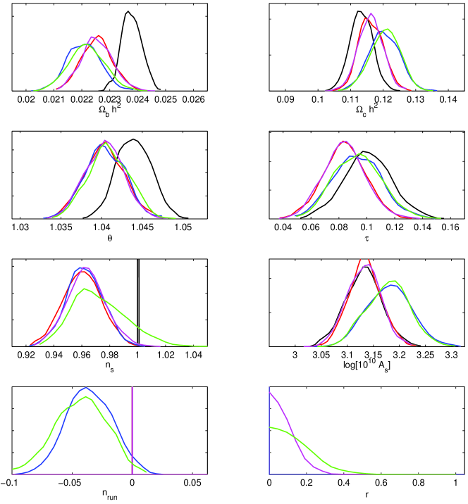
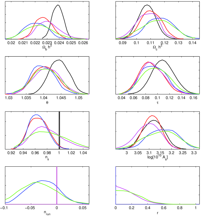
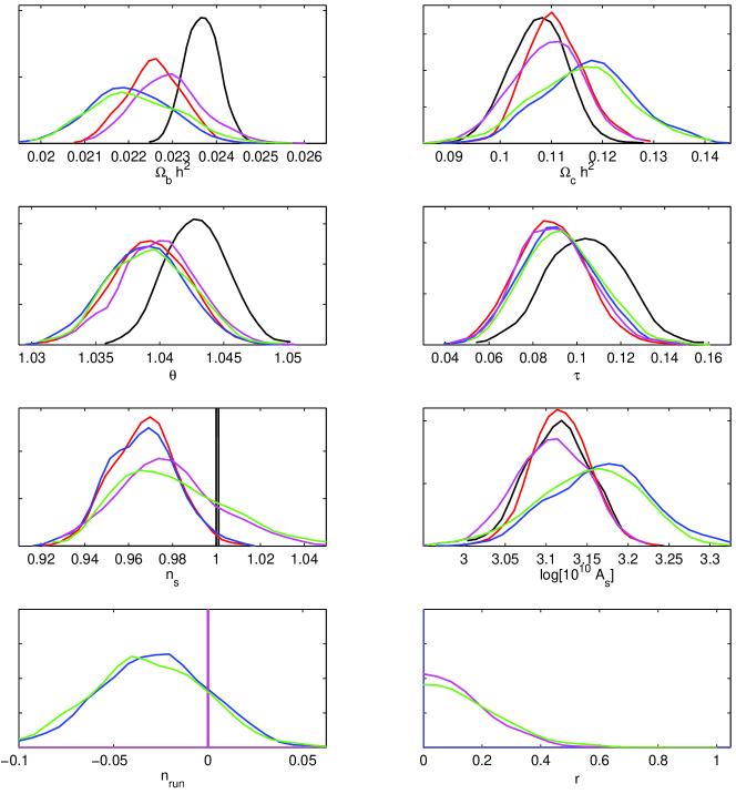
The one-dimensional marginalized posteriors for each parameter, model and data compilation are shown in Figs. 1 (for WMAP 5yr), 2 (for WMAP 7yr), and 3 (for WMAP 7yr+ext). The posteriors are normalized in the usual way, such that the area under each curve is unity. For models where a parameter is not varied (such as the spectral index in the HZ model), a delta function at the appropriate parameter value is the relevant posterior.

In terms of plotting constraints on the power spectrum parameters, the choice of pivot scale $k_{*}$ is important. If it is not optimized, marginalized constraints can appear much weaker than they actually are. We chose the scale that decorrelates the uncertainty on the tilt and the running (in the running model), following the method described in Ref. Cortes:2007ak . This scale is found to be 0.013 Mpc^-1 for the WMAP 5yr and 7yr data and 0.015 Mpc^-1 for the WMAP+ext dataset.

For the Bayesian model averaging, we assume that the prior model probabilities are equal. Variation of this assumption could readily be explored using the quoted evidence values; for instance one might want to downweight HZ as it is not based on a physical model, or models with running as inflationary models with large running are hard to construct. Model averages are carried out by combining the posterior samples from different models weighted by the appropriate model probability.

We do not show a model-averaged result for $A_{\rm s}$, as we did not optimize the pivot scale for the amplitude; in the figures one sees that the central amplitude is shifted in the running models. This means that the amplitude is best determined at some other scale, and a model averaging should only be carried out at that pivot scale if constraining power is not to be lost. In any case one can see by eye that model averaging will have little effect on the constraints on $A_{\rm s}$, which is well determined in all models.

Figure 4: The model-averaged posterior distributions for the spectral index $n_{\rm s}$, using the WMAP 5yr data only (top), the WMAP 7yr data only (middle) and the WMAP 7yr+ext compilation (bottom). The probability distribution includes a delta function around $n_{\rm s}=1$, artificially broadened in the plot by the binning process.

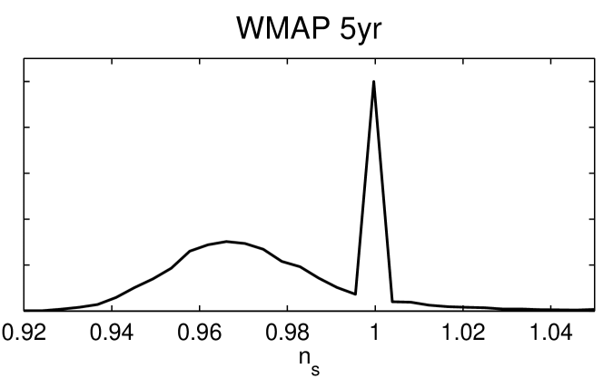
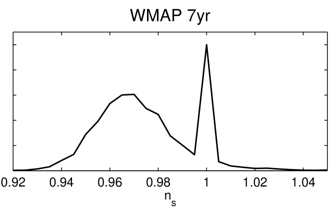
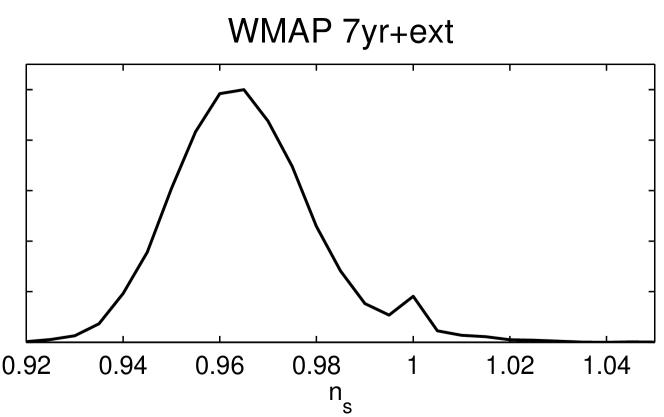
The tilt $n_{\rm s}$ is more interesting, as it is not so well determined due the residual probability that HZ is correct. Its model-averaged posterior is shown in Fig. 4. Note that in analyses with WMAP data alone the HZ ‘spike’ is prominent in the model-averaged posteriors, containing a significant fraction of the posterior probability. Only once other data are brought in does its effect become small. From the complete data compilation, we find that the model-averaged limits on the tilt at the pivot scale are $0.940<n_{\rm s}<1.000$ (95% credible interval), the upper limit being precisely at one as it happens to fall within the delta-function component from the HZ model.

Variation of prior assumptions can modify these results somewhat. Changes to the prior ranges of parameters common to all models, such as $h$ and $\tau$, will have no effect, at least as long as the data constrains the values to lie well within the prior as it does in these cases. Modifying the priors on the parameters that are varied only in some models can shift the results. As an example, we consider doubling the prior range of $n_{\rm s}$, to $[0.6,1.4]$. As the added range fits the data poorly, it has negligible likelihood and this halves the evidence of models in which $n_{\rm s}$ varies, i.e. their log evidences in Table 2 are reduced by $\ln 2\sim 0.69$, which changes the quantitative outcome but not the qualitative one. If one recomputes the 95% confidence range of $n_{\rm s}$ under this assumption the range is unchanged. Changes to the assumed prior model probabilities can be handled similarly.

Figure 5: The model-averaged cumulative probability distribution for the tensor-to-scalar ratio $r$ using the WMAP 7yr+ext compilation. The solid curve gives the probability averaged over all five models, whereas the dashed curve gives the probability averaged just over those models where $r$ is varied (tensor and tensor+running). The dotted line shows the 95% credible limit.

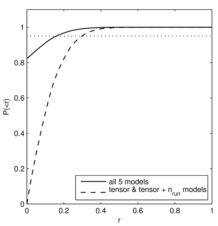
Finally, we consider the tensors. As they are not detected, model uncertainty can have a significant impact by lending support to models in which they are entirely absent, i.e. $r$ is precisely zero. If we average over all five models, the model-averaged 95% upper limit on the tensor-to-scalar ratio is $r<0.16$ (again at the pivot scale). This is indeed somewhat tighter than results from individual models (e.g. the equivalent upper limit from the ‘inflation’ model is $0.18$) because it allows for the possibility of no tensors. Nevertheless, this result is clearly highly prior dependent, and would for instance change if one decided that a logarithmic prior on $r$ were more appropriate.

An alternative tensor limit can be obtained by averaging only over the two models which permit tensors, which gives $r<0.30$. The cumulative model-averaged probabilities for $r$ under both assumptions are shown in Fig. 5. It is clear that any upper limit quoted on the tensor fraction has significant model and prior uncertainty, as well as observational uncertainty.

IV Conclusions

We have illustrated the methodology of Bayesian model averaging using primordial power spectrum estimation. From a Bayesian viewpoint, the purpose of all data analysis is to start with prior information, perhaps entirely theoretically motivated, and take data of increasing quality until the data likelihood is able to convincingly overcome the prior uncertainty. Bayesian model averaging allows us to include the prior model uncertainty as well as the prior parameter uncertainty in this process, and hence offers a more complete incorporation of theoretical uncertainties.

Presently data are unable to decisively distinguish amongst different models for the primordial perturbations, with all five that we discuss remaining viable at some level. Despite that, parameters such as the spectral amplitude that are very accurately measured are quite unaffected by model uncertainty. Parameters moderately well determined, such as $n_{\rm s}$, can see significant effects from model uncertainty, while undetermined parameters such as $r$ are naturally the most sensitive to the increased incorporation of uncertainties.

Bayesian Model Averaging can be used beyond cosmological models to any problem in cosmology or astrophysics where the underlying model is uncertain. This may be uncertainty as to the nature of the physical object (e.g. unresolved galaxies of different species contributing to a background) or with regards to the data analysis (e.g. supernova light curve analysis, where a number of different light curve fitters are available).

As with any Bayesian analysis, the results will have some dependence on the choices of priors, including the model prior probabilities. We should not be afraid of this; the opportunity to choose appropriate priors is our chance to deploy our physical intuition. Readers who prefer different priors are welcome to recalculate if they wish; this is particularly easy for model priors as the evidence ratios we quoted are all that is needed. We also briefly discussed a modification of parameter priors; a full analysis should explore the reasonable range of prior possibilities. Only by combining the full range of prior uncertainties, at both parameter and model level, with observational uncertainties can one obtain the full picture of current understanding.