Fast Overlapping Group Lasso

Abstract

The group Lasso is an extension of the Lasso for feature selection on (predefined) non-overlapping groups of features. The non-overlapping group structure limits its applicability in practice. There have been several recent attempts to study a more general formulation, where groups of features are given, potentially with overlaps between the groups. The resulting optimization is, however, much more challenging to solve due to the group overlaps. In this paper, we consider the efficient optimization of the overlapping group Lasso penalized problem. We reveal several key properties of the proximal operator associated with the overlapping group Lasso, and compute the proximal operator by solving the smooth and convex dual problem, which allows the use of the gradient descent type of algorithms for the optimization. We have performed empirical evaluations using the breast cancer gene expression data set, which consists of 8,141 genes organized into (overlapping) gene sets. Experimental results demonstrate the efficiency and effectiveness of the proposed algorithm.

1 Introduction

Problems with high dimensionality have become common over the recent years. The high dimensionality poses significant challenges in building interpretable models with high prediction accuracy. Regularization has been commonly employed to obtain more stable and interpretable models. A well-known example is the penalization of the $\ell_{1}$ norm of the estimator, known as Lasso [22]. The $\ell_{1}$ norm regularization has achieved great success in many applications. However, in some applications [27], we are interested in finding important explanatory factors in predicting the response variable, where each explanatory factor is represented by a group of input features. In such cases, the selection of important features corresponds to the selection of groups of features. As an extension of Lasso, group Lasso [27] based on the combination of the $\ell_{1}$ norm and the $\ell_{2}$ norm has been proposed for group feature selection, and quite a few efficient algorithms [12, 13, 16] have been proposed for efficient optimization. However, the non-overlapping group structure in group Lasso limits its applicability in practice. For example, in microarray gene expression data analysis, genes may form overlapping groups as each gene may participate in multiple pathways [8].

Several recent work [2, 8, 11, 28] studies the overlapping group Lasso, where groups of features are given, potentially with overlaps between the groups. The resulting optimization is, however, much more challenging to solve due to the group overlaps. When optimizing the overlapping group Lasso problem, one can reformulate it as a second order cone program and solve it by the generic toolboxes, which, however, does not scale well. In [9], an alternating algorithm called SLasso is proposed for solving the equivalent reformulation. However, SLasso involves an expensive matrix inversion at each alternating iteration, and there is no known global convergence rate for such an alternating procedure. It was recently shown in [10] that, for the tree structured group Lasso, the associated proximal operator (or equivalently, the Moreau-Yosida reguralization) [17, 26] can be computed by applying block coordinate ascent in the dual and the algorithm converges in one pass. It was shown independently in [14] that the proximal operator associated with the tree structured group Lasso has a nice analytical solution. However, to the best of our knowledge, there is no analytical solution to the proximal operator associated with the general overlapping group Lasso.

In this paper, we develop an efficient algorithm for the overlapping group Lasso penalized problem via the accelerated gradient descent method. The accelerated gradient descent method has recently received increasing attention in machine learning due to the fast convergence rate even for nonsmooth convex problems. One of the key operations is the computation of the proximal operator associated with the penalty. We reveal several key properties of the proximal operator associated with the overlapping group Lasso penalty, and compute the proximal operator by solving the dual problem. The main contributions of this paper include: (1) we develop a procedure to identify many zero groups in the proximal operator, which dramatically reduces the size of the dual problem to be solved; (2) we show that the dual problem is smooth and convex with Lipschitz continuous gradient, thus can be solved by existing smooth convex optimization tools; and (3) we derive the duality gap between the primal and dual problems, which can be used to check the quality of the solution and determine the convergence of the algorithm. We have performed empirical evaluations using the breast cancer gene expression data set, which consists of 8,141 genes organized into (overlapping) gene sets. Experimental results demonstrate the efficiency and effectiveness of the proposed algorithm.

Notations: $\|\cdot\|$ denotes the Euclidean norm, and $\mathbf{0}$ denotes a vector of zeros. ${\rm SGN}(\cdot)$ and ${\rm sgn}(\cdot)$ are defined in a componentwise fashion as: 1) if $t=0$, then ${\rm SGN}(t)=[-1,1]$ and ${\rm sgn}(t)=0$; 2) if $t>0$, then ${\rm SGN}(t)=\{1\}$ and ${\rm sgn}(t)=1$; and 3) if $t<0$, ${\rm SGN}(t)=\{-1\}$ and ${\rm sgn}(t)=-1$. $G_{i}\subseteq\{1,2,\ldots,p\}$ denotes an index set, and $\mathbf{x}_{G_{i}}$ denote a subvector of $\mathbf{x}$ consisting of the entries indexed by $G_{i}$.

2 The Overlapping Group Lasso

We consider the following overlapping group Lasso penalized problem:

$$\min_{\mathbf{x}\in\mathbb{R}^{p}}f(\mathbf{x})=l(\mathbf{x})+\phi_{\lambda_{2}}^{\lambda_{1}}(\mathbf{x})$$ (1)

where $l(\cdot)$ is a smooth convex loss function, e.g., the least squares loss,

$$\phi_{\lambda_{2}}^{\lambda_{1}}(\mathbf{x})=\lambda_{1}\|\mathbf{x}\|_{1}+\lambda_{2}\sum_{i=1}^{g}w_{i}\|\mathbf{x}_{G_{i}}\|$$ (2)

is the overlapping group Lasso penalty, $\lambda_{1}\geq 0$ and $\lambda_{2}\geq 0$ are regularization parameters, $w_{i}>0,i=1,2,\ldots,g$, $G_{i}\subseteq\{1,2,\ldots,p\}$ contains the indices corresponding to the $i$-th group of features, and $\|\cdot\|$ denotes the Euclidean norm. The $g$ groups of features are pre-specified, and they may overlap. The penalty in (2) is a special case of the more general Composite Absolute Penalty (CAP) family [28]. When the groups are disjoint with $\lambda_{1}=0$ and $\lambda_{2}>0$, the model in (1) reduces to the group Lasso [27]. If $\lambda_{1}>0$ and $\lambda_{2}=0$, then the model in (1) reduces to the standard Lasso [22].

In this paper, we propose to make use of the accelerated gradient descent (AGD) [1, 18, 19] for solving (1), due to its fast convergence rate. The algorithm is called “FoGLasso”, which stands for Fast overlapping Group Lasso. One of the key steps in the proposed FoGLasso algorithm is the computation of the proximal operator associated with the penalty in (2); and we present an efficient algorithm for the computation in the next section.

In FoGLasso, we first construct a model for approximating $f(\cdot)$ at the point $\mathbf{x}$ as:

$$f_{L,\mathbf{x}}(\mathbf{y})=[l(\mathbf{x})+\langle l^{\prime}(\mathbf{x}),\mathbf{y}-\mathbf{x}\rangle]+\phi_{\lambda_{1}}^{\lambda_{2}}(\mathbf{y})+\frac{L}{2}\|\mathbf{y}-\mathbf{x}\|^{2},$$ (3)

where $L>0$. The model $f_{L,\mathbf{x}}(\mathbf{y})$ consists of the first-order Taylor expansion of the smooth function $l(\cdot)$ at the point $\mathbf{x}$, the non-smooth penalty $\phi_{\lambda_{1}}^{\lambda_{2}}(\mathbf{x})$, and a regularization term $\frac{L}{2}\|\mathbf{y}-\mathbf{x}\|^{2}$. Next, a sequence of approximate solutions $\{\mathbf{x}_{i}\}$ is computed as follows:

$$\mathbf{x}_{i+1}=\arg\min_{\mathbf{y}}f_{L_{i},\mathbf{s}_{i}}(\mathbf{y})$$ (4)

where the search point $\mathbf{s}_{i}$ is an affine combination of $\mathbf{x}_{i-1}$ and $\mathbf{x}_{i}$ as

$$\mathbf{s}_{i}=\mathbf{x}_{i}+\beta_{i}(\mathbf{x}_{i}-\mathbf{x}_{i-1}),$$ (5)

for a properly chosen coefficient $\beta_{i}$, $L_{i}$ is determined by the line search according to the Armijo-Goldstein rule so that $L_{i}$ should be appropriate for $\mathbf{s}_{i}$, i.e., $f(\mathbf{x}_{i+1})\leq f_{L,\mathbf{s}_{i}}(\mathbf{x}_{i+1})$. Following the analysis in [1, 19], we can show that FoGLasso achieves a convergence rate of $O(1/k^{2})$ for $k$ iterations, which is optimal among first-order methods. A key building block in FoGLasso is the minimization of (3), whose solution is known as the proximal operator [7, 17]. The computation of the proximal operator is the main technical contribution of this paper. The pseudo-code of FoGLasso is summarized in Algorithm 1, where the proximal operator $\pi(\cdot)$ is defined in (6). In practice, we can terminate Algorithm 1 if the change of the function values corresponding to adjacent iterations is within a small value, say $10^{-5}$.

Algorithm 1 The FoGLasso Algorithm

0:  $L_{0}>0,\mathbf{x}_{0},k$

0:  $\mathbf{x}_{k+1}$

1:  Initialize $\mathbf{x}_{1}=\mathbf{x}_{0}$, $\alpha_{-1}=0$, $\alpha_{0}=1$, and $L=L_{0}$.

2:  for $i=1$ to $k$ do

3:     Set $\beta_{i}=\frac{\alpha_{i-2}-1}{\alpha_{i-1}}$, $\mathbf{s}_{i}=\mathbf{x}_{i}+\beta_{i}(\mathbf{x}_{i}-\mathbf{x}_{i-1})$

4:     Find the smallest $L=2^{j}L_{i-1},j=0,1,\ldots$ such that $f(\mathbf{x}_{i+1})\leq f_{L,\mathbf{s}_{i}}(\mathbf{x}_{i+1})$ holds, where $\mathbf{x}_{i+1}=\pi_{\lambda_{2}/L}^{\lambda_{1}/L}(\mathbf{s}_{i}-\frac{1}{L}l^{\prime}(\mathbf{s}_{i}))$

5:     Set $L_{i}=L$ and $\alpha_{i+1}=\frac{1+\sqrt{1+4\alpha_{i}^{2}}}{2}$

6:  end for

3 The Associated Proximal Operator and Its Efficient Computation

The proximal operator associated with the overlapping group Lasso penalty is defined as follows:

$$\pi_{\lambda_{2}}^{\lambda_{1}}(\mathbf{v})=\arg\min_{\mathbf{x}\in\mathbb{R}^{p}}\left\{g_{\lambda_{2}}^{\lambda_{1}}(\mathbf{x})\equiv\frac{1}{2}\|\mathbf{x}-\mathbf{v}\|^{2}+\lambda_{1}\|\mathbf{x}\|_{1}+\lambda_{2}\sum_{i=1}^{g}w_{i}\|\mathbf{x}_{G_{i}}\|\right\},$$ (6)

which is a special case of (1) by setting $l(\mathbf{x})=\frac{1}{2}\|\mathbf{x}-\mathbf{v}\|^{2}$. It can be verified that the approximate solution $x_{i+1}$ in (4) is given by $\mathbf{x}_{i+1}=\pi_{\lambda_{2}/L_{i}}^{\lambda_{1}/L_{i}}(\mathbf{s}_{i}-\frac{1}{L_{i}}l^{\prime}(\mathbf{s}_{i}))$. Recently, it has been shown in [10, 14, 15] that, the efficient computation of the proximal operator is key to many sparse learning algorithms [15, Section 2]. Next, we focus on the efficient computation of $\pi_{\lambda_{2}}^{\lambda_{1}}(\mathbf{v})$ in (6) for a given $\mathbf{v}$.

3.1 Key Properties of the Proximal Operator

We first reveal several basic properties of the proximal operator $\pi_{\lambda_{2}}^{\lambda_{1}}(\mathbf{v})$.

Lemma 1.

Suppose that $\lambda_{1},\lambda_{2}\geq 0$, and $w_{i}>0$, for $i=1,2,\ldots,g$. Let $\mathbf{x}^{*}=\pi_{\lambda_{2}}^{\lambda_{1}}(\mathbf{v})$. The following holds: 1) if $v_{i}>0$, then $0\leq x_{i}^{*}\leq v_{i}$; 2) if $v_{i}<0$, then $v_{i}\leq x_{i}^{*}\leq 0$; 3) if $v_{i}=0$, then $x_{i}^{*}=0$; 4) ${\rm SGN}(\mathbf{v})\subseteq{\rm SGN}(\mathbf{x}^{*})$; and 5) $\pi_{\lambda_{2}}^{\lambda_{1}}(\mathbf{v})={\rm sgn}(\mathbf{v})\odot\pi_{\lambda_{2}}^{\lambda_{1}}(|\mathbf{v}|)$.

Proof.

When $\lambda_{1},\lambda_{2}\geq 0$, and $w_{i}\geq 0$, for $i=1,2,\ldots,g$, the objective function $g_{\lambda_{2}}^{\lambda_{1}}(\cdot)$ is strictly convex, thus $\mathbf{x}^{*}$ is the unique minimizer. We first show if $v_{i}>0$, then $0\leq x_{i}^{*}\leq v_{i}$. If $x_{i}^{*}>v_{i}$, then we can construct a $\mathbf{\hat{x}}$ as follows: $\hat{x}_{j}=x_{j}^{*},j\neq i$ and $\hat{x}_{i}=v_{i}$. Similarly, if $x_{i}^{*}<0$, then we can construct a $\mathbf{\hat{x}}$ as follows: $\hat{x}_{j}=x_{j}^{*},j\neq i$ and $\hat{x}_{i}=0$. It is easy to verify that $\mathbf{\hat{x}}$ achieves a lower objective function value than $\mathbf{x}^{*}$ in both cases. We can prove the second and the third properties using similar arguments. Finally, we can prove the fourth and the fifth properties using the definition of $\mbox{SGN}(\cdot)$ and the first three properties. ∎

Next, we show that $\pi_{\lambda_{2}}^{\lambda_{1}}(\cdot)$ can be directly derived from $\pi_{\lambda_{2}}^{0}(\cdot)$ by soft-thresholding. Thus, we only need to focus on the simple case when $\lambda_{1}=0$. This simplifies the optimization in (6).

Theorem 1.

Let

$$\mathbf{u}={\rm sgn}(\mathbf{v})\odot\max(|\mathbf{v}|-\lambda_{1},0),$$ (7)

$$\pi_{\lambda_{2}}^{0}(\mathbf{u})=\arg\min_{\mathbf{x}\in\mathbb{R}^{p}}\left\{h_{\lambda_{2}}(\mathbf{x})\equiv\frac{1}{2}\|\mathbf{x}-\mathbf{u}\|^{2}+\lambda_{2}\sum_{i=1}^{g}w_{i}\|\mathbf{x}_{G_{i}}\|\right\}.$$ (8)

The following holds:

$$\pi_{\lambda_{2}}^{\lambda_{1}}(\mathbf{v})=\pi_{\lambda_{2}}^{0}(\mathbf{u}).$$ (9)

Proof.

Denote the unique minimizer of $h_{\lambda_{2}}(\cdot)$ as $\mathbf{x}^{*}$. The sufficient and necessary condition for the optimality of $\mathbf{x}^{*}$ is:

$$\mathbf{0}\in\partial h_{\lambda_{2}}(\mathbf{x}^{*})=\mathbf{x}^{*}-\mathbf{u}+\partial\phi_{\lambda_{2}}^{0}(\mathbf{x}^{*}),$$ (10)

where $\partial h_{\lambda_{2}}(\mathbf{x})$ and $\partial\phi_{\lambda_{2}}^{0}(\mathbf{x})$ are the subdifferential sets of $h_{\lambda_{2}}(\cdot)$ and $\phi_{\lambda_{2}}^{0}(\cdot)$ at $\mathbf{x}$, respectively.

To prove (9), it suffices to show $\mathbf{0}\in\partial g_{\lambda_{2}}^{\lambda_{1}}(\mathbf{x}^{*})$. The subdifferential of $g_{\lambda_{2}}^{\lambda_{1}}(\cdot)$ at $\mathbf{x}^{*}$ is given by

$$\partial g_{\lambda_{2}}^{\lambda_{1}}(\mathbf{x}^{*})=\mathbf{x}^{*}-\mathbf{v}+\partial\phi_{\lambda_{2}}^{\lambda_{1}}(\mathbf{x}^{*})=\mathbf{x}^{*}-\mathbf{v}+\lambda_{1}{\rm SGN}(\mathbf{x}^{*})+\partial\phi_{\lambda_{2}}^{0}(\mathbf{x}^{*}).$$ (11)

It follows from (7) that $\mathbf{u}\in\mathbf{v}-\lambda_{1}\mbox{SGN}(\mathbf{u})$. Using the fourth property in Lemma 1, we have $\mbox{SGN}(\mathbf{u})\subseteq{\rm SGN}(\mathbf{x}^{*})$. Thus,

$$\mathbf{u}\in\mathbf{v}-\lambda_{1}{\rm SGN}(\mathbf{x}^{*}).$$ (12)

It follows from (10)-(12) that $\mathbf{0}\in\partial g_{\lambda_{2}}^{\lambda_{1}}(\mathbf{x}^{*})$. ∎

It follows from Theorem 1 that, we only need to focus on the optimization of (8) in the following discussion. The difficulty in the optimization of (8) lies in the large number of groups that may overlap. In practice, many groups will be zero, thus achieving a sparse solution. However, the zero groups are not known in advance. The key question we aim to address is how we can identify as many zero groups as possible to reduce the complexity of the optimization. We present in the next lemma a sufficient condition for a group to be zero.

Lemma 2.

Denote the minimizer of $h_{\lambda_{2}}(\cdot)$ in (8) by $\mathbf{x}^{*}$. If the $i$-th group satisfies $\|\mathbf{u}_{G_{i}}\|\leq\lambda_{2}w_{i}$, then $\mathbf{x}_{G_{i}}^{*}=\mathbf{0}$, i.e., the $i$-th group is zero.

Proof.

We decompose $h_{\lambda_{2}}(\mathbf{x})$ into two parts as follows:

$$h_{\lambda_{2}}(\mathbf{x})=\left\{\frac{1}{2}\|\mathbf{x}_{G_{i}}-\mathbf{u}_{G_{i}}\|^{2}+\lambda_{2}w_{i}\|\mathbf{x}_{G_{i}}\|\right\}+\left\{\frac{1}{2}\|\mathbf{x}_{\overline{G}_{i}}-\mathbf{u}_{\overline{G}_{i}}\|^{2}+\lambda_{2}\sum_{j\neq i}w_{j}\|\mathbf{x}_{G_{j}}\|\right\},$$ (13)

where $\overline{G}_{i}=\{1,2,\ldots,p\}-G_{i}$ is the complementary set of $G_{i}$. We consider the minimization of $h_{\lambda_{2}}(\mathbf{x})$ in terms of $\mathbf{x}_{G_{i}}$ when $\mathbf{x}_{\overline{G}_{i}}=\mathbf{x}^{*}_{\overline{G}_{i}}$ is fixed. It can be verified that if $\|\mathbf{u}_{G_{i}}\|\leq\lambda_{2}w_{i}$, then $\mathbf{x}_{G_{i}}^{*}=\mathbf{0}$ minimizes both terms in (13) simultaneously. Thus we have $\mathbf{x}_{G_{i}}^{*}=\mathbf{0}$. ∎

Lemma 2 may not identify many true zero groups due to the strong condition imposed. The lemma below weakens the condition in Lemma 2. Intuitively, for a group $G_{i}$, we first identify all existing zero groups that overlap with $G_{i}$, and then compute the overlapping index subset $S_{i}$ of $G_{i}$ as:

$$S_{i}=\bigcup_{j\neq i,\mathbf{x}^{*}_{G_{j}}=\mathbf{0}}(G_{j}\cap G_{i}).$$ (14)

We can show that $\mathbf{x}^{*}_{G_{i}}=\mathbf{0}$ if $\|\mathbf{u}_{G_{i}-S_{i}}\|\leq\lambda_{2}w_{i}$ is satisfied. Note that this condition is much weaker than the condition in Lemma 2, which requires that $\|\mathbf{u}_{G_{i}}\|\leq\lambda_{2}w_{i}$.

Lemma 3.

Denote the minimizer of $h_{\lambda_{2}}(\cdot)$ by $\mathbf{x}^{*}$. Let $S_{i}$, a subset of $G_{i}$, be defined in (14). If $\|\mathbf{u}_{G_{i}-S_{i}}\|\leq\lambda_{2}w_{i}$ holds, then $\mathbf{x}^{*}_{G_{i}}=\mathbf{0}$.

The proof of Lemma 3 follows similar arguments in Lemma 2 and is omitted. Lemma 3 naturally leads to an iterative procedure for identifying the zero groups: For each group $G_{i}$, if $\|\mathbf{u}_{G_{i}}\|\leq\lambda_{2}w_{i}$, then we set $\mathbf{u}_{G_{i}}=\mathbf{0}$; we cycle through all groups repeatedly until $\mathbf{u}$ does not change.

Let $p^{\prime}=|\{u_{i}:u_{i}\neq 0\}|$ be the number of nonzero elements in $\mathbf{u}$, $g^{\prime}=|\{\mathbf{u}_{G_{i}}:\mathbf{u}_{G_{i}}\neq\mathbf{0}\}|$ be the number of the nonzero groups, and $\mathbf{x}^{*}$ denote the minimizer of $h_{\lambda_{2}}(\cdot)$. It follows from Lemma 3 and Lemma 1 that, if $u_{i}=0$, then $x^{*}_{i}=0$. Therefore, by applying the above iterative procedure, we can find the minimizer of (8) by solving a reduced problem that has $p^{\prime}\leq p$ variables and $g^{\prime}\leq g$ groups. With some abuse of notation, we still use (8) to denote the resulting reduced problem. In addition, from Lemma 1, we only focus on $\mathbf{u}>0$ in the following discussion, and the analysis can be easily generalized to the general $\mathbf{u}$.

3.2 Reformulation as an Equivalent Smooth Convex Optimization Problem

It follows from the first property of Lemma 1 that, we can rewrite (8) as:

$$\pi_{\lambda_{2}}^{0}(\mathbf{u})=\arg\min_{\mathbf{x}\in\mathbb{R}^{p}:\mathbf{x}\geq\mathbf{0}}\left\{h_{\lambda_{2}}(\mathbf{x})\equiv\frac{1}{2}\|\mathbf{x}-\mathbf{u}\|^{2}+\lambda_{2}\sum_{i=1}^{g}w_{i}\|\mathbf{x}_{G_{i}}\|\right\},$$ (15)

where the minimizer of $h_{\lambda_{2}}(\cdot)$ is constrained to be non-negative due to $\mathbf{u}>0$.

Making use of the dual norm of the Euclidean norm $\|\cdot\|$, we can rewrite $h_{\lambda_{2}}(\mathbf{x})$ as:

$$h_{\lambda_{2}}(\mathbf{x})=\max_{Y\in\Omega}\frac{1}{2}\|\mathbf{x}-\mathbf{u}\|^{2}+\sum_{i=1}^{g}\langle\mathbf{x},Y^{i}\rangle,$$ (16)

where $\Omega$ is defined as follows:

$$\Omega=\{Y\in\mathbb{R}^{p\times g}:Y^{i}_{\overline{G}_{i}}=\mathbf{0},\|Y^{i}\|\leq\lambda_{2}w_{i},i=1,2,\ldots,g\},$$

$\overline{G}_{i}$ is the complementary set of $G_{i}$, $Y$ is a sparse matrix satisfying $Y_{ij}=0$ if the $i$-th feature does not belong to the $j$-th group, i.e., $i\not\in G_{j}$, and $Y^{i}$ denotes the $i$-th column of $Y$. As a result, we can reformulate (15) as the following min-max problem:

$$\min_{\mathbf{x}\in\mathbb{R}^{p}:\mathbf{x}\geq\mathbf{0}}\mbox{ }\max_{Y\in\Omega}\left\{\psi(\mathbf{x},Y)=\frac{1}{2}\|\mathbf{x}-\mathbf{u}\|^{2}+\langle\mathbf{x},Y\mathbf{e}\rangle\right\},$$ (17)

where $\mathbf{e}\in\mathbb{R}^{g}$ is a vector of ones. It is easy to verify that $\psi(\mathbf{x},Y)$ is convex in $\mathbf{x}$ and concave in $Y$, and the constraint sets are closed convex for both $\mathbf{x}$ and $Y$. Thus, (17) has a saddle point, and the min-max can be exchanged.

It is easy to verify that for a given $Y$, the optimal $\mathbf{x}$ minimizing $\psi(\mathbf{x},Y)$ in (17) is given by

$$\mathbf{x}=\max(\mathbf{u}-Y\mathbf{e},\mathbf{0}).$$ (18)

Plugging (18) into (17), we obtain the following minimization problem with regard to $Y$:

$$\min_{Y\in\mathbb{R}^{p\times g}:Y\in\Omega}\left\{\omega(Y)=-\psi(\max(\mathbf{u}-Y\mathbf{e},\mathbf{0}),Y)\right\}.$$ (19)

Our methodology for minimizing $h_{\lambda_{2}}(\cdot)$ defined in (8) is to first solve (19), and then construct the solution to $h_{\lambda_{2}}(\cdot)$ via (18). We show in Theorem 2 below that the function $\omega(\cdot)$ is continuously differentiable with Lipschitz continuous gradient. Therefore, we convert the non-smooth problem (15) to the smooth problem (19), making the smooth convex optimization tools applicable.

Theorem 2.

The function $\omega(Y)$ is convex and continuously differentiable with

$$\omega^{\prime}(Y)=-\max(\mathbf{u}-Y\mathbf{e},\mathbf{0})\mathbf{e}^{\rm T}.$$ (20)

In addition, $\omega^{\prime}(Y)$ is Lipschitz continuous with constant $g^{2}$, i.e.,

$$\|\omega^{\prime}(Y_{1})-\omega^{\prime}(Y_{2})\|_{F}\leq g^{2}\|Y_{1}-Y_{2}\|_{F},\,\,\,\,\forall\,\,Y_{1},Y_{2}\in\mathbb{R}^{p\times g}.$$ (21)

To prove Theorem 2, we first present two technical lemmas. The first lemma is related to the optimal value function [3, 5], and it was used in a recent study [25] on infinite kernel learning.

Lemma 4.

[3, Theorem 4.1] Let $X$ be a metric space and $U$ be a normed space. Suppose that for all $\mathbf{x}\in X$, the function $\psi(\mathbf{x},\cdot)$ is differentiable and that $\psi(\mathbf{x},Y)$ and $D_{Y}\psi(\mathbf{x},Y)$ (the partial derivative of $\psi(\mathbf{x},Y)$ with respect to $Y$) are continuous on $X\times U$. Let $\Phi$ be a compact subset of $X$. Define the optimal value function as $\varphi(Y)=\inf_{\mathbf{x}\in\Phi}\psi(\mathbf{x},Y)$. The optimal value function $\varphi(Y)$ is directionally differentiable. In addition, if $\forall Y\in U$, $\psi(\cdot,Y)$ has a unique minimizer $\mathbf{x}(Y)$ over $\Phi$, then $\varphi(Y)$ is differentiable at $Y$ and the gradient of $\varphi(Y)$ is given by $\varphi^{\prime}(Y)=D_{Y}\psi(\mathbf{x}(Y),Y)$.

The second lemma shows that the operator $\mathbf{y}=\max(\mathbf{x},\mathbf{0})$ is non-expansive.

Lemma 5.

$\forall\mathbf{x},\mathbf{y}\in\mathbb{R}^{p}$, we have $\|\max(\mathbf{x},\mathbf{0})-\max(\mathbf{y},\mathbf{0})\|\leq\|\mathbf{x}-\mathbf{y}\|$.

Proof.

The results follows since $|\max(x,0)-\max(y,0)|\leq|x-y|$, $\forall x,y\in\mathbb{R}$. ∎

Proof of Theorem 2: To prove the differentiability of $\omega(Y)$, we apply Lemma 4 with $X=\mathbb{R}^{p}$, $U=\mathbb{R}^{p\times g}$ and $\Phi=\{\mathbf{x}\in X:\mathbf{u}+\lambda_{2}\sum w_{i}\mathbf{e}\geq\mathbf{x}\geq\mathbf{0}\}$. It is easy to verify that 1) $\psi(\mathbf{x},\cdot)$ is differentiable; 2) $\psi(\mathbf{x},Y)$ and $D_{Y}\psi(\mathbf{x},Y)=\mathbf{x}\mathbf{e}^{\rm T}$ are continuous on $X\times U$; 3) $\Phi$ be a compact subset of $X$; and 4) $\forall Y\in U$, $\psi(\mathbf{x},Y)$ has a unique minimizer $\mathbf{x}(Y)=\max(\mathbf{u}-Y\mathbf{e},\mathbf{0})$ over $\Phi$. Note that, the last result follows from $\mathbf{u}>0$ and $\mathbf{u}-Y\mathbf{e}\leq\mathbf{u}+\lambda_{2}\sum w_{i}\mathbf{e}$, where the latter inequality utilizes $\|Y^{i}\|\leq\lambda_{2}w_{i}$; and this indicates that $\mathbf{x}(Y)=\max(\mathbf{u}-Y\mathbf{e},\mathbf{0})=\arg\min_{\mathbf{x}}\psi(\mathbf{x},Y)=\arg\min_{\mathbf{x}\in\Phi}\psi(\mathbf{x},Y)$. It follows from Lemma 4 that

$$\varphi(Y)=\inf_{\mathbf{x}\in\Phi}\psi(\mathbf{x},Y)=\psi(\max(\mathbf{u}-Y\mathbf{e},\mathbf{0}),Y)$$

is differentiable with $\varphi^{\prime}(Y)=\max(\mathbf{u}-Y\mathbf{e},\mathbf{0})\mathbf{e}^{\rm T}$.

In (17), $\psi(\mathbf{x},Y)$ is convex in $\mathbf{x}$ and concave in $Y$, and the constraint sets are closed convex for both $\mathbf{x}$ and $Y$, thus the existence of the saddle point is guaranteed by the well-known von Neumann Lemma [18, Chapter 5.1]. As a result,

$$\varphi(Y)=\inf_{\mathbf{x}\in\Phi}\psi(\mathbf{x},Y)=\psi(\max(\mathbf{u}-Y\mathbf{e},\mathbf{0}),Y)$$

is concave, and $\omega(Y)=-\varphi(Y)$ is convex. For any $Y_{1},Y_{2}$, we have

$$\|\omega^{\prime}(Y_{1})-\omega^{\prime}(Y_{2})\|_{F}= \|\max(\mathbf{u}-Y_{1}\mathbf{e},\mathbf{0})\mathbf{e}^{\rm T}-\max(\mathbf{u}-Y_{2}\mathbf{e},\mathbf{0})\mathbf{e}^{\rm T}\|_{F}$$ (22)

$$\leq \|\mathbf{e}\|\times\|\max(\mathbf{u}-Y_{1}\mathbf{e},\mathbf{0})-\max(\mathbf{u}-Y_{2}\mathbf{e},\mathbf{0})\|$$

$$\leq \|\mathbf{e}\|\times\|(Y_{1}-Y_{2})\mathbf{e}\|$$

$$\leq g^{2}\|Y_{1}-Y_{2}\|_{F},$$

where the second inequality follows from Lemma 5. We prove (21). $\Box$

From Theorem 2, the problem in (19) is a constrained smooth convex optimization problem, and existing solvers for constrained smooth convex optimization can be applied. In this paper, we employ the accelerated gradient descent to solve (19), due to its fast convergence property. Note that, the Euclidean projection onto the set $\Omega$ can be computed in the closed form. We would like to emphasize here that, the problem (19) may have a much smaller size than (6).

3.3 Computing the Duality Gap

We show how to estimate the duality gap of the min-max problem (17), which can be used to check the quality of the solution and determine the convergence of the algorithm.

For any given approximate solution $\tilde{Y}\in\Omega$ for $\omega(Y)$, we can construct the approximate solution $\mathbf{\tilde{x}}=\max(\mathbf{u}-\tilde{Y}\mathbf{e},\mathbf{0})$ for $h_{\lambda_{2}}(\mathbf{x})$. The duality gap for the min-max problem (17) at the point $(\mathbf{\tilde{x}},\tilde{Y})$ can be computed as:

$$\mbox{gap}(\tilde{Y})=\max_{Y\in\Omega}\psi(\tilde{\mathbf{x}},Y)-\min_{\mathbf{x}\in\mathbb{R}^{p}:\mathbf{x}\geq\mathbf{0}}\psi(\mathbf{x},\tilde{Y}).$$ (23)

The main result of this subsection is summarized in the following theorem:

Theorem 3.

Let ${\rm gap}(\tilde{Y})$ be the duality gap defined in (23). Then, the following holds:

$${\rm gap}(\tilde{Y})=\lambda_{2}\sum_{i=1}^{g}(w_{i}\|\tilde{\mathbf{x}}_{G_{i}}\|-\langle\tilde{\mathbf{x}}_{G_{i}},\tilde{Y}_{G_{i}}^{i}\rangle).$$ (24)

In addition, we have

$$\omega(\tilde{Y})-\omega(Y^{*})\leq{\rm gap}(\tilde{Y}),$$ (25)

$$h(\tilde{\mathbf{x}})-h(\mathbf{x}^{*})\leq{\rm gap}(\tilde{Y}).$$ (26)

Proof.

Denote $(\mathbf{x}^{*},Y^{*})$ as the optimal solution to the min-max problem (17). From (16)-(19), we have

$$-\omega(\tilde{Y})=\psi(\tilde{\mathbf{x}},\tilde{Y})=\min_{\mathbf{x}\in\mathbb{R}^{p}:\mathbf{x}\geq\mathbf{0}}\psi(\mathbf{x},\tilde{Y})\leq\psi(\mathbf{x}^{*},\tilde{Y}),$$ (27)

$$\psi(\mathbf{x}^{*},\tilde{Y})\leq\max_{Y\in\Omega}\psi(\mathbf{x}^{*},Y)=\psi(\mathbf{x}^{*},Y^{*})=-\omega(Y^{*}),$$ (28)

$$h_{\lambda_{2}}(\mathbf{x}^{*})=\psi(\mathbf{x}^{*},Y^{*})=\min_{\mathbf{x}\in\mathbb{R}^{p}:\mathbf{x}\geq\mathbf{0}}\psi(\mathbf{x},Y^{*})\leq\psi(\tilde{\mathbf{x}},Y^{*}),$$ (29)

$$\psi(\tilde{\mathbf{x}},Y^{*})\leq\max_{Y\in\Omega}\psi(\tilde{\mathbf{x}},Y)=h_{\lambda_{2}}(\tilde{\mathbf{x}}).$$ (30)

Incorporating (15), (27)-(30), we prove (24)-(26). ∎

In our experiments, we terminate the algorithm when the estimated duality gap is less than $10^{-10}$.

4 Experiments

We have conducted experiments to evaluate the efficiency of the proposed algorithm using the breast cancer gene expression data set [23], which consists of 8,141 genes in 295 breast cancer tumors (78 metastatic and 217 non-metastatic). For the sake of analyzing microarrays in terms of biologically meaningful gene sets, different approaches have been used to organize the genes into (overlapping) gene sets. In our experiments, we follow [8] and employ the following two approaches for generating the overlapping gene sets (groups): pathways [21] and edges [4]. For pathways, the canonical pathways from the Molecular Signatures Database (MSigDB) [21] are used. It contains 639 groups of genes, of which 637 groups involve the genes in our study. The statistics of the 637 gene groups are summarized as follows: the average number of genes in each group is 23.7, the largest gene group has 213 genes, and 3,510 genes appear in these 637 groups with an average appearance frequency of about 4. For edges, the network built in [4] will be used, and we follow [8] to extract 42,594 edges from the network, leading to 42,594 overlapping gene sets of size 2. All 8,141 genes appear in the 42,594 groups with an average appearance frequency of about 10.

Figure 1: Comparison of SLasso [9] and our proposed FoGLasso algorithm in terms of computational time (in seconds) when different numbers of genes (variables) are involved. The computation time is reported in the logarithmic scale.

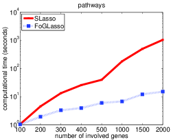
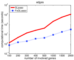
Efficiency of the Proposed FoGLasso We compare our proposed FoGLasso with the SLasso algorithm developed by Jenatton et al. [9] for solving (1) with the least squares loss $l(\mathbf{x})=\frac{1}{2}\|A\mathbf{x}-\mathbf{b}\|^{2}$. The experimental settings are as follows: we set $w_{i}=\sqrt{|G_{i}|}$, and $\lambda_{1}=\lambda_{2}=\rho\times\lambda_{1}^{\max}$, where $|G_{i}|$ denotes the size of the $i$-th group $G_{i}$, $\lambda_{1}^{\max}=\|A^{\rm T}\mathbf{b}\|_{\infty}$ (the zero point is a solution to (1) if $\lambda_{1}\geq\lambda_{1}^{\max}$), and $\rho$ is chosen from the set $\{5\times 10^{-1},2\times 10^{-1},1\times 10^{-1},5\times 10^{-2},2\times 10^{-2},1\times 10^{-2},5\times 10^{-3},2\times 10^{-3},1\times 10^{-3}\}$. For a given $\rho$, we first run SLasso, and then run our proposed FoGLasso until it achieves an objective function value smaller than or equal to that of SLasso. For both SLasso and FoGLasso, we apply the “warm” start technique, i.e., using the solution corresponding to the larger regularization parameter as the “warm” start for the smaller one. We vary the number of genes involved, and report the total computational time (seconds) including all nine regularization parameters in Figure 1 and Table 1. We can observe that, 1) our proposed FoGLasso is much more efficient than SLasso; 2) the advantage of FoGLasso over SLasso in efficiency grows with the increasing number of genes (variables). For example, with the grouping by pathways, FoGLasso is about 25 and 70 times faster than SLasso for 1000 and 2000 genes (variables), respectively; and 3) the efficiency on edges is inferior to that on pathways, due to the larger number of overlapping groups. These results verify the efficiency of the proposed FoGLasso algorithm based on the efficient procedure for computing the proximal operator presented in Section 3.

Table 1: Scalability study of the proposed FoGLasso algorithm under different numbers ($p$) of genes involved. The reported results are the total computational time (seconds) including all nine regularization parameter values.

$p$	3000	4000	5000	6000	7000	8141
pathways	37.6	48.3	62.5	68.7	86.2	99.7
edges	58.8	84.8	102.7	140.8	173.3	247.8

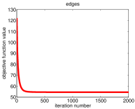
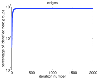
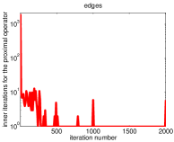
Computation of the Proximal Operator In this experiment, we run FoGLasso on the breast cancer data set using all 8,141 genes. We terminate FoGLasso if the change of the objective function value is less than $10^{-5}$. We use the 42,594 edges to generate the overlapping groups. We obtain similar results for the 637 groups based on pathways. We set $\rho=0.01$. The results are shown in Figure 2. The left plot shows that the objective function value decreases rapidly in the proposed FoGLasso. In the middle plot, we report the percentage of the identified zero groups by applying Lemma 3. Our experimental result shows that, 1) after 16 iterations, 50% of the zero groups are correctly identified; and 2) after 50 iterations, 80% of the zero groups are identified. Therefore, with Lemma 3, we can significantly reduce the problem size of the subsequent dual reformulation (see Section 3.1). In the right plot of Figure 2, we present the number of inner iterations for solving the proximal operator via the dual reformulation. We attribute the decreasing number of inner iterations to 1) the size of the reduced problem is decreasing when many zero groups are identified (see the middle plot); and 2) in solving the dual reformulation, we can apply the $Y$ computed in the previous iteration as the “warm” start for computing the proximal operator in the next iteration.

Figure 2: Performance of the computation of the proximal operator in FoGLasso. The left plot shows the objective function value during the FoGLasso iteration. The middle plot shows the percentage of the identified zero groups by applying Lemma 3. The right plot shows the number of inner iterations for achieving the duality gap less than $10^{-10}$ when one solves the proximal operator via the dual reformulation (see Section 3.2).

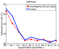
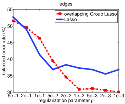
Classification Performance We compare the classification performance of the overlapping group Lasso with Lasso. We use 60% samples for training and the rest 40% for testing. To deal with the imbalance of the positive and negative samples, we make use of the balanced error rate [6], which is defined as the average error of two classes. We report the results averaged over 10 runs in Figure 3. Our results show that: 1) with the overlapping pathways, overlapping Lasso and Lasso achieve comparable classification performance; 2) with the overlapping edges, overlapping Lasso outperforms Lasso; and 3) the performance based on edges is better than that based on the pathways in our experiment.

Figure 3: Comparison of overlapping group Lasso and Lasso in terms of the balanced error rate. The left plot shows the classification performance with overlapping pathways; and the right plot shows the result with the overlapping edges.

5 Conclusion

In this paper, we consider the efficient optimization of the overlapping group Lasso penalized problem based on the accelerated gradient descent method. We reveal several key properties of the proximal operator associated with the overlapping group Lasso, and compute the proximal operator via solving the smooth and convex dual problem. Numerical experiments on the breast cancer data set demonstrate the efficiency of the proposed algorithm. Our experimental results also show the benefit of the overlapping group Lasso in comparison with Lasso. In the future, we plan to apply the proposed algorithm to other real-world applications involving overlapping groups.

References

- [1] A. Beck and M. Teboulle. A fast iterative shrinkage-thresholding algorithm for linear inverse problems. SIAM Journal on Imaging Sciences, 2(1):183–202, 2009.
- [2] H. D. Bondell and B. J. Reich. Simultaneous regression shrinkage, variable selection and clustering of predictors with oscar. Biometrics, 64:115–123, 2008.
- [3] J. F. Bonnans and A. Shapiro. Optimization problems with perturbations: A guided tour. SIAM Review, 40(2):228–264, 1998.
- [4] H. Y. Chuang, E. Lee, Y. T. Liu, D. Lee, and T. Ideker. Network-based classification of breast cancer metastasis. Molecular Systems Biology, 3(140), 2007.
- [5] J. M. Danskin. The theory of max-min and its applications to weapons allocation problems. Springer-Verlag, New York, 1967.
- [6] I. Guyon, A. B. Hur, S. Gunn, and G. Dror. Result analysis of the nips 2003 feature selection challenge. In Neural Information Processing Systems, pages 545–552, 2004.
- [7] J. Hiriart-Urruty and C. Lemaréchal. Convex Analysis and Minimization Algorithms I & II. Springer Verlag, Berlin, 1993.
- [8] L. Jacob, G. Obozinski, and J. Vert. Group lasso with overlap and graph lasso. In International Conference on Machine Learning, pages 433–440, 2009.
- [9] R. Jenatton, J.-Y. Audibert, and F. Bach. Structured variable selection with sparsity-inducing norms. Technical report, arXiv:0904.3523, 2009.
- [10] R. Jenatton, J. Mairal, G. Obozinski, and F. Bach. Proximal methods for sparse hierarchical dictionary learning. In International Conference on Machine Learning, 2010.
- [11] S. Kim and E. P. Xing. Tree-guided group lasso for multi-task regression with structured sparsity. In International Conference on Machine Learning, 2010.
- [12] H. Liu, M. Palatucci, and J. Zhang. Blockwise coordinate descent procedures for the multi-task lasso, with applications to neural semantic basis discovery. In International Conference on Machine Learning, 2009.
- [13] J. Liu, S. Ji, and J. Ye. Multi-task feature learning via efficient -norm minimization. In The 25th Conference on Uncertainty in Artificial Intelligence, 2009.
- [14] J. Liu and J. Ye. Moreau-yosida regularization for grouped tree structure learning. In Advances in Neural Information Processing Systems, 2010.
- [15] J. Liu, L. Yuan, and J. Ye. An efficient algorithm for a class of fused lasso problems. In ACM SIGKDD Conference on Knowledge Discovery and Data Mining, 2010.
- [16] L. Meier, S. Geer, and P. Bühlmann. The group lasso for logistic regression. Journal of the Royal Statistical Society: Series B, 70:53–71, 2008.
- [17] J.-J. Moreau. Proximité et dualité dans un espace hilbertien. Bull. Soc. Math. France, 93:273–299, 1965.
- [18] A. Nemirovski. Efficient methods in convex programming. Lecture Notes, 1994.
- [19] Y. Nesterov. Introductory Lectures on Convex Optimization: A Basic Course. Kluwer Academic Publishers, 2004.
- [20] S. Shalev-Shwartz, Y. Singer, and N. Srebro. Pegasos: Primal estimated sub-gradient solver for svm. In International Conference on Machine Learning, 2007.
- [21] A. Subramanian and et al. Gene set enrichment analysis: A knowledge-based approach for interpreting genome-wide expression profiles. Proceedings of the National Academy of Sciences, 102(43):15545–15550, 2005.
- [22] R. Tibshirani. Regression shrinkage and selection via the lasso. Journal of the Royal Statistical Society Series B, 58(1):267–288, 1996.
- [23] M. J. Van de Vijver and et al. A gene-expression signature as a predictor of survival in breast cancer. The New England Journal of Medicine, 347(25):1999–2009, 2002.
- [24] L. Xiao. Dual averaging methods for regularized stochastic learning and online optimization. In Advances in Neural Information Processing Systems, 2009.
- [25] Y. Ying, C. Campbell, and M. Girolami. Analysis of svm with indefinite kernels. In Advances in Neural Information Processing Systems 22, pages 2205–2213. 2009.
- [26] K. Yosida. Functional Analysis. Springer Verlag, Berlin, 1964.
- [27] M. Yuan and Y. Lin. Model selection and estimation in regression with grouped variables. Journal Of The Royal Statistical Society Series B, 68(1):49–67, 2006.
- [28] P. Zhao, G. Rocha, and B. Yu. The composite absolute penalties family for grouped and hierarchical variable selection. Annals of Statistics, 37(6A):3468–3497, 2009.