A simple model for asset price bubble formation and collapse

Abstract.

We consider a simple stochastic differential equation for modeling bubbles in social context. A prime example is bubbles in asset pricing, but similar mechanisms may control a range of social phenomena driven by psychological factors (for example, popularity of rock groups, or a number of students pursuing a given major). Our goal is to study the simplest possible model in which every term has a clear meaning and which demonstrates several key behaviors. The main factors that enter are tendency of mean reversion to a stable value, speculative social response triggered by trend following and random fluctuations. The interplay of these three forces may lead to bubble formation and collapse. Numerical simulations show that the equation has distinct regimes depending on the values of the parameters. We perform rigorous analysis of the weakly random regime, and study the role of change in fundamentals in igniting the bubble.

1. Introduction

The best known and well-studied examples of social bubbles are speculative bubbles in asset pricing. These have a long history that in some form can be traced back at least to ancient Rome [10]. First well-documented examples of speculative bubbles are the tulip mania in Netherlands in 1637 (see e.g. [13, 20, 24]) and the South Sea Company bubble of 1720 [8, 11]. It is after the latter boom and collapse that the term ”bubble” was coined. Generally, economists use the term ”bubble” to describe an asset price that has risen above the level justified by the economy fundamentals, as measured by the discounted stream of expected future cash flows that would accrue to the owner of the asset. In practice, of course, what makes it difficult to diagnose a bubble is the uncertainty present in any calculation of the future returns and of the appropriate discount rates.

Major modern examples of bubbles include the Japanese asset price bubble of 1980’s [44] which involved both real estate and equities, the Dot.com bubble [9] in the US information technology stocks, and the recently punctured real estate and wider credit bubble [46], which was centered in the US and UK but was present and affected a much wider range of markets. There have been many more smaller and local bubbles, involving regional real estate, stocks in a certain sector, and individual stocks [40, 29].

A simple intuitive explanation of the mechanism behind bubble formation has been suggested by Shiller [43]: ”If asset prices start to rise strongly, the success of some investors attracts public attention that fuels the spread of the enthusiasm for the market. New (often, less sophisticated) investors enter the market and bid up prices. This ”irrational exuberance” heightens expectations of further price increases, as investors extrapolate recent price action far into the future. The market’s meteoric rise is typically justified in the popular culture by some superficially plausible ”new era” theory that validates the abandonment of traditional valuation metrics. But the bubble carries the seeds of its own destruction; if prices begin to sag, pessimism can take hold, causing some investors to exit the market. Downward price motion begets expectations of further downward motion, and so on, until the bottom is eventually reached”.

It is reasonable to assume that bubble formation in asset prices has its root in some basic aspects of the human social psychology, which may manifest itself as soon as some necessary conditions (such as existence of basic liquid markets) are satisfied. Moreover, it is likely that bubble formation and collapse phenomena appear in areas of social dynamics beyond the asset price formation. One example may be attraction of an excessive number of people to some profession, after there has been a significant breakthrough. The mechanism of the bubble in this case can be modeled very similarly to the price formation: explosive growth attracts newcomers who project growth into the future. Once the readily available new applications have been worked through, however, the profession may suffer from overcapacity of labor. Other relevant example can be the number of people following certain fashion or popularity of a rock group.

The existing research literature on asset price bubble formation is too enormous to attempt a complete overview in this article. There are many different approaches and directions. We only indicate a few branches. In finance literature, much work has been devoted to finite difference price evolution models. The first model of so-called rational bubbles based on finite differences was proposed by Blanchard and Watson [5]. The asset price satisfies a finite difference equation which basically expresses the no-arbitrage condition. The bubble component may be present due to the non-uniqueness of the solution. For discussion and more refined versions see also e.g. [1, 2, 7, 19, 30, 39]. Continuous time models based on strict local martingale approach have been considered in [12, 25, 28, 34, 35], where further references can be found. Another approach uses finitely additive measures (charges) to model the pricing bubbles (see e.g. [22, 23, 27]). The charges and local martingales approaches were recently shown to be equivalent in [28]. All the models discussed so far have no-arbitrage conditions explicitly built into them.

Closest to our interest here is the direction of agent-based models of price formation. The primary motivation of this class of models is more realistic replication of the statistical properties observable in the time series of stock prices returns. The agent-based models usually incorporate a number of agents following different strategies with effective price equation driven by the balance of supply and demand. The no-arbitrage conditions are typically absent, even though for sophisticated models constructing consistently winning strategies may be challenging. Two primary classes of strategies that received most attention are trend following (”chartist”) and fundamentalist. The dynamics generated by interaction of trend following (”chartist”) trading strategies and fundamentals-driven investors has been the focus of many works (see e.g. [4, 14, 15, 17, 26, 36]). Other authors pursued more sophisticated models based on heterogeneous and adaptive beliefs where strategies may vary in time (see e.g. [3, 6, 37, 38, 31, 42, 21]). Yet another direction of research is based on parallels with statistical physics and trading network models. An elegant theoretical physics-inspired model leading to superexponential growth in prices while speculative heat lasts was proposed in [16]. We refer to [41, 45] for recent reviews of different directions and contributions, where many more references can be found.

Our goal in this paper is to introduce and investigate a simple stochastic differential equation which models creation of bubbles in asset pricing. The equation has three key terms. The first is the mean reversion term, driving price back to the fundamental value. It models the contribution of the fundamentalist trading strategy, and is similar to what has been considered before. The second is random term, which models exogenous factors. The third term is the speculative or social response term, which models psychology of trend followers. Though the latter term is also similar in spirit to what has been considered before (see e.g. [14, 21, 17, 36]), the exact form is different in that our term is nonlinear, which is essential for certain dynamical features.

The direction of our work is different from earlier literature in several respects. First, we intentionally keep the equation conceptually as simple as possible – though also sufficiently complex to produce rich set of phenomena. Thus we do not aim at this point to produce a model that can closely explain all of the observable statistical features of complex modern markets, but rather look for the simplest signature model of bubble and collapse, perhaps the next order of approximation to the reality after the random walk. One motivation is that even if not exhaustive, a simple model has a better chance of being capable of calibration to the empirical data without overfitting. There are only three independent parameters in the model, and we investigate the behavior of the model across the possible values of the parameters. In one of the regimes – small randomness – the model can be analyzed rigorously, and this provides valuable insight into the possible behavior in other regimes. Secondly, randomness plays more important role in our model than usual. In particular, in the absence of the change in fundamentals, randomness is entirely responsible for igniting the bubble and causing the bubble to collapse. This means that the deterministic part of our dynamics does not suggest any typical time scales for these processes, making them essentially random, and similar to Poisson process. Indeed, the bubble collapse (or ignition) are notoriously hard to predict. Third, we focus on the influence and role of the change in fundamentals in igniting the bubble, which is arguably a key reason behind the initiation of many bubbles. In our model’s framework, a change in fundamentals may significantly increase the likelihood of bubble ignition.

Here is the equation that we are going to study, written for the logarithm of the asset price:

(1) $$dP(t)=-\mu(1-e^{P_{0}-P(t)})dt+\sigma dB_{t}+\nu S(P(t)-P(t-T))dt.$$

The parameters $\mu,$ $\sigma$ and $\nu$ regulate the strength of the mean reversion, random and speculative terms respectively, $P_{0}$ is the fundamental price of the asset (that is assumed constant for the moment but will be allowed to vary later), $B_{t}$ is the Brownian motion and $S(x)$ is the social response or speculative function. It will be assumed to have the following properties: $S(x)$ is odd, monotone increasing and $S(x)\rightarrow 1$ as $x\rightarrow\infty.$ The function $S$ has the natural structure reinforcing the existing trend in price dynamics. It is important, however, that the reinforcement strength depends on the rate of past returns in a certain way. We will assume that $\nu\gg\mu,$ so that for large values of the argument, the speculative function can dominate mean reversion. On the other hand, we will assume that for small values of the argument, the speculative fever is negligible and is dominated by mean reversion; in particular, $\nu S^{\prime}(0)\ll\mu.$

The social response term of this structure looks reasonable for many problems where human psychology is concerned. In our opinion, it is reasonable that the size of the social response term varies nonlinearly depending on the strength of the trend. Indeed, weaker trends in pricing are not as eye catching and generate significantly less attention, news and press coverage. The exact shape of the function $S,$ as far as it satisfied the properties outlined above, did not affect much the qualitative properties of the time series in our numerical experiments. One could argue, however, in favor of a more subtle dependence of the social response on the past trend. This would be equivalent to using a more complex memory integral operator as the argument for the social response function, rather than just $P(t)-P(t-T).$ This more general case is interesting, and may be crucial for matching realistic price dynamics properties of liquid financial instruments (see the discussion section at the end of the paper for more details). However, in the current paper we restrict ourselves to a simple time delay for which equation (1) already exhibits rich behavior.

Note that the parameters $\mu$ and $\nu$ have dimension $1/t$, and $\sigma$ has dimension $1/\sqrt{t}.$ Without loss of generality, we can set the delay time $T$ in (1) equal to one. Indeed, any time delay $T$ can be reduced to this case by rescaling time and other coefficients. For the rest of this paper, we will fix $T=1.$

The model (1) has several essential regimes, in particular the stable mean reversion dynamics, bubble, and collapse. These regimes are especially clear cut when the randomness is small, but become less evident when the randomness increases. The transition probabilities between the regimes depend on the parameters of the model. To develop intuition, in Section 2 we look at the possible regimes of the deterministic model with $\sigma=0.$ The deterministic equation possesses the same key regimes as the random model, but no switching between the regimes is possible without randomness. In Section 3 we provide an heuristic simplified picture for the bubble equation behavior, which is useful to keep in mind when dealing with the general case. In Section 4, we look at the random case. Here we show that, provided the randomness is small, our basic regimes remain stable with high probability. We also derive estimates on the probability of switching between different regimes, which becomes possible with randomness. In Section 5, we show that the probability of bubble creation can be enhanced greatly by manipulation of the stable value $P_{0}.$ This may correspond to a strong earnings report exceeding expectations in the case of a stock, or to a stimulative interest rate policy in the case of the real estate market or commodities. In Section 6, we present some basic numerical simulations, illustrating some of the results we prove and testing more general parameter values. A more extended set of simulations, in particular studying the statistical properties of the model (presence of fat tails for the distribution of returns? clustering of volatility? correlation functions?) are postponed to a later publication. In Section 7, we discuss various extensions and generalizations of our model addressing more realistic trend-following speculation term as well as modeling bubbles in spatially distributed systems.

2. The Deterministic Case and Regimes

As a first step, we look at various regimes in the deterministic bubble equation dynamics, that is, we set $\sigma=0$. Let us introduce the shortcut notation

$$f(P,P_{0})=-\mu(1-e^{P_{0}-P(t)}).$$

The properties of the function $S$ will be very important, so let us recall once again that the function $S$ is odd, increasing, and $S(x)\rightarrow 1$ as $x\rightarrow\infty.$ In addition to this, we will assume that there is no oscillation in $S$: more precisely, the second derivative of $S(x)$ is continuous, positive on $[0,b)$ for some $b>0$ and negative for $x\in(b,\infty).$ The symmetry (oddness) assumption is not necessary and is made simply for convenience. The assumption of the saturation (existence of a finite limit of $S(x)$ as $x\to\infty$, rather than a continued growth for large values of $x$) may be debatable. Some authors suggest that often one can discern super-exponential growth approaching the height of a bubble [16, 28, 45].

Throughout the paper, we will make certain assumptions on the parameters and functions appearing in bubble equation (1). Our first assumption ensures this equation possesses the mean reversion regime, where psychology has negligible effect on price dynamics.

Assumption I. $\nu S^{\prime}(0)\ll\mu.$

We will need the following more technical version of this assumption to facilitate the proofs.

Assumption I’. There exists $\delta_{m}>0$ such that we have

$$f(P_{0}+x,P_{0})+\nu S(x+\delta_{m})<-c_{m}\mu\delta_{m},\hbox{ for $\delta_{m}/4\leq x\leq\delta_{m},$ }$$

and

$$f(P_{0}+x,P_{0})+\nu S(x-\delta_{m})>c_{m}\mu\delta_{m},\hbox{ for $-\delta_{m}/4\geq x\geq-\delta_{m},$}$$

where $c_{m}$ is a fixed positive constant.

As we mentioned already in the introduction, Assumption I is quite natural. After all, if the trend is small, there is not much social excitement about it. It is reasonable to assume that the speculative fever starts only when the trend is significant.

We now define the mean reversion regime and prove rigorously its stability in the absence of randomness.

Mean reversion regime. Assume that $|P(t)-P_{0}|<\delta_{m}$ for $t\in[t_{0}-1,t_{0}].$ Then the same holds true for any $t>t_{0}.$

Proof.

Assume that $P(t)$ violates the corridor $|P(t)-P_{0}|<\delta_{m}$ at some point and let $t_{1}$ be the minimal time greater than $t_{0}$ when $P(t_{1})-P_{0}=\delta_{m}$ (the case $P(t_{1})-P_{0}=-\delta_{m}$ is similar). Then

(2) $$P^{\prime}(t)=f(P_{0}+\delta_{m},P_{0})+\nu S(P(t)-P(t-1))\leq f(P_{0}+\delta_{m},P_{0})+\nu S(2\delta_{m})<0$$

by definition of $t_{1}$ and Assumption I’. This is a contradiction. ∎

Figure 1. The graphs of $f(P,0)$ and $-\nu S(2P).$ The region between $x_{2}$ and $x_{3}$ corresponds to the mean reversion regime.

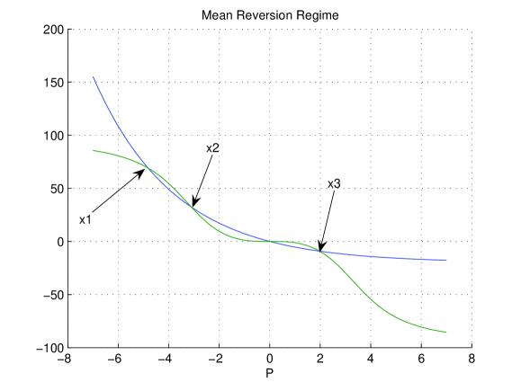
Figure 1 illustrates the mean reversion regime (the value of $P_{0}$ is set to be zero here). The region between points $x_{2}$ and $x_{3}$ on this figure is the range of values of $P$ where the mean reversion term dominates the social response function, as in (2). The parameter $\delta_{m}$ is the characteristic price scale of the mean reversion regime. Existence of such scale satisfying Assumption I’ follows from Assumption I since $\partial f(P_{0},P_{0})/\partial P=-\mu.$ Below we will sometimes consider $P_{0}$ depending on time. In that case, Assumption I’ holds at each $t$ with the corresponding $P_{0}(t).$

Our second assumption ensures existence of the bubble and collapse regimes.

Assumption II. Equation $\mu+x=\nu S(x)$ has exactly two positive roots, $x_{5}$ and $x_{6},$ and exactly one negative root, $x_{1}.$

It follows that equation $x=\nu S(x)$ has exactly two positive roots and exactly two negative roots, $x_{2}$ and $x_{3}$ (due to symmetry). The smaller of these positive roots will be denoted $x_{4}.$

Let us explain why Assumption II is relevant for the presence of the bubble regime. Intuitively, a sustained bubble is driven by the balance between social response function, growth in $P$ and the mean reversion term. For large values of $P,$ the mean reversion term is basically equal to $-\mu.$ Setting $P^{\prime}=x,$ and approximating $P(t)-P(t-1)\approx P^{\prime}(t)$, we arrive at the balance

(3) $$x+\mu=\nu S(x)$$

for the stable bubble regime. Given our assumptions on the structure of the response function $S,$ equation (3) can have two, one (this is a degenerate case) or zero positive roots. In the last two cases, the nonlinear response term is just too weak to sustain a bubble. Therefore, Assumption II is essentially just about the sufficient strength of the social response term. Observe that the smaller positive root, $x_{5},$ is unstable, while $x_{6}$ is stable (see Figure 2). The root $x_{6}$ then determines the asymptotic rate of growth in a bubble. The root $x_{5},$ on the other hand, determines the range of stability of the developed bubble regime (should a random fluctuation reduce the rate of growth below $x_{5},$ the bubble will puncture and collapse will likely begin). Let us set $\delta_{b}=(x_{6}-x_{5})/2$ – this parameter can be regarded as the typical stability scale of the bubble regime (it has dimension of price/time). Note that it is clear from the definition that $x_{5}>\delta_{m}.$

The positive root $x_{4}$ is relevant for values of $P$ not too far away from $P_{0}.$ When the mean reversion is small, $x_{4}$ is the threshold rate of growth for the start of the bubble. However, if the rate of growth will not accelerate quickly to beyond $x_{5},$ the beginning bubble may slow down and turn with the growth of $P$ – due to the mean reversion term getting stronger and approaching the value $-\mu.$

Figure 2.

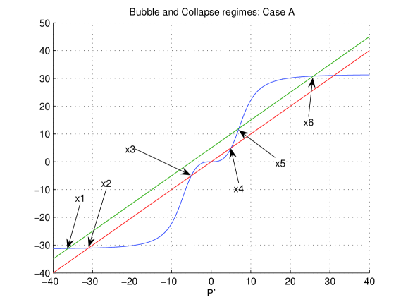
Similarly to $x_{6},$ the stable negative root $x_{1}$ determines the rate of collapse for large values of $P.$ The collapse regime is extremely stable for large $P.$ The system tends to go into a collapse with the rate of decay aproaching $x_{1}$ if only the rate of growth falls below $x_{5}$.

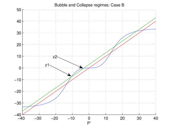
Observe that without Assumption II, under our structure assumptions on the function $S$ there is a possibility that (3) has three negative roots (or, in a degenerate case, two negative roots): see Figure 3 for illustration. In this case, the smaller (in absolute value) stable root $z_{2}$ determines the likely rate of decay right after the puncture of a bubble. We call such scenario ”a non-panic collapse”, since in many cases the primary driver of such decay is the mean reversion force that is close to the value $-\mu$, and the social response function $S$ does not play a big role. If $\mu$ is small, this regime may look like simply a pause in the bubble growth. A switch either into the bubble or into steeper collapse is possible if random fluctuations are present. Alternatively, the ”non-panic collapse” can simply bring the price all the way down to the equilibrium value $P_{0}$, and switch to the mean reversion regime. While this configuration is interesting and adds an extra phenomenon which deserves to be studied, in this paper we restrict ourselves to the simpler case covered by Assumption II: most collapses in practice tend to involve panic. The case with three negative roots will be studied elsewhere.

For values of $P$ closer to equilibrium, where $f(P,P_{0})$ cannot be regarded as just $-\mu,$ the stable negative root $x_{2}$ of $x=\nu S(x)$ approximates the rate of collapse decay. The unstable root $x_{3}$ provides a bound for the range of stability of the collapse (the collapse is definitely stable up to decay rates of $x_{3};$ it really is more stable since the mean reversion works in favor of collapse for values $P(t)>P_{0}$). We set $\delta_{c}=(x_{3}-x_{2})/2,$ and regard $\delta_{c}$ as the typical stability scale of the collapse regime. Let $a_{b}=x_{5}+\delta_{b}/2,$ and $a_{c}=x_{3}-\delta_{c}/2.$ Observe that

(4) $$\nu S(a_{b})-\mu-a_{b}=c_{b}\delta_{b}>0,$$

(5) $$\nu S(a_{c})-a_{c}=-c_{c}\delta_{c}<0,$$

where $c_{b},c_{c}>0$ are some fixed constants depending on $S.$ These inequalities, which follow from Assumption II, will be useful for us in the random case, where we will need some cushion to ensure the stability of the bubble and collapse regimes.

Figure 3.

We now describe the bubble and collapse regimes and their stability in the deterministic case.

The bubble regime. Assume that $P(t)-P(t-1)>x_{5}$ for all $t\in[t_{0}-1,t_{0}].$ Then we also have $P(t)-P(t-1)>x_{5}$ for all $t>t_{0}.$ Moreover, $P^{\prime}(t)\rightarrow x_{6}$ as $t\rightarrow\infty.$

Proof.

Assume, on the contrary, that there exists a time $t_{1}$ such that $P(t_{1})-P(t_{1}-1)=x_{5},$ and $t_{1}$ is the smallest such time greater than $t_{0}.$ However in that case, for every $t\in[t_{1}-1,t_{1}],$ we have

$$P^{\prime}(t)\geq-\mu+\nu S(P(t)-P(t-1))>-\mu+\nu S(x_{5})=x_{5}$$

due to Assumption II. It follows that $P(t_{1})-P(t_{1}-1)>x_{5}$, which is a contradiction. Hence, $P^{\prime}(t)>x_{5}$ and

(6) $$P(t)-P(t-1)>x_{5} t>t_{0}$$ for all .

Observe that, as a consequence, $P(t)\rightarrow\infty$ as $t\rightarrow\infty$. Let us denote

$$P_{n}={\rm min}_{t\in[t_{0}+n-1,t_{0}+n]}P(t),$$

then the sequence $P_{n}$ is increasing by (6), and, moreover, $P_{n}\geqslant C_{0}+nx_{5}$, with some constant $C_{0}$ that depends only on the data on the time interval $[t_{0}-1,t_{0}]$. We also define

$$p^{+}_{n}={\rm max}_{t\in[t_{0}+n-1,t_{0}+n]}P^{\prime}(t),$$

and

$$p^{-}_{n}={\rm min}_{t\in[t_{0}+n-1,t_{0}+n]}P^{\prime}(t).$$

We claim that

(7) $$\lim_{n\to\infty}p_{n}^{-}=\lim_{n\to\infty}p_{n}^{+}=x_{6}.$$

To this end we make the following observations. First, note that $p_{n}^{-}>x_{5}$ and $p_{n}^{+}>x_{5}$ for all $n$. We also claim that

(8) $$\hbox{if $p_{n}^{-}\leqslant x_{6}$ then $p_{n+1}^{-}\geqslant p_{n}^{-}$}.$$

Indeed, assume that $p_{n}^{-}\leqslant x_{6}$. For any $t\in[t_{0}+n,t_{0}+n+1]$ we have

(9) $$P^{\prime}(t)=-\mu+\mu e^{P_{0}-P}+\nu S(P(t)-P(t-1))>-\mu+\nu S(\min(p_{n}^{-},p_{n+1}^{-})),$$

thus

(10) $$p_{n+1}^{-}>-\mu+\nu S(\min(p_{n}^{-},p_{n+1}^{-})).$$

Now, if (8) fails then (10) implies that

(11) $$p_{n+1}^{-}>-\mu+\nu S(p_{n+1}^{-}).$$

As $p_{n+1}>x_{5}$ it follows from (11) that $p_{n+1}^{-}>x_{6}$, hence we have the inequalities

$$x_{6}\geqslant p_{n}^{-}\geqslant p_{n+1}^{-}>x_{6},$$

which is a contradiction. Thus, (8) holds.

Next, we show that

(12) if $$p_{k}^{-}\geqslant x_{6} p_{n}^{-}\geqslant x_{6} n\geqslant k$$ then for all .

It suffices to show that (12) holds for $n=k+1$. However, it follows from (10) that either

(13) $$p_{k+1}^{-}>-\mu+\nu S(p_{k}^{-})\geqslant-\mu+\nu S(x_{6})=x_{6},$$

or

(14) $$p_{k+1}^{-}>-\mu+\nu S(p_{k+1}^{-}),$$

which also implies that $p_{k+1}^{-}>x_{6}$. Therefore, (12) holds.

The next step is to show that there exists a constant $c_{0}$ so that

(15) if $$p_{n}^{+}\geqslant x_{6}+c_{0}e^{-nx_{5}} p_{n+1}^{+}\leqslant p_{n}^{+}$$ then .

Note that

$$p^{+}_{n+1}\leq-\mu+\mu e^{P_{0}-P_{n}}+\nu S(\max(p^{+}_{n},p_{n+1}^{+}))\leqslant-\mu+\mu e^{P_{0}-C_{0}}e^{-nx_{5}}+\nu S(\max(p^{+}_{n},p_{n+1}^{+})),$$

hence

(16) $$p^{+}_{n+1}\leq-\mu+d_{0}e^{-nx_{5}}+\nu S(\max(p^{+}_{n},p_{n+1}^{+})),$$

with $d_{0}=\mu\exp(P_{0}-C_{0})$. Now, if $p_{n}^{+}<p_{n+1}^{+}$ then

$$p^{+}_{n+1}\leq-\mu+d_{0}e^{-nx_{5}}+\nu S(p_{n+1}^{+}),$$

which, in turn, implies that

$$p_{n}^{+}<p_{n+1}^{+}<x_{6}+c_{0}e^{-nx_{5}}$$

with some constant $c_{0}$ that depends only on the behavior of the function $S(x)$ near $x=x_{6}$, and (15) follows.

Now, let us prove (7). Let us set

$$L^{+}=\limsup_{n\to\infty}p_{n}^{+}.$$

Passing to the limit in (16) gives

$$L^{+}\leqslant-\mu+\nu S(L^{+}),$$

hence $L^{+}\leqslant x_{6}$. Then (8) and (12) imply that

$$L^{-}=\lim_{n\to\infty}p_{n}^{-}$$

exists and $x_{5}<L^{-}\leqslant x_{6}$. Moreover, (10) implies that

$$L^{-}\geqslant-\mu+\nu S(L^{-}),$$

whence $L^{-}=x_{6}$. As $L^{+}\leqslant x_{6}$, and $L^{+}\geqslant L^{-}$, it follows that $L^{+}=x_{6}$ as well, and, moreover,

$$\liminf_{n\to\infty}p_{n}^{+}\geqslant\liminf_{n\to\infty}p_{n}^{-}=x_{6},$$

thus (7) holds. ∎

While the mean reversion and bubble regimes in the deterministic case continue indefinitely, the collapse regime ends once we reach the equilibrium value (in fact, as will be clear from the argument below, we should go well below the equilibrium value to break the decay).

The collapse regime. Assume that both $P(t)-P(t-1)<x_{3}$ and $P(t)>P_{0}$ for all $t\in[t_{0}-1,t_{0}].$ Then for any $t>t_{0}$ such that $P(s)$ remains larger than $P_{0}$ for all $t_{0}\leq s\leq t,$ we have $P(t)-P(t-1)<x_{3}.$ Moreover, if $P(t)>P_{0}$ for $t\in[t_{0}-1,t_{0}+1],$ and

$$x_{3}>{\rm max}_{t\in[t_{0}-1,t_{0}]}(P(t)-P(t-1))\equiv d_{0}>x_{2},$$

then the decay accelerates in the next time interval:

$${\rm max}_{t\in[t_{0},t_{0}+1]}(P(t)-P(t-1))\equiv d_{1}<d_{0}.$$

Remark. We lack a statement on the asymptotic rate of collapse since any collapse ends once $P_{0}$ is reached. But if one assumes that $P$ is very large in the beginning, one can prove that the rate of decay approaches $x_{1}$ while $P$ remains very large. The argument is similar to that given above in the bubble case.

Proof.

Suppose there exists $t_{1}>t_{0}$ such that for $t\in[t_{0},t_{1})$, we have $P(t)-P(t-1)<x_{3}$ and $P(t)>P_{0},$ but $P(t_{1})-P(t_{1}-1)=x_{3}.$ Then for any $t\in[t_{1}-1,t_{1}],$ we have

$$P^{\prime}(t)\leq\nu S(P(t)-P(t-1))<\nu S(x_{3})=x_{3},$$

giving us a contradiction.

Now let ${\rm max}_{t\in[t_{0}-1,t_{0}]}(P(t)-P(t-1))=d_{0},$ with $x_{2}<d_{0}<x_{3}.$ Then for every $t\in[t_{0}-1,t_{0}],$ we have $P^{\prime}(t)<\nu S(d_{0})<d_{0}$ by the definition of $x_{2}$ and $x_{3}.$ This implies, by a familiar argument, that $P(t)-P(t-1)<d_{0}$ for every $t\in[t_{0},t_{0}+1].$ ∎

It is clear that $P$ should fall sufficiently below $P_{0}$ to balance the speculative function. In particular, if the fall has been from large values of $P,$ we need at least $f(P,P_{0})\gtrsim x_{2}$ to break the fall.

We should stress that it is clear from our conditions that mean reversion, bubble and collapse do not exhaust the whole range of possible behaviors in our model. For most parameter ranges where the system does exhibit interesting behavior, there is a significant gap between mean reversion and bubble. We call it a transitory regime. In the random case, one situation where it appears is when a fluctuation kicks the price away from $P_{0}$ but not strongly enough for the bubble to form (for example, the rate of growth does not exceed $x_{4}>\delta_{m}$ or is just barely above it). In this regime, there is no dominating term. The effects of both mean reversion and social response may be significant. In the deterministic setting, what happens depends strongly both on the rate of growth and the value of $P$: for example, if $P>P_{0}$ and ${\rm max}_{t\in[t_{0}-1,t_{0}]}(P(t)-P(t-1))<x_{4},$ the growth will decelerate. In the random case, the evolution in the transitory regime becomes much more sensitive to randomness. The transitory regime is thus most difficult for rigorous analysis. In this paper, we will prove rigorous bounds on probabilities reflecting stability or transitions between mean reversion, bubble and collapse. The bounds we prove may be not quite sharp due to the transitory effects we just described.

Observe that in the deterministic case, the three basic regimes are not connected: one cannot transition between them, with the exception of the collapse regime which ends once the price has fallen enough. Other transitions will be made possible by randomness. There is a way, however, to ignite bubbles in the deterministic case as well – by adjusting the level of the equilibrium value, $P_{0}.$ This can be interpreted as a change in the fundamental data: a new positive earnings report in the case of a stock or a stimulative interest rate policy for real estate or fixed income investments. Since in practice, such change in $P_{0}$ often happens in a jump, that is what we will consider here. It is not difficult to adjust the arguments below to the case of a continuous dependence $P_{0}(t).$

The first observation is that if the jump in $P_{0}$ is small, then the bubble does not ignite.

Driving deterministic bubbles: a small jump. Assume that $|P(t)-P_{0}(t)|<\delta_{m}/2$ for $t\in[t_{0}-1,t_{0}],$ $P_{0}(t)=P_{-}.$ Assume also that $P_{0}$ jumps up at $t_{0}$ to a value $P_{+}$ and the size of the jump satisfies $0<P_{+}-P_{-}<\delta_{m}/2.$ Then we have $P(t)-P_{0}(t)<\delta_{m}/2$ and $P(t)-P_{0}(t)>-\delta_{m}$ for $t\in[t_{0},t_{0}+1],$ $P_{0}(t)=P_{+}.$ Thus we continue in the mean reversion regime for all future times.
Remark. We need a more relaxed lower bound above simply because the original bound may clearly fail right after the jump.

Proof.

Assume on the contrary that $P(t_{1})=P_{+}+\delta_{m}/2$ at some $t_{1}$ for the first time. Then we have

$$P^{\prime}(t_{1})=f(P_{+}+\delta_{m}/2,P_{+})+\nu S(P(t_{1})-P(t_{1}-1)),$$

and, moreover,

$$P(t_{1})-P(t_{1}-1)\leq P(t_{1})-P_{+}+P_{+}-P_{-}+P_{-}-P(t_{1}-1)\leq\delta_{m}/2+\delta_{m}/2+\delta_{m}/2=3\delta_{m}/2.$$

Using Assumption I’ with $x=\delta_{m}/2,$ gives

$$f(P_{+}+\delta_{m}/2,P_{+})+\nu S(3\delta_{m}/2)<0,$$

and so $P^{\prime}(t_{1})<0$ which is a contradiction. Similarly, assume that $P(t_{2})=P_{+}-\delta_{m}$ for some $t_{2}>t_{0}$ for the first time. But then

$$P^{\prime}(t_{2})=f(P_{+}-\delta_{m},P_{+})+\nu S(P_{+}-\delta_{m}-P(t_{2}-1))$$

$$\,\,\,\,\,\,\,\,\,\,\,\,\,\,\,\,\,\,\geq f(P_{+}-\delta_{m},P_{+})+\nu S(P_{+}-\delta_{m}-P_{-}-\delta_{m}/2)>0$$

by Assumption I’. ∎

On the other hand, a strong driving will necessarily lead to bubble ignition.

Driving deterministic bubbles: a large jump. Assume that $|P(t)-P_{0}(t)|<\delta_{m}/2$ for $t\in[t_{0}-1,t_{0}],$ $P_{0}(t)=P_{-}.$ Assume that $P_{0}$ jumps up at $t_{0}$ to a value $P_{+}$ and the size of the jump satisfies

$$P_{+}-P_{-}\geq x_{5}+\frac{x_{5}}{\mu}+\delta_{m}.$$

Then for all $t\in[t_{0}+1,t_{0}+2]$ we have $P(t)-P(t-1)>x_{5}.$

Proof.

First, observe that for all $t\in[t_{0},t_{0}+1]$ we have $P(t)-P(t-1)>-\delta_{m}.$ This is true since $P(t-1)\leq P_{-}+\delta_{m}/2$ by assumption, and $P(t)\geq P_{-}-\delta_{m}/2$ by the same argument as in the proof of stability of mean reversion regime (using $P_{+}>P_{-}$).

Now we claim that $P^{\prime}(t)>x_{5},$ for every $t\in[t_{0},t_{0}+1].$ Indeed, if $P(t)<P_{-}+x_{5}+\delta_{m}/2,$ then

$$P^{\prime}(t)>f(P(t),P_{+})+\nu S(-\delta_{m})=\mu(e^{P_{+}-P(t)}-1)-\mu(e^{\delta_{m}/2}-1).$$

We used Assumption I’ in the last step. Then

$$P^{\prime}(t)>\mu(P_{+}-P(t)-\delta_{m}/2)\geq x_{5}.$$

On the other hand, if $P(t)\geq P_{-}+x_{5}+\delta_{m}/2,$ then

$$P^{\prime}(t)>-\mu+\nu S(P(t)-P_{-}-\delta_{m}/2)\geq-\mu+\nu S(x_{5})\geq x_{5}.$$

Now we can prove that $P(t)-P(t-1)>x_{5}$ for all $t\in[t_{0}+1,t_{0}+2]$ by a familiar argument. Indeed, this is true for $t=t_{0}.$ Assuming existence of some minimal $t_{1}$ where we have $P(t_{1})-P(t_{1}-1)=x_{5},$ we quickly obtain a contradiction. ∎

3. The random case: heuristics

In this section, we will provide an intuitive picture of what to expect from our model (1) when the random term is included, but is small. This regime may be more relevant to modeling illiquid investments like real estate rather than liquid ones. Consider first the mean reversion regime. In this case we can regard the influence of the social response term as minor. It gets activated only once randomness, by accident, moves the price away from the mean reversion zone. Note that if we gradually drift away from $P_{0}$ – which is difficult due to mean reversion – we still do not activate the bubble regime as the social response term is small, but move into the transitory regime. Rather, we should have a jump of size $\sim a_{b}$ to enter the stable bubble regime. Let us set $P_{n}=P(t_{0}+n),$ $\Delta P_{n}=P_{n}-P_{n-1},$ $\Delta B_{n}=B_{n}-B_{n-1}.$ Then heuristically, the evolution of $P_{n}$ in mean reversion regime can be approximated by

$$\Delta P_{n}=\sigma\Delta B_{n}-\mu(P_{n}-P_{0}).$$

Intuitively, we pass into the stable bubble regime on the $n$th step if $\sigma\Delta B_{n}\gtrsim(1+\mu)a_{b}.$ Thus the probability $\lambda_{1}$ of bubble ignition at each step is roughly $1-\Phi(\frac{(1+\mu)a_{b}}{\sigma}),$ where $\Phi$ is the cumulative function of the normal distribution,

$$\Phi(x)=\frac{1}{\sqrt{2\pi}}\int_{-\infty}^{x}e^{-y^{2}/2}\,dy.$$

At this heuristic level, the dynamics in the mean reversion regime can be thought of as a Poisson-type process where on each time step we pass to the bubble regime with probability $\lambda_{1},$ and stay in the mean reversion regime with probability $1-\lambda_{1}.$ Of course, in reality the probability of bubble ignition depends on the past dynamics and on what exactly happens within the time interval. The social response term also increasingly plays a role as the system moves into the transitory regime which is more prone to creating bubbles than mean reversion. However, the above picture captures the most qualitative aspects of dynamics.

Once we are in the bubble regime, our rate of growth approaches $x_{6},$ and the bubble stability in terms of variations in the rate of growth is measured by $\delta_{b}.$ The dynamics is qualitatively described by

(17) $$\Delta P_{n}=-\mu+\sigma\Delta B_{n}+\nu S(\Delta P_{n-1}).$$

Now, in order for the bubble to burst and for dynamics to pass to the collapse regime, we need $\sigma\Delta B_{n}\gtrsim\delta_{b}.$ Thus, the dynamics in the bubble regime can be modeled by a Poisson-type process where on every time step we switch from bubble to collapse with the probability $\lambda_{2}\sim 1-\Phi(\delta_{b}/\sigma)$ and we stay in the bubble with the probability $1-\lambda_{2}.$ Observe the similarity between this heuristic picture and the well known simple discrete model proposed and investigated by Blanchard and Watson [5] (minus the no-arbitrage condition, which is not automatic in our model).

Finally, once we have entered the collapse regime, the dynamics in the leading order is described again by (17) (for larger values of $P,$ with the term $(-\mu)$ on the right side gradually disappearing as $P$ decreases). For large $P,$ the only way to break the collapse is to go back into the bubble regime, and for that one needs $\sigma\Delta B_{n}\gtrsim a_{b}-a_{c}.$ Observe that the probability of this is small compared to $\lambda_{1}$ and $\lambda_{2},$ due to $a_{b}>\delta_{b},$ $a_{c}<-\delta_{c}.$ As we approach the equilibrium value $P_{0},$ the condition for breaking the collapse gradually approaches $\sigma\Delta B_{n}\gtrsim\delta_{c},$ and the passage to the transitory or mean reversion regime becomes possible. Once we have broken through $P_{0},$ the push back to the mean generated by the mean reversion term increases rapidly. We pass from collapse to the recovery when $P_{0}-P\sim\log(1+\frac{\delta_{c}}{\mu}).$

We emphasize that the heuristic picture of this section cannot be expected to provide a close approximation of the real evolution in all possible relevant ranges of parameter values. For example, when the random term is sufficiently strong, transitory effects play an important role, and dependence of the evolution on details of the past dynamics increases notably. This regime is perhaps most interesting from the practical point of view. Still, in Section 6 devoted to numerical simulations, we will see that our heuristic picture appears to describe the evolution pretty well for a significant range of parameter values.

4. The Random Case: Mean Reversion, Bubble and Collapse

Now, we consider the full equation (1):

$$dP=f(P)dt+\sigma dB_{t}+\nu S(P(t)-P(t-1))dt.$$

Naturally, depending on the relative strength of parameters, this equation can exhibit very different behavior. For example, if both $\nu$ and $\sigma$ are small, the mean reversion term will always dominate and we will have a process very close to Ornstein-Uhlenbeck process. Taking $\sigma$ large emphasizes randomness, and then the nonlinear social response effects may be difficult to discern. In this section we provide rigorous analysis which is most relevant in the case of small to moderate random forcing. First, we describe the probabilistic stability of our basic regimes. For now, the equilibrium value $P_{0}$ is fixed.

Stability of the mean reversion regime. Assume that for all $t\in[t_{0}-1,t_{0}]$ we have $|P(t)-P_{0}|<\delta_{m},$ and $|P(t_{0})-P_{0}|<\delta_{m}/2.$ Then with probability at least $2\Phi(C\delta_{m}/\sigma)-1,$ we have that the same is true for $t\in[t_{0},t_{0}+1]:$ $|P(t)-P_{0}|<\delta_{m}$ for $t\in[t_{0},t_{0}+1]$ and $|P(t_{0}+1)-P_{0}|<\delta_{m}/2.$ Here $C>0$ is a universal constant.
Remark. A stronger condition at the end of the interval is necessary: if we had $|P(t_{0})-P_{0}|=\delta_{m},$ then we would have exited the interval $[P_{0}-\delta_{m},P_{0}+\delta_{m}]$ at later times with probability one.

Proof.

Let us assume that for any $t_{1}<t_{2}$, $t_{1},t_{2}\in[t_{0},t_{0}+1]$ we have

(18) $$\sigma|B_{t_{2}}-B_{t_{1}}|<{\rm min}(c_{m}\mu,1/4)\delta_{m},$$

where $c_{m}$ is the same as in Assumption I’. This is true in particular if

$$\sigma{\rm max}_{t_{0}\leq t\leq t_{0}+1}|B_{t}-B_{t_{0}}|<\frac{1}{2}{\rm min}(\mu c_{m},1/4)\delta_{m}.$$

The probability of this event is equal to $2\Phi(\frac{C\delta_{m}}{\sigma})-1.$

We claim that in this case, $|P(t)-P_{0}|\leq\delta_{m}$ for all $t\in[t_{0},t_{0}+1]$ and $|P(t_{0}+1)-P_{0}|<\delta_{m}/2.$ Let us verify that $P(t)\leq P_{0}+\delta_{m}$ for all $t\in[t_{0},t_{0}+1]$ and $P(t_{0}+1)<P_{0}+\delta_{m}/2.$ The other part of the condition can be verified similarly. Indeed, assume on the contrary that there exists $t_{3}$ with $P(t_{3})=P_{0}+\delta_{m}.$ Let $t_{4}$ be the largest time in $[t_{0},t_{1}]$ such that $P(t_{4})=P_{0}+\delta_{m}/2.$ Then we have

$$P(t_{3})-P(t_{4})=\int\limits_{t_{4}}^{t_{3}}(f(P(s),P_{0})+\nu S(P(s)-P(s-1)))\,ds+\sigma(B_{t_{3}}-B_{t_{4}}).$$

Note that due to $P(s-1)>P_{0}-\delta_{m}$ and Assumption I’, we have

$$f(P(s),P_{0})+\nu S(P(s)-P(s-1))<-c_{m}\mu\delta_{m}$$

for any $s$ in the interval of integration. Therefore we get

$$P(t_{3})-P(t_{4})<-c_{m}\mu\delta_{m}(t_{3}-t_{4})+\delta_{m}/4<\delta_{m}/4,$$

a contradiction to our choice of $t_{3},t_{4}.$

Similarly, under condition (18) we have $P(t_{0}+1)<P_{0}+\delta_{m}/2.$ Indeed, assume that $P(t_{0}+1)\geq P_{0}+\delta_{m}/2.$ If we ever have $P(t)<P_{0}+\delta_{m}/4$ for $t\in[t_{0},t_{0}+1],$ let $t_{3}$ be the largest time less than $t_{0}+1$ when $P(t_{3})=P_{0}+\delta_{m}/4.$ Then

$$P(t_{0}+1)-P(t_{3})=\int\limits_{t_{3}}^{t_{0}+1}(f(P(s),P_{0})+\nu S(P(s)-P(s-1)))\,ds+\sigma(B_{t_{0}+1}-B_{t_{3}})$$

$$\,\,\,\,\,\,\,\,\,\,\,\,\,\,\,\,\,\,\,\,\,\,\,\,\,\,\,\,\,\,\,\,\,\,\,\,\,\,\,\,\,\,\,\,\,\,\,<-c_{m}\mu\delta_{m}(t_{0}+1-t_{3})+\frac{\delta_{m}}{4}<\frac{\delta_{m}}{4},$$

which is a contradiction. We used Assumption I’ in estimating the integral. On the other hand, if $P(t)\geq P_{0}+\delta_{m}/4$ for all $t\in[t_{0},t_{0}+1]$ (but, as we saw above, $P(t)<P_{0}+\delta_{m}$), then

$$P(t_{0}+1)-P(t_{0})=\int\limits_{t_{0}}^{t_{0}+1}(f(P(s),P_{0})+\nu S(P(s)-P(s-1)))\,ds+\sigma(B_{t_{0}+1}-B_{t_{0}})$$

$$\,\,\,\,\,\,\,\,\,\,\,\,\,\,\,\,\,\,\,\,\,\,\,\,\,\,\,\,\,\,\,\,\,\,\,<-c_{m}\mu\delta_{m}+c_{m}\delta_{m}\mu=0,$$

once again a contradiction.

Thus, under our condition on the maximum of Brownian motion, the mean reversion regime is preserved. ∎

Stability of the bubble regime. Assume that for $t\in[t_{0}-1,t_{0}],$ we have $P(t)-P(t-1)>a_{b},$ and $\sigma{\rm max}_{t\in[t_{0}-1,t_{0}]}|B_{t}-B_{t_{0}-1}|<c_{b}\delta_{b}/4.$ Then with probability at least $2\Phi(C\delta_{b}/\sigma)-1,$ the same is true for $t\in[t_{0},t_{0}+1]$ (but $t_{0}-1$ is replaced by $t_{0}$).

Proof.

Suppose that for any $t_{1}<t_{2},$ $t_{1},t_{2}\in[t_{0},t_{0}+1]$ we have $\sigma(B_{t_{2}}-B_{t_{1}})>-c_{b}\delta_{b}/2.$ This is true with probability ta least $2\Phi(C\delta_{b}/\sigma)-1.$ Let us show that in this case,

$$P(t)-P(t-1)>a_{b} t\in[t_{0},t_{0}+1].$$ for all

This holds for $t_{0}$ by our assumption. Let $t_{1}$ be the first time when $P(t_{1})-P(t_{1}-1)=a_{b}.$ Then

$$P(t_{1})-P(t_{1}-1)\geq-\mu+\nu S(a_{b})+\sigma(B_{t_{1}}-B_{t_{1}-1})>a_{b}$$

under the assumption on Brownian motion and (4). This is a contradiction. ∎

Remark. We need an extra assumption on the behavior of Brownian motion during the past interval $[t_{0}-1,t_{0}]$ since there are some unlikely scenarios where, due to Brownian motion, we essentially set up the exit from the bubble regime during $[t_{0}-1,t_{0}]$ even though $P(t)-P(t-1)$ stays large for this time interval.

Stability of the Collapse regime. Assume that $P(t)-P(t-1)<a_{c}$ and $P(t)>P_{0}$ for $t\in[t_{0}-1,t_{0}].$ Assume also that $\sigma{\rm max}_{t\in[t_{0}-1,t_{0}]}|(B_{t}-B_{t_{0}-1}|\geq c_{c}\delta_{c}/4.$ Then with probability at least $2\Phi(C\delta_{c}/\sigma)-1$ either there exists a time $t\in[t_{0},t_{0}+1]$ so that $P(t)<P_{0}$ ,or $P(t)-P(t-1)<a_{c}$ for all $t\in[t_{0},t_{0}+1]$.

Proof.

Let us assume that for any $t_{1}<t_{2},$ $t_{1},t_{2}\in[t_{0},t_{0}+1]$ we have $\sigma(B_{t_{2}}-B_{t_{1}})<c_{c}\delta_{c}/2.$ This is true with probability exceeding $2\Phi(C\delta_{c}/\sigma)-1.$ Assume, on the contrary, that $P(t)>P_{0}$ for all $t\in[t_{0},t_{0}+1],$ but there exists $t_{1}$ such that $P(t_{1})-P(t_{1}-1)=a_{c}.$ But then

$$P(t_{1})-P(t_{1}-1)\leq\nu S(a_{c})+\sigma(B_{t_{1}}-B_{t_{1}-1})\leq a_{c}-c_{c}\delta_{c}+c_{c}\delta_{c}/2<a_{c},$$

which is a contradiction. ∎

As in the previous case, it is easy to construct a scenario showing that we need to assume something about the Brownian motion on the interval $[t_{0}-1,t_{0}]$ in order to obtain a reasonable bound on the probability of the continuation of the collapse regime.

Next, we look at a new phenomenon which appears in our model due to randomness.

The bubble ignition probability. Assume that for $t\in[t_{0}-1,t_{0}],$ we have $|P(t)-P_{0}|<\delta_{m},$ and $|P(t_{0})-P_{0}|<\delta_{m}/2.$ Then with a positive probability exceeding

(19) $$p_{0}=e^{-(a_{b}+2\mu+\delta_{m}+c_{b}\delta_{b})^{2}/\sigma^{2}}\left(2\Phi\left(\frac{{\rm min}(\delta_{m},c_{b}\delta_{b})}{4\sigma}\right)-1\right)\left(2\Phi\left(\frac{c_{b}\delta_{b}}{8\sigma}\right)-1\right),$$

we have $P(t)-P(t-1)>a_{b}$ for all $t\in[t_{0}+1,t_{0}+2].$ Here $c_{b}$ is as in (4).

Proof.

We will identify just one scenario leading to bubble ignition, and will estimate its probability. Assume that

(20) $$|\sigma(B_{t}-B_{t_{0}})-(a_{b}+2\mu+\delta_{m}+c_{b}\delta_{b})(t-t_{0})|\leq\frac{{\rm min}(\delta_{m},c_{b}\delta_{b})}{4},$$

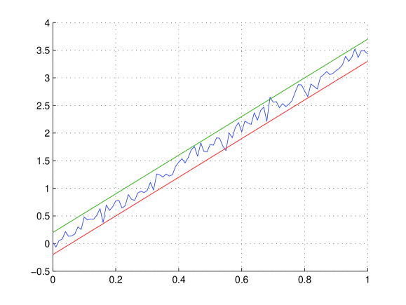
for all $t\in[t_{0},t_{0}+1]$ (one sample path satisfying this bound appears on Figure 4).

Figure 4. One possible behavior of the Brownian motion leading to the bubble ignition

We will estimate the probability of (20) in Lemma 1 below. First, we claim that under assumption (20), we have $P(t)-P(t-1)>-2\delta_{m}$ for all $t\in[t_{0},t_{0}+1].$ This follows from $P(t-1)\leq P_{0}+\delta_{m}$ due to our assumptions, and from $P(t)\geq P_{0}-\delta_{m}.$ The latter inequality can be established, given (20), similarly to the proof of the stability of random mean reversion regime.

Secondly, we claim that $P(t_{0}+1)-P(t_{0})>a_{b}.$ Indeed,

$$P(t_{0}+1)-P(t_{0})>-\mu+\sigma(B_{t_{0}+1}-B_{t_{0}})+\nu S(-2\delta_{m}).$$

Observe that due to Assumption I’, $\nu S(-2\delta_{m})=-\nu S(2\delta_{m})>-\mu.$ Then using (20), we obtain

$$P(t_{0}+1)-P(t_{0})>-2\mu+(a_{b}+2\mu+\delta_{m}+c_{b}\delta_{b})-\frac{{\rm min}(\delta_{m},c_{b}\delta_{b})}{2}>a_{b}.$$

Finally, assume that $P(t_{1})-P(t_{1}-1)=a_{b}$ for the first time at some $t_{1}\in[t_{0}+1,t_{0}+2].$ Let us split

$$P(t_{1})-P(t_{1}-1)=P(t_{1})-P(t_{0}+1)+P(t_{0}+1)-P(t_{1}-1).$$

Then

$$P(t_{1})-P(t_{0}+1)\geq-\mu(t_{1}-t_{0}-1)+\sigma(B_{t_{1}}-B_{t_{0}+1})+\nu S(a_{b})(t_{1}-t_{0}-1)$$

$$>(a_{b}+c_{b}\delta_{b})(t_{1}-t_{0}-1)+\sigma(B_{t_{1}}-B_{t_{0}+1}).$$

We used (4) in the second step. Assume that for any $t_{2}<t_{3},$ $t_{2},t_{3}\in[t_{0}+1,t_{0}+2]$ we have $\sigma(B_{t_{3}}-B_{t_{2}})>-c_{b}\delta_{b}/4.$ This happens with probability exceeding $2\Phi\left(\frac{c_{b}\delta_{b}}{8\sigma}\right)-1.$ Then

(21) $$P(t_{1})-P(t_{0}+1)\geq(a_{b}+c_{b}\delta_{b})(t_{1}-t_{0}-1)-c_{b}\delta_{b}/4.$$

Next,

$$P(t_{0}+1)-P(t_{1}-1)\geq-\mu(t_{0}+2-t_{1})+\sigma(B_{t_{0}+1}-B_{t_{1}-1})+\nu\int\limits_{t_{1}-1}^{t_{0}+1}S(P(t)-P(t-1))\,dt$$

$$\geq-2\mu(t_{0}+2-t_{1})+(2\mu+a_{b}+\delta_{m}+c_{b}\delta_{b})(t_{0}+2-t_{1})-\frac{{\rm min}(\delta_{m},c_{b}\delta_{b})}{2}\geq$$

(22) $$\geq(a_{b}+\delta_{m}+c_{b}\delta_{b})(t_{0}+2-t_{1})-\frac{{\rm min}(\delta_{m},c_{b}\delta_{b})}{2}.$$

Adding up (21) and (22), we obtain

$$P(t_{1})-P(t_{1}-1)>a_{b}+c_{b}\delta_{b}/4>a_{b},$$

and this is a contradiction.

It remains to estimate the probability of (20).

Lemma 1.

Let $X_{t}=B_{t}-ct.$ Then

(23) $$P({\rm max}_{0\leq s\leq t}|X_{s}|\leq b)\geq e^{-cb-\frac{c^{2}t}{2}}(2\Phi(b/\sqrt{t})-1).$$

Proof.

The proof is a simple application of the Girsanov theorem. Let $A$ be the set of paths where ${\rm max}_{0\leq s\leq t}|X_{s}|\leq b.$ Let $Z_{t}=e^{cB_{t}-\frac{c^{2}t}{2}},$ and define a new measure $dQ_{t}=Z_{t}dP_{t}.$ Then by Girsanov’s theorem, $X_{t}$ is a Brownian motion with respect to $dQ_{t}$, hence $Q(A)\geq 2\Phi(b/\sqrt{t})-1.$ Denote by $\chi_{A}$ the characteristic function of this set, and by ${\mathbb{E}}_{Q}$ the expectation taken with respect to the measure $dQ.$ Then

$$P(A)={\mathbb{E}}_{Q}[e^{-cB_{t}+\frac{c^{2}t}{2}}\chi_{A}]\geq{\mathbb{E}}_{Q}[e^{-c(ct+b)+\frac{c^{2}t}{2}}\chi_{A}]=e^{-cb-\frac{c^{2}t}{2}}Q(A).$$

We used that on $A,$ $B_{t}\leq ct+b.$ Thus,

$$P(A)\geq e^{-cb-\frac{c^{2}t}{2}}\left(2\Phi(b/\sqrt{t})-1\right).$$

∎

It follows from Lemma 1 that the probability of (20) satisfies

$$P\left({\rm max}_{0\leq s\leq 1}\left|B_{s}-\frac{a_{b}+2\mu+\delta_{m}+c_{b}\delta_{b}}{\sigma}s\right|\leq\frac{{\rm min}(\delta_{m},c_{b}\delta_{b})}{4\sigma}\right)\geq$$

$$e^{-(a_{b}+2\mu+\delta_{m}+c_{b}\delta_{b})^{2}/\sigma^{2}}\left(2\Phi\left(\frac{{\rm min}(\delta_{m},c_{b}\delta_{b})}{4\sigma}\right)-1\right)$$

(observe that the $cb$ term in the exponent in (23) is dominated by $c^{2}t/2$ in our case). Multiplying it by the probability of an independent Brownian motion behavior we required on $[t_{0}+1,t_{0}+2]$ leads to (19). ∎

Next, we look at the probability of the bubble regime switching to a collapse.

The bubble collapse probability. Assume that we are in a Bubble regime: for $t\in[t_{0}-1,t_{0}],$ $P(t)-P(t-1)>a_{b}$ and $P(t)>P_{0}.$ Then with probability exceeding

(24) $$e^{-(\nu-a_{c}+c_{c}\delta_{c})^{2}/\sigma^{2}}\left(2\Phi\left(\frac{c_{c}\delta_{c}}{8\sigma}\right)-1\right)\left(2\Phi\left(\frac{{\rm min}(\delta_{m},c_{b}\delta_{b})}{4\sigma}\right)-1\right)$$

we have either $P(t)\leq P_{0}$ for some $t\in[t_{0},t_{0}+2],$ or $P(t)-P(t-1)<a_{c}$ for all $t\in[t_{0}+1,t_{0}+2].$

Proof.

The argument is similar to the bubble ignition case, and we leave it to the interested reader to complete it. ∎

One of the debatable features of the bubble equation is that the bubble to collapse transition probability does not appear to increase with growth of $P.$ In fact, there is a slight increase due to decay in $f(P,P_{0}),$ but it is likely that the effect is insignificant when $\nu\gg\mu.$ In the discussion section we propose a slightly more complex model that is much more sensitive to the level of $P.$ The drawback is the presence of an additional parameter controlling the negative feedback response to growth in price. Given how hard this parameter is to estimate in practice, we believe there is some merit in keeping things simple and elegant as in the bubble equation, where the timing of collapse is purely random.

5. The Random Case: Forcing a Bubble

In this section, we consider the random case with a changing $P_{0}.$

Driving random bubbles: a small jump. Assume that for all $t\in[t_{0}-1,t_{0}],$ we have $|P(t)-P_{0}(t)|<\delta_{m},$ $|P(t_{0})-P_{0}(t)|<\delta_{m}/2$ where $P_{0}(t)=P_{-}.$ Assume that at $t_{0}$ the stable value $P_{0}$ undergoes a jump up to $P_{+},$ with $P_{+}-P_{-}<\delta_{m}/4$, and $P_{0}(t)$ stays equal to $P_{+}$ after that. Then with probability at least $2\Phi(C\delta_{m}/\sigma)-1,$ we have $|P(t)-P_{+}|<\delta_{m}$ for $t\in[t_{0},t_{0}+1],$ and $|P(t_{0}+1)-P_{+}|<\delta_{m}/2.$

Proof.

Let us estimate the probability of $P(t)\geq P_{+}-\delta_{m}$ for $t\in[t_{0},t_{0}+1]$ and $P(t_{0}+1)\geq P_{+}-\delta_{m}/2.$ The other half of the statement is similar and is in fact a bit easier since there is more danger in violating the lower boundary due to the increase in $P_{0}.$ Similarly to the stability argument without change in $P_{0},$ assume that $\sigma|B_{t_{3}}-B_{t_{2}}|<{\rm min}(c_{m}\mu,1/4)\delta_{m}$ for any $t_{3}>t_{2},$ $t_{2},t_{3}\in[t_{0},t_{0}+1].$ The probability of this exceeds $2\Phi\left(\frac{\delta_{m}}{8\sigma}\right)-1.$ Assume that there exists $t_{1}$ such that $P(t_{1})-P_{+}=-\delta_{m},$ and look at the minimal such $t_{1}.$ Since $P(t_{0})-P_{+}>-3\delta_{m}/4,$ find the largest $t_{4}\in[t_{0},t_{1}]$ such that $P(t_{4})-P_{+}=-3\delta_{m}/4.$ Consider

(25) $$P(t_{1})-P(t_{4})=\int\limits_{t_{4}}^{t_{1}}f(P(t),P_{+})\,dt+\nu\int\limits_{t_{4}}^{t_{1}}S(P(t)-P(t-1))\,dt+\sigma(B_{t_{1}}-B_{t_{4}}).$$

Observe that

$$P(t)-P(t-1)\geq P(t)-P_{+}+P_{+}-P_{-}-\delta_{m}/2\geq P(t)-P_{+}-3\delta_{m}/4.$$

Then by Assumption I’, we have

$$f(P(t),P_{+})+\nu S(P(t)-P(t-1))\geq c_{m}\mu\delta_{m}$$

in (25). Given our Brownian motion assumption, we obtain

$$P(t_{1})-P(t_{4})\geq-\delta_{m}/4+c_{m}\mu\delta_{m}(t_{1}-t_{4})>-\delta_{m}/4,$$

a contradiction.

Next, assume that $P(t_{0}+1)<P_{+}-\delta_{m}/2.$ If we ever have $P(t)>P_{+}-\delta_{m}/4$ in $[t_{0},t_{0}+1],$ let $t_{5}$ be the largest time where we have $P(t_{5})=P_{+}-\delta_{m}/4.$ Then

$$P(t_{0}+1)-P(t_{5})=\int_{t_{5}}^{t_{0}+1}(f(P(s),P_{+})+\nu S(P(s)-P(s-1)))\,ds+$$

$$\sigma(B_{t_{0}+1}-B_{t_{5}})\geq c_{m}\mu\delta_{m}(t_{0}+1-t_{5})-\delta_{m}/4,$$

giving a contradiction. We used Assumption I’ in the second step. In the case if $P(t)<P_{+}-\delta_{m}/4$ (but we saw $P(t)>P_{+}-\delta_{m}$) for all $t\in[t_{0},t_{0}+1],$ we have

$$P(t_{0}+1)-P(t_{0})\geq c_{m}\mu\delta_{m}-c_{m}\mu\delta_{m}>0,$$

contradiction. ∎

Now we consider the probability of bubble ignition given a strong jump in $P_{0}.$
Driving random bubbles: a large jump. Assume that for all times $t\in[t_{0}-1,t_{0}]$ we have $|P(t)-P_{0}(t)|<\delta_{m},$ and $|P(t_{0})-P_{0}(t_{0})|<\delta_{m}/2,$ with $P_{0}(t)=P_{-}.$ Assume that at $t=t_{0}$ $P_{0}$ jumps to a value $P_{+},$ and the size of jump satisfies

(26) $$P_{+}-P_{-}\geq\frac{2a_{b}+3\delta_{m}}{{\rm min}(\mu,1)}.$$

Then with probability exceeding $2\Phi(C{\rm min}(\delta_{m},c_{b}\delta_{b})/\sigma)-1,$ we have $P(t)-P(t-1)>a_{b}$ for all $t\in[t_{0}+1,t_{0}+2].$

Proof.

The main step in the proof is the following claim. Suppose, in addition to the assumptions above, that for any $t_{2},t_{3}\in[t_{0},t_{0}+1],$ $t_{3}>t_{2},$ we have

(27) $$\sigma(B_{t_{3}}-B_{t_{2}})>-{\rm min}(\delta_{m},c_{b}\delta_{b})/2.$$

Then

(28) $$P(t_{3})-P(t_{2})>(a_{b}+{\rm min}(\delta_{m},c_{b}\delta_{b}))(t_{3}-t_{2})-{\rm min}(\delta_{m},c_{b}\delta_{b})/2.$$

To prove (28), first observe that under our assumptions $P(t)-P(t-1)>-2\delta_{m}$ for all $t\in[t_{0},t_{0}+1].$ This can be verified using (27) similarly to the proof of stability in random mean reversion regime. Now

(29) $$P(t_{3})-P(t_{2})=\int_{t_{2}}^{t_{3}}\left(f(P(t),P_{+})+\nu S(P(t)-P(t-1))\right)\,dt+\sigma(B_{t_{3}}-B_{t_{2}}).$$

If, on the other hand, $P(t)-P_{-}>a_{b}+\delta_{m},$ then $P(t)-P(t-1)>a_{b}$ and therefore $\nu S(P(t)-P(t-1))>a_{b}+c_{b}\delta_{b}+\mu.$ Since $f(P(t),P_{+})>-\mu$ for all values of $P(t),$ we find that the expression under integral in (29) is greater then $a_{b}+c_{b}\delta_{b}.$ Now if $P(t)-P_{-}\leq a_{b}+\delta_{m},$ then by (26) we have

$$P_{+}-P(t)>\frac{a_{b}+2\delta_{m}}{{\rm min}(\mu,1)}.$$

In this case the expression under integral in (29) exceeds

$$\mu\left(e^{\frac{a_{b}+2\delta_{m}}{{\rm min}(\mu,1)}}-1\right)+\nu S(-2\delta_{m})\geq\mu\left(e^{\frac{a_{b}+2\delta_{m}}{{\rm min}(\mu,1)}}-e^{\delta_{m}}\right)\geq\mu\frac{a_{b}+\delta_{m}}{{\rm min(\mu,1)}}>a_{b}+\delta_{m}.$$

Here in the first step we used $\nu S(-2\delta_{m})>\mu(1-e^{\delta_{m}}),$ which follows from Assumption I’. Combining these estimates and assumption (27) leads to (28).

Next, suppose that the Brownian motion on the interval $[t_{0}+1,t_{0}+2]$ satisfies

(30) $$\sigma(B_{t_{3}}-B_{t_{2}})>-c_{b}\delta_{b}/2$$

for any $t_{3},t_{2}\in[t_{0}+1,t_{0}+2],$ $t_{3}>t_{2}.$ Observe that (28) implies that $P(t_{0}+1)-P(t_{0})>a_{b}.$ Let us show that the inequality persists for all $t\in[t_{0}+1,t_{0}+2]$ given (30). Assume, on the contrary, that $t_{1}\in[t_{0}+1,t_{0}+2]$ is the minimal time such that $P(t_{1})-P(t_{1}-1)=a_{b}.$ Split $P(t_{1})-P(t_{1}-1)=P(t_{1})-P(t_{0}+1)+P(t_{0}+1)-P(t_{1}-1).$ Then

$$P(t_{1})-P(t_{0}+1)>(\nu S(a_{b})-\mu)(t_{1}-t_{0}-1)+\sigma(B_{t_{1}}-B_{t_{0}+1})>(a_{b}+c_{b}\delta_{b})(t_{1}-t_{0}-1)-c_{b}\delta_{b}/2.$$

On the other hand, (28) implies that

$$P(t_{0}+1)-P(t_{1}-1)>(a_{b}+{\rm min}(\delta_{m},c_{b}\delta_{b}))(t_{0}+2-t_{1})-{\rm min}(\delta_{m},c_{b}\delta_{b})/2.$$

Combining these two estimates, we find that $P(t_{1})-P(t_{1}-1)>a_{b}$ - contradiction.

It remains to observe that the probability of both (27) and (30) happening can be estimated from below by $2\Phi\left(\frac{{\rm min}(\delta_{m},c_{b}\delta_{b})}{2\sqrt{2}\sigma}\right)-1.$ ∎

6. Numerical Simulations

We have tested the bubble equation dynamics on a wide range of parameter values. The Matlab random number generator was used for simulations. The model seems to be quite robust to the type of random forcing: mean zero uniformly distributed and normally distributed random terms with comparable variances lead to very similar results. This is again to be expected from the analytical point of view, since the properties of the Brownian motion used in the proofs are fairly generic and shared by many other random processes. The simulations were performed with the nonlinear response term $S(x)=\arctan(dx^{2n+1}),$ with $n=1,2$ or $3$ and $d$ a varying parameter. The roots $x_{i},$ $i=1,...6$ were computed for each parameter set tried. When clear bubble and collapse regimes were observable, the rates of growth and decay showed very good agreement with the ones predicted by values of the relevant roots.

As one can expect, the behavior of the model depends strongly on the balance between different parameters. First of all, if we want to observe bubbles, we should set $\nu\gtrsim\mu$. We found three distinct regimes for the Bubble equation.

Figure 5. Big rare bubbles phase: $\nu\gtrsim\mu\gtrsim\sigma^{2}$

Figure 6. Big rare bubbles phase: $\nu\gtrsim\mu\gtrsim\sigma^{2}$: Serial bubbles.

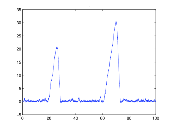
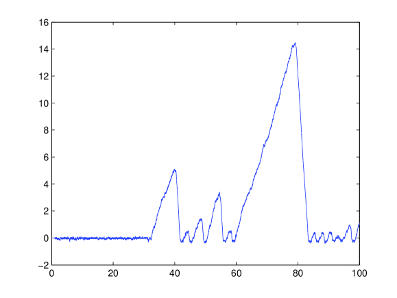
Regime 1: $\nu\gtrsim\mu\gtrsim\sigma^{2}$, or big rare bubbles regime. The three regimes described in analytical part of the paper are very clear cut here. Transitions are relatively rare. The heuristic picture of Section 3 seems to apply very well. A typical simulation is shown on Figure 5. In this regime, we noted that the likelihood of serial bubbles occurence, passing from complete collapse right to the next bubble, may be significant. This happens if the price compression below $P_{0}$ (which according to the heuristics is of the order $\sim\log\left(1+\frac{\delta_{c}}{\mu}\right)$) is comparable to $x_{5}.$ In that case the recovery to $P_{0}$ level provides enough of a trend to help ignite the next bubble (see Figure 6). The run on Figure 5 corresponds to $\nu=5,$ $\mu=4,$ $\sigma=3,$ $S$ cubic with $d=0.4.$ This corresponds to $x_{1}\sim-12,$ $x_{2}\sim-7.5,$ $x_{3}\sim-0.5,$ $x_{4}\sim 0.5,$ $x_{5}\sim 2,$ $x_{6}\sim 3,$ and $\delta_{m}\sim 1.$ It is clear from these values that the stability of the mean reversion and bubble regimes is actually even stronger than one can expect from our analytical bounds. In fact, taking smaller $\sigma$ usually led to very long mean reversion runs, followed by eventual bubbles which grew huge and exceeded our computer capacity before collapsing.

The fact that the dynamics in big rare bubbles regime is described quite well by heuristics of Section 3 makes it also close to the well known bubble model of Blanchard and Watson [5]. It would be of interest to show that under certain scaling assumptions, the dynamics of the bubble equation converges in the rigorous sense to a Poisson-type process with just three regimes of constant, exponential growth and exponential collapse.

Figure 7. Strong randomness phase: $\sigma^{2}\gtrsim\nu\gtrsim\mu$

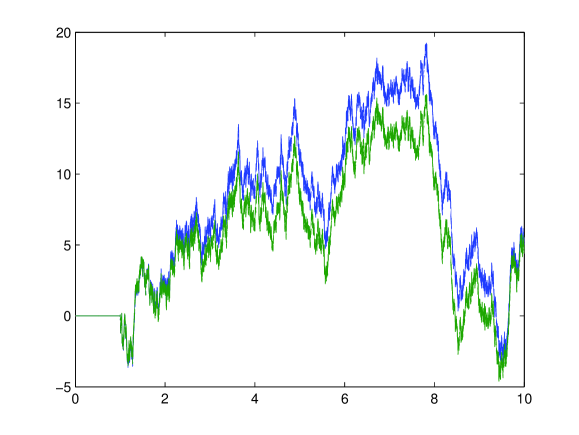
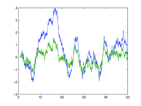
Regime 2: $\sigma^{2}\gtrsim\nu\gtrsim\mu$, or strong randomness regime. In this phase the effects of the social response term are weak compared to random fluctuations. The mean reversion, bubble and collapse regimes are difficult to isolate, and the dynamics is far from the heuristic model of Section 3. A sample simulation of this regime is shown on Figure 7. One graph is the price evolution given by the bubble equation, and the other, provided for comparison, is the dynamics corresponding to $\nu=0$ (and so it is just an Ornstein-Uhlenbeck process).

The bubble equation price tends to overshoot Ornstein-Uhlenbeck, but fairly slightly, and there is no sustained bubble regime. The parameters are $\nu=0.6,$ $\mu=0.2,$ $\sigma=20,$ the function $S$ is quintic with $d=90.$

Figure 8. The balanced phase: $\sigma\sim\nu\gtrsim\mu$

Figure 9. The balanced phase: stronger randomness

Figure 10. A small jump in fundamentals: no bubble ignition

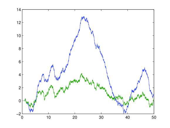
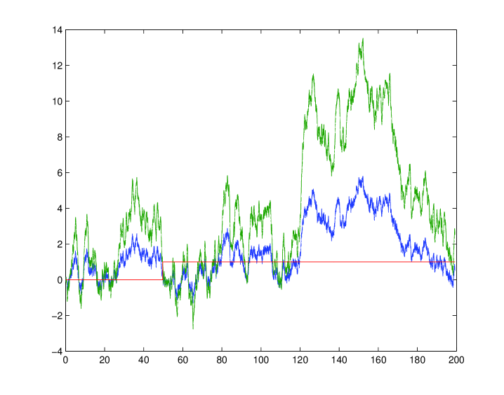
Regime 3. The most interesting phase appears to be when $\sigma$ is slightly larger or comparable to $\nu$, and $\mu$ is also comparable or weaker. It appears that this is the parameter range that is most likely to be relevant in most applications with liquid instruments. Here one can still sometimes distinguish the different regimes (although mean reversion is very unstable if $\mu$ is small). Yet transitory effects are stronger than in big rare bubbles phase. Figures 8 and 9 show some typical runs in this regime. As before, the Ornstein-Uhlenbeck process corresponding to the same random sample but with $\nu=0$ is graphed for comparison.

Figure 8 corresponds to $\nu=0.6,$ $\mu=0.23$ and $\sigma=2.$ The function $S$ is quintic, with $d=90.$ The Figure 9 corresponds to $\nu=0.42,$ $\mu=0.15,$ $\sigma=2,$ $S$ is cubic with $d=90.$

Figure 9 corresponds to relatively stronger randomness. While the nonlinear effects are still strong, fairly long transitory regimes become possible. Figure 8 shows an interesting phenomenon of a collapse regime switching back into bubble significantly above $P_{0}.$ It is clear by looking at the corresponding Ornstein-Uhlenbeck process graph that randomness drives these switches. In both simulations, social response term increases the effective volatility of dynamics, stronger on the upside (creating bubbles) but also on the downside after collapse (this difference in the strength of the effect has clearly to do with very quick growth of the mean reversion function once the price is below $P_{0}$).

Figure 11. A large jump in fundamentals causes bubble ignition

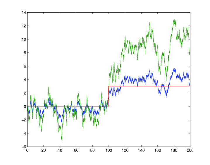
Next we investigate the likelihood of a jump in fundamentals igniting a bubble. We find that the probability of the bubble ignition becomes significant if the jump becomes comparable in size to $\nu.$ The Figure 10 shows a simulation where the jump does not cause a bubble, while Figure 11 shows a larger jump causing a bubble to ignite. On both figures, $P(t),$ $P_{0}(t)$ and the Ornstein-Uhlenbeck process corresponding to $\nu=0$ case are graphed.

Figure 12. The balanced phase: varying $P_{0}$

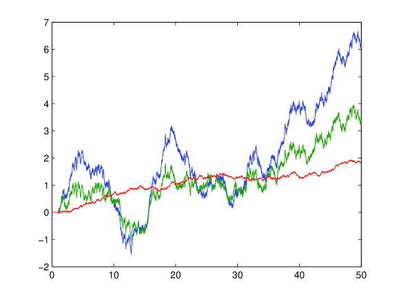
The final graph shows a simulation where the stable value $P_{0}$ depends on time (Figure 12). The particular model we used is a random walk with a drift; the volatility of $P_{0}$ is much lower than that of $P.$ All other parameters of the bubble equation are the same as in the run corresponding to Figure 9. The graphs on Figure 12 are those of $P_{0}(t),$ $P(t)$ and the corresponding Ornstein-Uhlenbeck process.

7. Discussion and Further Directions

The main goal of this paper was to present a simple differential equations model of the effects of human psychology in asset pricing. We tried to keep the model as simple as possible conditioned on the fact that it should exhibit sufficiently rich set of behaviors. A very interesting question that we did not address in this paper is the statistical properties of price returns generated by (1). It is well known that empirical daily price returns of various financial instruments such as for example major indexes demonstrate deviations from normal distribution, in particular power-like tails in the distribution of the returns. Typically, lack of strong correlations in the ACF of daily returns is observed (even though for some indexes and for some historical periods significant correlation can be present (see e.g. [33]). On the other hand, the volatility of returns exhibits clustering with ACF decaying at a slow power rate. A number of models have been proposed that can fairly accurately account for these statistical properties (see e.g. [37, 18, 47], and also [41, 45] for reviews). These models, however, tend to be more sophisticated than the one considered here. Can one obtain similar results for a simpler model (1)? It is likely that some modifications will be needed, in particular to reduce correlations in the return series. We plan to discuss the statistical properties of the model and some of its modifications in a future publication.

Another possible future direction of research involves bubble formation in spatially distributed systems, such as the real estate markets. The price is now a function of both space and time, $P(x,t).$ In the simplest case, the problem can be set on a graph, where each vertex $v_{j},$ $j=1,\dots,N$ corresponds to a town or a city. The interaction between prices $p_{i}$ and $p_{j}$ in cities $v_{i}$ and $v_{j}$ is defined by a diffusion coefficient $\kappa_{ij}.$ This coefficient models the degree of contact these cities have, geographical proximity and generally the degree to which the real estate prices in one city are likely to influence the prices in the other. To each $v_{i}$ we also assign a number $q_{i},$ which measures the size of $v_{i}$’s market. In addition, the stable value $p^{0}_{i}$ varies from city to city. Then one possible model for price dynamics is given by

$$dp_{i}(t)=\sum_{j=1}^{N}\kappa_{ij}(p_{i}-p_{j})\frac{1}{a_{j}}+f(p_{i},p^{0}_{i})+\sigma dB^{i}_{t}+\nu S(p_{i}(t)-p_{i}(t-1)).$$

The relative simplicity of the equation (1) describing price in every graph vertex (city) makes the model look approachable. Some of the interesting questions to study in this case are possibility and likelihood of bubble contagion (or bubble front propagation) doe to price diffusion, or possibility of existence of localized bubbles.

Yet another interesting problem is suggested by numerical simulations in the big rare bubbles regime. Is it true that under certain scaling assumptions, the equation (1) can be rigorously shown to converge to a nontrivial limit, such as suggested in Section 3? Does one get simply three possible clear cut regimes with Poisson-like switching between them? A result like that would establish an analytical link between relatively sophisticated bubble equation and simpler discrete bubble models reminiscent of the one appearing in Blanchard-Watson [5].

Acknowledgement. AK has been supported in part by NSF grant DMS-0653813. LR has been supported in part by the NSF grant DMS-0604687. AK thanks Igor Popov and Andrej Zlatos for useful discussions. AK also thanks the University of Chicago for hospitality.

References

- [1] D. Abreu and M.K. Brunnermeier, Bubbles and crashes, Econometrica 71 (2003), 173–204.
- [2] M.C. Adam and M. Szafarz, Speculative bubbles and financial markets, Oxford Economic Papers, 44 (1992), 626–640.
- [3] R.B. Barsky and J.B. Delong, Why does the stock market fluctuate? Quaterly Journal of Economics 107 (1993), 291–311.
- [4] W.J. Baumol, Speculation, profitability and stability, Rev. Econ. Stat. 39(1957), 263–271.
- [5] O.J. Blanchard and M.W. Watson, Bubbles, rational expectations and speculative markets, in: Watchel P., eds., Crisis in Economic and Financial Structure: Bubbles, Bursts, and Shocks. Lexington Books: Lexington, 1982.
- [6] W.A. Brock and C.H. Hommes, Heterogenous beliefs and routes to chaos in a simple asset pricing model, Journal of Economic Dynamics and Control 22 (1998), 1235–1274.
- [7] C. Camerer, Bubbles and Fads in Asset Prices, Journal of Ecomonic Surveys 3 (1989), 3–41.
- [8] J. Carswell, The South Sea Bubble, London 1960: Cresset Press.
- [9] J. Cassidy, Dot.con: How America Lost its Mind and Its Money in the Internet Era, Harper Perennial, 2002.
- [10] E. Chancellor, Devil take the hindmost: The history of financial speculation, Farrar, Straus and Giroux, 1999.
- [11] V. Cowles, The Great Swindle: The Story of the South Sea Bubble, New York (1960): Harper.
- [12] A.M.G. Cox and D.G. Hobson, Local martingales, bubbles and option prices, Finance and Stochastics, 9 (2005), 477–492.
- [13] M. Dash, Tulipomania: The Story of the World’s Most Coveted Flower and the Extraordinary Passions It Aroused, London 1999: Gollancz.
- [14] R.H. Day and W. Huang, Bulls, bears, and market sheep, J. Econ. Behav. Organ. 14(1990), 299–329.
- [15] J.B. Delong, A. Scheifer, L.H. Summers and R.J. Waldman, Noise trader risk in financial markets, Journal of Political Economy 98 (1990), 703–738.
- [16] E. Derman, The perception of time, risk and return during periods of speculation, Quantitative Finance 2 (2002), 282–296.
- [17] J.D. Farmer, Market Force, Ecology and Evolution, Ind. and Corp. Change 11(2002), 895–953.
- [18] J.D. Farmer and S. Joshi, The Price Dynamics of Common Trading Strategies, J. Econ. Behav. Organ. 49(2002), 149–171.
- [19] Y. Fukuta, A simple discrete-time approximation of continuous-time bubbles, Journal of Economic Dynamics and Control 22 (1998), 937–954.
- [20] P. Garber, Famous First Bubbles: The Fundamentals of Early Manias, Cambridge 2000: MIT Press.
- [21] A. Gaunersdorfer and C.H. Hommes, A nonlinear structural model for volatility clustering, Long Memory in Economics, G. Teyssire and A. Kirman, eds, Berlin: Springer 2007, 265–288.
- [22] C. Gilles, Charges as equilibrium prices and as bubbles, Journal of Mathematical Economics 18 (1988), 155–167.
- [23] C. Gilles and S.F. LeRoy, Bubbles and charges, International Economic Review, 33 (1992), 323–339.
- [24] A. Goldgar, Tulipmania: Money, Honor, and Knowledge in the Dutch Golden Age, Chicago 2007: University of Chicago Press.
- [25] S. Heston, M. Loewenstein and G.A. Willard, Options and bubbles, Reviews of financial studies, preprint.
- [26] K. Ide and D. Sornette, Oscialltory finite-time singularities in finance, population and rupture, Int. J. Mod. Phys. C 14(2002), 267-275.
- [27] R.A. Jarrow and D.B. Madan, Arbitrage, martingales, and private monetary value, Journal of Risk, 3 (2000).
- [28] R.A. Jarrow, P. Protter and K. Shimbo, Asset Price Bubbles in Incomplete Markets, to appear in Mathematical Finance.
- [29] C. Kindleberger, Manias, Panics, and Crashes: A History of Financial Crises, Wiley, 2005.
- [30] T. Kaizoji and D. Sornette, Market bubbles and crashes, arXiv:0812.2449, long version of a shorter review written for the Encyclopedia of Quantitative Finance (Wiley)
- [31] K.J. Lansing, Lock-in of extrapolative expectations in asset pricing model, Macroeconomic Dynamics 10 (2006), 317–348.
- [32] A. Lo, Reconciling Efficient Markets with Behavioral Finance: The Adaptive Markets Hypothesis, Journal of Investment Consulting 7(2005), 21-44
- [33] A. Lo and A. MacKinlay, A Non-Random Walk Down Wall Street, Princeton University Press, 1999
- [34] M. Loewenstein and G.A. Willard, Rational equilibrim asset-pricing bubbles in continuous trading models, Journal of Economic Theory, 91 (2000), 17–58.
- [35] M. Loewenstein and G.A. Willard, Local martingales, arbitrage and viability: free snacks and cheap thrills, Economic Theory, 16 (2000), 135–161.
- [36] T. Lux, Herd behavior, bubbles and crashes, Econ. J. 105(1995), 881–896.
- [37] T. Lux and M. Marchesi, Scaling and criticality in a stochastic multi-agent model of a financial market, Nature 397(1999), 498–500.
- [38] T. Lux and M. Marchesi, Volatility clustering in financial markets: a micro-simulation of interacting agents, Int. J. Theor. Appl. Finance 3(2000), 675–702.
- [39] T. Lux and D. Sornette, On rational bubbles and fat tails, Journal of Money, Credit and Banking 34 (2002), 589–610.
- [40] C. McKay, Extraordinary Popular Delusions and the Madness of Crowds, Harmony Books, 1980.
- [41] E. Samanidou, E. Zschischang, D. Stauffer and T. Lux, Agent-based models of financial markets, Rep. Prog. Phys. 70(2007), 409–450.
- [42] J.A. Scheinkman and W. Xiong, Overconfidence and speculative bubbles, Journal of Political Economy 111 (2003), 1183–1219.
- [43] R. Shiller, Irrational Exuberance, Princeton, NJ: Princeton University Press, 2005.
- [44] S. Shiratsuka, Asset price bubble in Japan in the 1980s: Lessons for Financial and Macroeconomic Stability, IMES Discussion Paper Series, Bank of Japan, paper 2003-E-15, http://www.imes.boj.or.jp/english/publication/edps/2003/03-E-15.pdf.
- [45] D. Sornette, Why stock markets crash: Critical events in complex financial systems, Princeton University Press, 2003
- [46] D. Sornette and R. Woodward, Financial bubbles, real estate bubbles, derivative bubbles, and the financial and economic crisis, arXiv:math0905.0220, 2009
- [47] S. Thurner, J.D. Farmer, and J. Geanakoplos, Leverage Causes Fat Tails and Clustered Volatility, preprint