Network Archaeology: Uncovering Ancient Networks from Present-day Interactions

Abstract

Often questions arise about old or extinct networks. What proteins interacted in a long-extinct ancestor species of yeast? Who were the central players in the Last.fm social network 3 years ago? Our ability to answer such questions has been limited by the unavailability of past versions of networks. To overcome these limitations, we propose several algorithms for reconstructing a network’s history of growth given only the network as it exists today and a generative model by which the network is believed to have evolved. Our likelihood-based method finds a probable previous state of the network by reversing the forward growth model. This approach retains node identities so that the history of individual nodes can be tracked. We apply these algorithms to uncover older, non-extant biological and social networks believed to have grown via several models, including duplication-mutation with complementarity, forest fire, and preferential attachment. Through experiments on both synthetic and real-world data, we find that our algorithms can estimate node arrival times, identify anchor nodes from which new nodes copy links, and can reveal significant features of networks that have long since disappeared.

1 Introduction

Many biological, social, and technological networks are the product of an evolutionary process that has guided their growth. Tracking how networks have changed across time can help us answer questions about why currently observed network structures exist and how they may change in the future [15]. Analyses of network growth dynamics have studied how properties such as node centrality and community structure change over time [15, 11, 35, 40], how structural patterns have been gained and lost [22], and how information propagates in a network [27].

However, in many cases only a static snapshot of a network is available without any node-by-node or edge-by-edge history of changes. Biology is an archetypical domain where older networks have been lost, as ancestral species have gone extinct or evolved into present-day organisms. For example, while we do have a few protein-protein interaction (PPI) networks from extant organisms, these networks do not form a linear progression and are instead derived from species at the leaves of a phylogenetic tree. Such networks are separated by millions of years of evolution and are insufficient to track changes at a fine level of detail. For social networks, typically only a single current snapshot is available due to privacy concerns or simply because the network was not closely tracked since its inception. This lack of data makes understanding how the network arose difficult.

Often, although we do not know a network’s past, we do know a general principle by which the network supposedly grew forward. Several network growth models have been widely used to explain the emergent features of observed real-world networks [3, 42, 17, 26, 22, 25, 23]. These models provide an iterative procedure for growing a network so that the randomly grown network exhibits similar topological features (such as the degree distribution and diameter) as a class of real networks. For example, preferential attachment (PA) has explained many properties of the growing World Wide Web [3]. The duplication-mutation with complementarity (DMC) model was found by Middendorf et al., [31] to be the generative model that best fit the D. melanogaster (fruit fly) protein interaction network. The forest fire (FF) model was shown [26] to produce networks with properties, such as power-law degree distribution, densification, and shrinking diameter, that are similar to the properties of real-world social networks. Although these random graph models by themselves have been useful for understanding global changes in the network, a randomly grown network will generally not isomorphically match a target network. Hence, forward growth of random networks can only explore properties generic to the model and cannot track an individual, observed node’s journey through time.

This problem can be avoided, however, if instead of growing a random network forward according to an evolutionary model, we decompose the actual observed network backwards in time, as dictated by the model. The resulting sequence of networks constitute a model-inferred history of the present-day network.

Reconstructing ancestral networks has many applications. The inferred histories can be used to estimate the age of nodes, and to track the emergence of prevalent network clusters and motifs [32]. In addition, proposed growth models can be validated by selecting the corresponding history that best matches known histories or other external information. Leskovec et al. [23] explore this idea by computing the likelihood of a model based on how well the model explains each observed edge in a given complete history of the network. This augments judging a model on its ability to reproduce certain global network properties, which by itself can be misleading. As an example, Middendorf et al. [31] found that networks grown forward according to the small-world model [44] reproduced the small-world property characteristic of the D. melanogaster PPI network, but did not match the true PPI network in other aspects. Leskovec et al. [26] made a similar observation for social network models. Ancestor reconstruction also can be used to down-sample a network to create a realistic but smaller network that preserves key topological properties and node labels. This can be used for faster execution of expensive graph algorithms or for visualization purposes. In the social network setting, if a network’s owner decides to disclose only a single network, successful network reconstruction would allow us to estimate when a particular node entered the network and reproduce its activity since being a member. This could have privacy implications that might warrant the need for additional anonymization or randomization of the network.

Some attempts have been made to find small “seed graphs” from which particular models may have started. Leskovec and Faloutsos, [25], under the Kronecker model [24], and Hormozdiari et al., [16], under a duplication-based model, found seed graphs that are likely to produce graphs with specified properties. These seed graphs can be thought of as the ancestral graphs at very large timescales, but the techniques to infer them do not generalize to shorter timescales nor do they incorporate node labels. Previous studies of time-varying networks solve related network inference problems, but assume different available data. For example, the use of exponential random graph models [1, 13, 14] for inferring dynamic networks requires observed node attributes (e.g. gene expression) at each time point. They are also limited because they use models without a plausible biological mechanism and require the set of nodes to be known at each time point. Other techniques [45, 33] estimate the parameters of the growth model, but do not reconstruct networks or do so by only modeling the loss and gain of edges amongst a fixed set of nodes. There has been some recent work on inferring ancestral biological networks using gene trees [5, 10]. These approaches “play the tape” of duplication instructions encoded in the gene tree backwards. The gene tree provides a sequence-level view of evolutionary history, which should correlate with the network history, but their relationship can also be complementary. Further, gene tree approaches can only capture node arrival and loss (taken directly from the gene tree), and do not account for models of edge evolution. Network alignment between two extant species has also been used to find conserved network structures, which putatively correspond to ancestral subnetworks [19, 7, 39]. However, these methods do not model the evolution of interactions, or do so using heuristic measures.

Finally, the study of ancestral biological sequences has a long history, supported by extensive work in phylogenetics [6]. Sequence reconstructions have been used to associate genes with their function, understand how the environment has affected genomes, and to determine the amino acid composition of ancestral life. Answering similar questions in the network setting, however, requires significantly different methodologies.

Here, we propose a likelihood-based framework for reconstructing predecessor graphs at many timescales for the PA, DMC, and FF network growth models. Our efficient greedy heuristic finds high likelihood ancestral graphs using only topological information and preserves the identity of each node, allowing the history of each node to be tracked. Using simulated data, we show that network histories can be inferred for these models even in the presence of some network noise.

When applied to a protein-protein interaction (PPI) network for S. cerevisiae (baker’s yeast), our reconstruction accurately estimates the sequence-derived age of a protein when using the DMC model. Assuming either the PA model [3] or the FF model [26] designed for social networks results in a poorer estimate of protein age, which further confirms DMC as a more reasonable model of the growth of PPI networks [31]. The inferred, DMC-based history also identifies functionally related proteins as the product of duplication events, estimates the number of duplication events in which each protein is involved, and can distinguish between core and peripheral protein complex members based on their arrival time.

To compare the growth of biological networks with that of social networks, we used our algorithms to generate an approximate order in which users joined the Last.fm music social network. As expected, the DMC model does not extend well to this domain, where PA performs best. The FF model also outperforms DMC in identifying users who apparently mediated the network’s growth by attracting new members to join.

The ability of these algorithms to reconstruct significant features of a network’s history from topology alone further confirms the utility of models of network evolution, suggests an alternative approach to validate growth models, raises privacy concerns in social networks, and ultimately reveals that much of the history of a network is encoded in a single snapshot.

2 Network reconstruction algorithms

Suppose an observable, present-day network is the product of a growth process that involved a series of operations specified by a model $\mathcal{M}$ (such as preferential attachment). The model $\mathcal{M}$ gives us a way to grow the network forward. We see now how this process can be reversed to find a precursor network.

We start with a snapshot of the network $G_{t}$ at time $t$, and would like to infer what the network looked like at time $t-\Delta t$. One approach to find the precursor network $G_{t-\Delta t}^{*}$ is to find the maximum a posteriori choice:

$$G_{t-\Delta t}^{*}\colonequals\operatornamewithlimits{argmax}_{G_{t-\Delta t}}\mathrm{Pr}(G_{t-\Delta t}\mid G_{t},\mathcal{M},\Delta t)\,.$$ (1)

In other words, we seek the most probable ancestral graph $G_{t-\Delta t}^{*}$, given that the observed graph $G_{t}$ has been generated from it in time $\Delta t$ under the assumed model $\mathcal{M}$. Our goal is to find an entire most probable sequence of graphs $G_{1},G_{2},\cdots,G_{t-1}$ that led to the given network $G_{t}$ under model $\mathcal{M}$.

Because the space of possible ancestral graphs grows exponentially with $\Delta t$ for all reasonable models, Equation (1) poses a challenging computational problem. A heuristic simplification that makes inference somewhat more feasible is to set $\Delta t=1$ and greedily reverse only a single step of the evolutionary model. While this will no longer find the maximum a posteriori estimate for larger $\Delta t$, it is much more tractable. Repeated application of the single-step reversal process can derive older networks. We make the first-order Markov model assumption (also made by the growth models) that $G_{t}$ only depends on $G_{t-1}$. In this case, applying Bayes’ theorem, we can rewrite Equation (1) as:

$$G_{t-1}^{*}\colonequals \operatornamewithlimits{argmax}_{G_{t-1}}\frac{\Pr(G_{t}\mid G_{t-1},\mathcal{M})\Pr(G_{t-1}\mid\mathcal{M})}{\Pr(G_{t}\mid\mathcal{M})}$$ (2)

$$= \operatornamewithlimits{argmax}_{G_{t-1}}\Pr(G_{t}\mid G_{t-1},\mathcal{M})\Pr(G_{t-1}\mid\mathcal{M}),$$ (3)

where the last equality follows because the denominator is constant over the range of the $\operatornamewithlimits{argmax}$. This formulation has the advantage that the model $\mathcal{M}$ is being run forward as intended. The formulation also has the advantage that the prior $\Pr(G_{t}\mid\mathcal{M})$ in Equation (3) can be used to guide the choice of $G_{t-1}$. Computing $\Pr(G\mid\mathcal{M})$ exactly for various models is an interesting computational problem in its own right [4] with a number of applications beyond ancestral network reconstruction. For computational simplicity, here we assume a uniform prior and therefore consider the term a constant.

The ancestral reconstruction algorithm chooses the predecessor graph with the largest conditional probability $\Pr(G_{t}\mid G_{t-1},\mathcal{M})$ by searching over all possible predecessors graphs, $G_{t-1}$. In all models we consider, a single new node enters the network in each time step and connects to some existing nodes in the network. In the DMC and forest fire models, the new node performs a link-copying procedure from a randomly chosen anchor node. Finding the most probable network predecessor graph therefore corresponds to finding and removing the most recently added node, identifying the node it duplicated from (if applicable to the model), and adding or removing edges that were modified when the most recently added node entered the network. In the next sections, we explain how to do these steps efficiently for the DMC, PA, and FF growth models.

2.1 The duplication-mutation with complementarity (DMC) model

The DMC model is based on the duplication-divergence principle in which gene duplication produces a functionally equivalent protein, which is followed by divergence when the pair specialize into subtasks. Middendorf et al., [31] and Pereira-Leal et al., [37] have provided support and an evolutionary basis for the general duplication model, which has been widely studied as a route by which organism complexity has increased [42, 43, 17, 28]. Though some questions remain about its exact role in evolution [21], the DMC model appears to have a computational and biological basis for reproducing many features of real protein interaction networks.

Figure 1: (A) The probabilities governing the DMC model. (B) An example iteration of the DMC model. Steps refer to those in Section 2.1.

The forward DMC model begins with a simple, connected two-node graph. In each step, growth proceeds as follows:

1. Choose a random anchor node $u$ and create its duplicate, $v$, by connecting $v$ to all of $u$’s neighbors.

2. For each neighbor $x$ of $v$, decide to modify the edge or its compliment with probability $q_{\textrm{mod}}$. If the edge is to be modified, delete either edge $(v,x)$ or $(u,x)$ by the flip of a fair coin.

3. Add edge $(u,v)$ with probability $q_{\textrm{con}}$.

A schematic of the growth process is shown in Figure 1.

To reverse DMC, given the two model parameters $q_{\textrm{mod}}$ and $q_{\textrm{con}}$, we attempt to find the node that most recently entered the current network $G_{t}$, along with the node in $G_{t-1}$ from which it duplicated (its anchor). Merging this pair produces the most likely predecessor graph of Equation (3). Formally, $G_{t-1}$ is formed by merging:

$$\operatornamewithlimits{argmax}_{(u,v)}\frac{\gamma_{uv}}{n}\prod_{N(u)\cap N(v)}\left(1-q_{\textrm{mod}}\right)\prod_{N(u)\bigtriangleup N(v)}q_{\textrm{mod}},$$ (4)

where $n$ is the number of nodes in $G_{t-1}$, $\gamma_{uv}$ equals $q_{\textrm{con}}$ if $u$ and $v$ are connected by an edge and $1-q_{\textrm{con}}$ if not, $N(u)$ denotes neighbors of node $u$, and the pairs $(u,v)$ range over all pairs of nodes in $G_{t}$. The expression inside the $\operatornamewithlimits{argmax}$ of Equation (4) corresponds to $\Pr(G_{t}\mid G_{t-1},\mathcal{M})$, which is what we are trying to maximize in Equation (3) by selecting $G_{t-1}$. The $1/n$ factor gives the probability that node $u$ was chosen as the node to be duplicated. The first product considers the common neighbors between the two nodes. In the DMC model, a node and its duplicate ultimately share a neighbor $x$ if $x$ was not modified in step 2 of the model. The probability of such an event is $1-q_{\textrm{mod}}$. The second product involves the nodes that are neighbors of $u$ or $v$ but not both (symmetric difference of $N(u)$ and $N(v)$). Each such neighbor exists with probability $q_{\textrm{mod}}$.

If $(u,v)$ is a pair that maximizes (4), the predecessor graph $G_{t-1}$ is formed by removing either $u$ or $v$. Let $G^{vu}_{t-1}$ correspond to the graph where $v$ is removed. Due to symmetry, both $G^{uv}_{t-1}$ and $G^{vu}_{t-1}$ yield the same likelihood in Equation (4), and thus we are forced to arbitrarily decide which node to remove. Assume we randomly choose to remove $v$; then $u$ gains edges to all nodes in $N(u)\cup N(v)$ that it does not already have an edge to. This is because, according to the forward growth model, $u$ originally had these edges prior to the duplication event of $v$ and subsequent divergence.

Any pair of nodes in $G_{t}$ could correspond to the most recently duplicated pair, including pairs with no common neighbors (which would happen if after duplication all edges were modified in step $2$ of the model). Thus, all $\binom{n}{2}$ pairs of nodes must be considered in Equation (4).

2.2 The forest fire (FF) model

The forest fire (FF) model was suggested by Leskovec et al. [26] to grow networks that mimic properties of social networks. These properties include power-law degree, eigenvalue, and eigenvector distributions, community structure, a shrinking diameter, and network densification.

The forward FF model begins with a simple, connected two-node graph. In the undirected case, in each step, growth proceeds according to the following procedure with parameter $p$:

1. Node $v$ enters the network, randomly selects an anchor node $u$, and links to it.

2. Node $v$ randomly chooses $x$ neighbors of $u$ and links to them, where $x$ is an integer chosen from a geometric distribution with mean $p/(1-p)$. These vertices are flagged as active vertices.

3. Set $u$ to each active vertex and recursively apply step $2$. $u$ becomes non-active. Stop when no active vertices remain.

To prevent cycling, a node cannot be visited more than once. The process can be thought of as a fire that starts at node $u$ and probabilistically moves forward to some nodes in $N(u)$, then some nodes in $N(N(u))$, etc. until the spreading ceases. This version of the model only contains one parameter: $p$, the burning probability. As in the DMC model, the reversal process for the FF model attempts to find the node in the current network $G_{t}$ that most recently entered the network, along with its anchor.

Unfortunately, it appears to be difficult to write down an analytic expression computing the likelihood of $G_{t-1}$. The main challenge is that for every $w\in N(v)$ we need to find the likely paths through which the fire spread from $u$ to $w$. However, these paths are not independent, and therefore cannot be considered separately. Analytic evaluation of the global network properties produced by the model also appears to be difficult [26]. Instead, we compute the likelihood of $G^{vu}_{t-1}$ via simulation as follows:

Forest Fire Simulation Procedure. We assume $v$ does not exist in the network and simulate the FF model starting from $u$. Each simulation produces a set of visited nodes $S(v)$ corresponding to candidate neighbors of $v$. We use the fraction of simulations in which $S(v)$ exactly equals $N(v)$ as the likelihood of $G^{vu}_{t-1}$.

In the FF model, the likelihood of $G^{vu}_{t-1}$ does not necessarily equal that of $G^{uv}_{t-1}$ because a forest fire starting at $u$ could visit different nodes than a forest fire starting at $v$. The advantage of non-symmetry here is that there is no uncertainty regarding which node to remove. Also, unlike the DMC model, all candidate node/anchor pairs must have an edge between them (because of step 1 of the model). After identifying the node/anchor pair $v,u$ that yields the most likely $G_{t-1}$, we remove $v$ and all its edges from the graph. No edges need to be added to $u$ as per the model.

Leskovec et al. [26] also propose a directed version of the FF model where the fire can also spread to incoming edges with a lower probability. Interestingly, reversing the directed FF model is much easier than the undirected case because the node that most recently entered the network must have exactly $0$ incoming edges. Choosing which of the nodes with a $0$ in-degree to remove first can be difficult because several nodes could have been added to distant, independent locations in the graph in separate steps. A node’s anchor, however, can still be determined using our approach.

2.3 The preferential attachment (PA) model

The preferential attachment (PA) model was proposed by Barabási et al. [3] in the context of growing networks to emulate the growth of the Web. It follows the premise that new pages make popular pages more popular over time by linking to them preferentially. We consider the linear version of the PA model, which has been shown to correspond closely with real network growth [23].

The PA model begins with a clique of $k+1$ nodes. In each step $t$, forward growth proceeds with parameter $k$ as follows:

1. Create a probability distribution histogram, where each node $u$ is assigned probability $d_{u}/(2m)$, where $d_{u}$ is the degree of $u$ and $m$ is the total number of edges in $G_{t-1}$.

2. Choose $k$ nodes according to the distribution.

3. Add node $v$, and link it to the $k$ nodes from step $2$.

Unlike the DMC and FF models, there is no notion of a node anchor in PA. A new node simply enters the network in each step and preferentially attaches to nodes with high degree. The most recently added node must be of minimum degree in $G_{t}$ because all nodes start with degree $k$ and can only gain edges over time. Let $\mathcal{C}$ be the set of nodes with minimum degree. To produce $G_{t-1}$, we choose a node to remove from among the nodes in $\mathcal{C}$ by computing:

$$\operatornamewithlimits{argmax}_{v\in\mathcal{C}}\prod_{u\in G_{t-1}}\begin{cases}d_{u}/m&\quad\text{if $u\in N(v)$}\\ 1-d_{u}/m&\quad\text{if $u\not\in N(v)$}\end{cases}\,.$$ (5)

The two cases in the product correspond to whether edge $(v,u)$ exists. The degree of $u$ in $G_{t-1}$ can vary depending on which candidate node $v$ is being considered for removal from $G_{t}$. Taking logs and simplifying turns (5) into:

$$\operatornamewithlimits{argmax}_{v\in\mathcal{C}}\sum_{u\in G_{t-1}}\begin{cases}\log d_{u}-\log m&\text{if $u\in N(v)$}\\ \log(m-d_{u})-\log m&\text{if $u\not\in N(v)$}\end{cases}$$ (6)

$$= \operatornamewithlimits{argmax}_{v\in\mathcal{C}}\sum_{u\in N(v)}\log d_{u}+\sum_{u\not\in N(v)}\log(m-d_{u})$$ (7)

The $\log m$ terms in Equation (6) can be ignored because they sum to $n\log m$ which is a constant over all candidate nodes. Equation (7) seeks to remove the node with minimal degree that links to the “hubbiest” set of nodes. The likelihood is independent of $k$.

2.4 The reconstruction algorithms

The expression inside of the $\operatornamewithlimits{argmax}$ of Equation (4) for DMC defines a score for pairs of nodes. The corresponding score for PA is given in Equation (7) and for FF in the simulation procedure. These scores corresponds to the conditional probability $\Pr(G_{t}\mid G_{t-1},\mathcal{M})$ for each model. Let $L_{\textrm{DMC}}(u,v)$, $L_{\textrm{PA}}(u)$, and $L_{\textrm{FF}}(u,v)$ denote these computed scores. To reverse each model, we iteratively search for the nodes that maximize these scores. If there are ties, we randomly choose among them. We continue this process until only a single node remains in the graph. For example, Algorithm 1 gives the pseudocode for reversing a network using the DMC model. The algorithm takes a static, present-day graph $G=(V,E)$ and values for parameters $q_{\textrm{mod}}$ and $q_{\textrm{con}}$.

1:  Arrival $\leftarrow\{\ \}$  # Arrival time for each node

2:  Anchor $\leftarrow\{\ \}$ # Anchor for each node

3:  while |V| $\geq$ 2 do

4:        L${}_{\texttt{best}}$ $\leftarrow$ -1;   P${}_{\texttt{list}}$ $\leftarrow$ [ ]

5:        for all pairs of nodes u,v $\in$ G do

6:              L $\leftarrow$ L${}_{\texttt{DMC}}$(u,v)

7:              if L = L${}_{\texttt{best}}$ then

8:                    insert (u,v) into P${}_{\texttt{list}}$

9:              else if L > L${}_{\texttt{best}}$ then

10:                    P${}_{\texttt{list}}$ $\leftarrow$ [(u,v)];   L${}_{\texttt{best}}$ $\leftarrow$ L

11:              end if

12:        end for

13:        Choose a pair (u,v) from P${}_{\texttt{list}}$ uniformly at random

14:        Set Anchor[v] $\leftarrow$ u

15:        Set Arrival[v] $\leftarrow$ |V|

16:        Add edges (u,x) $\forall$x $\in$ N(v)-N(u) to E

17:        Delete v from G

18:  end while

19:  return  (Arrival, Anchor)

Algorithm 1 ReverseDMC(G = (V,E),$q_{\textrm{mod}},q_{\textrm{con}}$)

Algorithm 1 must be changed slightly for the FF and PA models. For the FF model, the differences are: (1) $L_{\textrm{FF}}(u,v)$ is used instead of $L_{\textrm{DMC}}(u,v)$; and (2) the for-loop is over all pairs of nodes connected by an edge. For the PA model: (1) $L_{\textrm{PA}}(u)$ is used; and (2) the for loop is over all nodes instead of all pairs of nodes. For both FF and PA no new edges are added to $v$ after node $u$ is deleted.

3 Methods for validating reconstructed networks

3.1 Validating node arrival times

Our reconstruction framework gives an ordered list of node arrival times, with the first removed node corresponding to the node that most recently entered. Let $A_{\textrm{true}}$ be the true arrival order of the nodes and let $A_{\textrm{pred}}$ be the computationally predicted sequence. To understand how well our reconstructed arrival times match the true node arrival times, we compute the difference between $A_{\textrm{true}}$ and $A_{\textrm{pred}}$ using the popular Kendall’s $\tau$ and Spearman’s footrule measures [2]:

Kendall’s tau: $K_{\tau}=(n_{c}-n_{d})/\binom{n}{2}$, where $n_{c}$ is the number of concordant pairs in $A_{\textrm{pred}}$, i.e. the number of pairs in $A_{\textrm{pred}}$ that are in the correct relative order with respect to $A_{\textrm{true}}$; and $n_{d}$ is the number of discordant pairs. $K_{\tau}=1$ if the two lists are identical, and -1 if they are exactly opposite.

Spearman’s footrule: $SF^{\prime}=\sum_{i}|A_{\textrm{true}}(i)-A_{\textrm{pred}}(i)|$. $A(i)$ is the node arrival time for node $i$. This measure takes into account how far apart the arrival times are for each node in the two lists. $SF^{\prime}$ has a maximum value of $\lfloor n^{2}/2\rfloor$. We use a normalized value of $SF=1-SF^{\prime}/\lfloor(n^{2}/2)\rfloor$, so that $SF=1$ if the two lists are identical, and $0$ if they are opposite of each other.

In both cases, the higher the value the better. The expected $K_{\tau}$ and $SF$ similarity between $A_{\textrm{true}}$ and a random ordering of the nodes is $0.00$ and $0.33$, respectively.

3.2 Validating node anchors

When a node enters the network under the DMC and FF models, it chooses an existing node from which it copies links. We call this node its anchor. To assess our ability to identify node/anchor relationships, we encode the true node/anchor relationships in a binary tree. We can think of a node’s arrival as causing its chosen anchor node to divide in two, producing a new node and a new copy of the old node. Figure 2A shows a binary tree describing such a bifurcation process, with node anchors indicated by dotted arrows. In this example, node $1$ initially exists alone in the network, and therefore has no anchor. Reading from top down, node $2$ enters and chooses node $1$ as its anchor. This spawns a new node $1$, which is conceptually different from its parent because the new node could have gained or lost edges due to the arrival of node $2$. Node $3$ enters and chooses the new node $1$ as its anchor. Finally, nodes $4$ and $5$ anchor from nodes $3$ and $2$, respectively.

Figure 2: Computing the similarity of node/anchor pairs in the true versus the reconstructed histories.

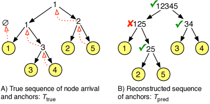
Figure 2B shows an example sequence of merges predicted by our reconstruction algorithms. Internal nodes in the tree are labeled with the concatenation of the labels of its two children indicating an inferred node/anchor relationship between the children.

Let $T_{\textrm{true}}$ be the anchor tree derived from the true growth process (Figure 2A) and let $T_{\textrm{pred}}$ be the reconstructed anchor tree (Figure 2B). We can assess the quality of the reconstruction by seeing what percentage of subtrees in $T_{\textrm{pred}}$ are found in $T_{\textrm{true}}$. This measure (called Anchor) is closely related to the Robinson-Foulds distance metric used to compare phylogenetic trees [6]. In the example of Figure 2, the similarity between the trees is $3/4=75\%$.

This validation measure is advantageous because it evaluates if the relationship between larger groups of nodes was correctly determined. In addition, it does not unduly penalize the mis-ordering of arrival times for nodes that are far apart in the network. It also does not depend on which node of the merged pair $(u,v)$ was deleted from the graph in the DMC model, because both choices lead to the same subtree in $T_{\textrm{pred}}$. On the other hand, the measure is in some ways stricter than counting correct node/anchor pairs. For example, in Figure 2 it would be incorrect to merge $1$ and $2$ in the first backward step because the extant nodes $1$ and $2$ are not the same as the past nodes $1$ and $2$.

4 Results

4.1 Model reversibility using the greedy likelihood algorithm

Figure 3: Accuracy of node arrival times and node anchors using the DMC model. The $x$ and $y$-axes show the DMC parameters ($q_{\textrm{mod}},q_{\textrm{con}}$) used to grow the synthetic network forward. Each parameter varies from $0.1$–$0.9$ in steps of $0.2$. The intensity of each cell in the heatmap represents the quality of the reconstruction validation measure (Anchor, Kendall, Footrule) under optimal reverse parameters. (A) and (B) show results under varying levels of noise. For many DMC-grown synthetic networks, accurate reconstruction is possible.

We first tested the algorithms in situations where the evolutionary history is completely known. This allows us to assess the performance of the greedy likelihood algorithm and to compare the reversibility of various network models. For each model (and choice of parameters), we grew $100$-node networks forward according to the model, and then supplied only the final network $G_{t=100}$ to our algorithm to reconstruct its history. We repeated this process $10$ times and averaged the results for each combination.

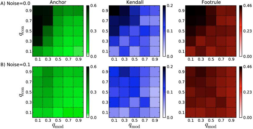
For the DMC model under realistic choices of $q_{\textrm{mod}}$ and $q_{\textrm{con}}$, almost $60\%$ of the node/anchor relationships inferred are correct if the optimal choice of $q_{\textrm{mod}}$ and $q_{\textrm{con}}$ parameters are used in the reconstruction process. Figure 3A plots the performance of the $3$ validation measures for $25$ combinations of $(q_{\textrm{mod}},q_{\textrm{con}})$ model parameters. Both the Spearman’s footrule and Kendall’s $\tau$ measures of arrival-time correlation reveal an ability to order nodes correctly significantly better than random. In general, it is difficult to predict all arrival times correctly because unrelated duplications could occur in successive steps in completely different parts of the graph. But still, a large agreement can be obtained from analysis of the final graph alone.

Reversibility varies drastically depending on the DMC model parameters used to grow the network forward. Naturally, increasing $q_{\textrm{mod}}$ induces more random changes in the network, which makes it more difficult to reverse the evolution. Conversely, as $q_{\textrm{con}}$ increases, the history generally becomes easier to reverse because more nodes are directly connected to the node from which they duplicated.

Figure 4: Accuracy of node arrival times and node anchors when reverse parameters are not known. Synthetic DMC-grown networks were constructed using $q_{\textrm{mod}}=0.1,q_{\textrm{con}}=0.9$ and reversed using all $25$ combinations of reversal parameters. The $x$ and $y$-axes show the difference between the reversal parameters ($rq_{\textrm{mod}}$ and $rq_{\textrm{con}}$, respectively) and the forward parameters ($0.1$ and $0.9$, respectively). The intensity of each cell in the heatmap represents the quality of the reconstruction validation measure (Anchor, Kendall, Footrule). Accurate histories can be inferred as long as reverse parameters (in particular, $rq_{\textrm{mod}}$) are in the rough range of the forward parameters.

Performance also depends on the match between the values of $q_{\textrm{mod}}$ and $q_{\textrm{con}}$ used to grow the network forward and those used to reverse the history (Figure 4). However, even if the forward parameters are not known exactly, it is feasible to reconstruct a meaningful history if the reversal parameters are chosen to be near the forward parameters. There is often a hard transition at $q_{\textrm{mod}}=0.5$ or $q_{\textrm{con}}=0.5$ when the bias towards having an edge and not having an edge tips to one side or the other. Though optimal performance can correspond to reversing a network with the same parameters used to grow the network, this need not be the case. For example, suppose $30$% of all nodes have edges to their anchors. This does not imply that setting $q_{\textrm{con}}=0.3$ will work best because the true pair sought will likely not be connected and hence even lower values of $q_{\textrm{con}}$ may lead to a more accurate reconstruction.

Figure 5: Accuracy of arrival times and node anchors using the forest fire model. (A–D) The $x$-axis shows the FF parameter ($p$) used to grow the synthetic network forward. The $y$-axis shows the quality of the $3$ reconstruction validation measures under optimal reverse parameters. All FF-based reconstructions are significantly better than random reconstructions, even when $30\%$ of true edges are replaced by random edges.

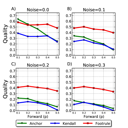
We performed the same synthetic-data experiments using the forest fire model for varying values of the parameter $p$, which controls the spread of the fire, ranging from $0.1$ to $0.5$. (Values of parameter $p>0.5$ resulted in mostly clique-like networks.) Figure 5A shows that between $25\%$ and $64\%$ of anchor relationships can be correctly identified, and that the estimated node arrival ordering resembles the true arrival order. As $p$ increases, performance of all measures tends to decrease. This is because as $p$ increases, the degree of each node increases, thus making it more difficult to pick out the correct anchor from among the set of neighbors.

Figure 6: Agreement with arrival times using the preferential attachment model. (A–D) The $x$-axis shows the PA parameter ($k$) used to grow the synthetic network forward. The $y$-axis show the quality of the $3$ reconstruction validation measures. Compared to the DMC and FF models, the PA model is easiest to reverse, even in the presence of substantial noise.

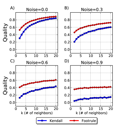
Finally, we grew $1000$-node networks using the linear preferential attachment model for various choices of parameter $k$, the number of neighbors to which a new node initially connects (Figure 6). Of the three models we consider, PA is the most easily reversible. As $k$ increases, there becomes more opportunity for older and newer nodes to differentiate themselves from one another, and hence the network becomes easier to reverse. Figure 6A shows that for the PA model we can achieve Kendall $\tau$ values of over $80$ percentage points higher than random when $k>15$. In the PA model, a new node does not choose an anchor node to copy links from so only the arrival-time validation measures are applicable.

4.2 Effect of deviation from the assumed model

To gauge robustness to deviations from the growth model, we repeated the experiments on synthetic data after randomly replacing some percentage of edges in the final graph with new edges. Under all models, reconstruction quality generally suffers from a noisy view of the present-day graph but meaningful histories can still be recovered.

DMC is the most sensitive to the addition of noise (Figure 3B), while PA is by far the most resilient to noise. Even when $90\%$ of the true edges are replaced with random edges, nearly turning the graph into a random graph, reversibility of PA is still better than random (Figure 6D). DMC can tolerate noise up to $30\%$ before returning essentially random reconstructions. The robustness of the forest fire model lies in between DMC and PA (Figure 5D).

Mis-identifying the model used to grow the network can also significantly reduce the quality of the inferred history. To verify this, we grew networks forward using DMC $(q_{\textrm{mod}}=0.1,q_{\textrm{con}}=0.9)$ and reversed it with the other models. The low $q_{\textrm{mod}}$ value implies that a node has many reasonable anchors. A reversal using the FF model cannot distinguish between these many reasonable anchors. In particular, FF performs approximately 10 times worse than DMC according to both the Spearman’s footrule and Kendall’s $\tau$ measures. Further, FF is only able to uncover an average of $4\%$ of correct node/anchor relationships compared to $55\%$ using DMC. PA also performs poorly in this case because nodes with late arrival times can duplicate from hubs and immediately become “hubby”. Hence, reversing DMC-grown networks involves more than removing low-degree nodes. As $q_{\textrm{mod}}$ increases, FF and PA each perform better at reversing DMC networks, but both still perform worse than DMC (e.g. at $q_{\textrm{mod}}=0.5$, FF and PA have average Kendall $\tau$ values of $9\%$ and $10\%$, respectively, compared to $15\%$ for DMC).

Random networks grown forward using PA are best reversed using PA as opposed to DMC or FF. At $k=10$, PA has a Kendall $\tau$ value of over $70\%$ compared to only $36\%$ for DMC and $20\%$ for FF. At higher values of $k$, this difference is even more pronounced. The reason DMC and FF perform so poorly is because, for each node, they seek a single anchor from which the observed links can be explained. With PA, however, a node can have neighbors that are far apart in the network.

4.3 Recovery of ancient protein interaction networks

Figure 7: Visualization [38] of the extant PPI network ($G_{t=2599}$) and an ancestral version ($G_{t=1300}$). The density, clustering coefficient (CC), average shortest path length (SPL), and average $k$-core number are shown for each network. The ancient network is considerably denser than the extant network.

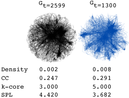
We obtained a high-confidence protein-protein interaction (PPI) network for the yeast S. cerevisiae from the IntAct database [20]. The network contains $2,599$ proteins (nodes) and $8,275$ physical interactions between them. We applied the reversal algorithm for $2,599$ steps to estimate a complete history of the growth of the network. Figure 7 shows the original network ($G_{t=2599}$) and an inferred ancestral network with $1300$ nodes ($G_{t=1300}$).

Because PPI networks from the past are unavailable, we do not directly have true node arrival times to which we can compare. Instead, we estimate protein arrival times using sequence-based homology under the assumption that proteins that have emerged after yeast diverged from other species will have fewer orthologs in these distantly related organisms [29]. In particular, we obtained data for the occurrence of orthologs of yeast proteins in 6 eukaryotes (A. thaliana, C. elegans, D. melanogaster, H. sapiens, S. pombe, and E. cuniculi) from the Clusters of Orthologous Genes database [41]. The number of species for which an ortholog was present was used as a proxy for the arrival time: proteins with orthologs in $6$ of the eukaryotes are likely to be older than proteins with orthologs in $5$, and so on.

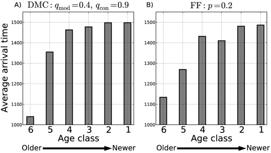
Reversing the network using the DMC model produced an estimated node arrival order in greater concordance with the orthology-based estimates of protein age than either the FF or PA models. Figure 8 shows the average reconstructed arrival time for proteins in each of the $6$ age classes for the DMC and FF models (the results for PA were similar to FF). The results shown are the best for each model over the tested parameter space and thus represent the limit of performance for each of the models using the proposed algorithm. The DMC model (Figure 8A) correctly determines the relative ordering of all the age classes ($P$-value $<0.01$ after Bonferroni correcting for optimal parameter usage). While the FF model does reconstruct the ordering of some of the age classes, it never produces the exact ordering for any choice of parameters (consistently swapping classes $3$ and $4$; Figure 8B). This provides additional evidence [31] that a DMC-like model is a better fit for PPI networks than models such as FF and PA inspired by social networks.

Figure 8: Predicting protein age groups by reversing the DMC and FF models on a real PPI network for S. cerevisiae. The $x$-axis shows the 6 age classes for proteins. The $y$-axis shows the average arrival time for proteins in the class. The DMC model correctly orders all classes, whereas the FF model swaps classes 3 and 4.

4.4 Estimation of parameters governing network growth

The parameters that produced the history that best matched the sequence-based estimates of protein ages provide hints about the relative importance of various processes in network growth. For DMC, the optimal parameters were $q_{\textrm{mod}}=0.4$ and $q_{\textrm{con}}=0.9$. We can use these as estimates of the probability that an interaction is modified following a gene duplication ($\approx 50$%) and the probability that two duplicated genes interact (high, as also found elsewhere [18, 36, 34]).

Interestingly, the optimal FF and DMC parameters create models that have many similarities. Optimal performance was obtained for the FF model with parameter $p=0.2$, which implies that both the anchor and the arriving node will have similar neighborhoods because the simulated fire likely does not spread beyond the immediate neighbors of the anchor. The property of similar neighborhoods is also implied by duplication step of DMC coupled with the moderate value of $q_{\textrm{mod}}=0.4$. Further, in the FF model the arriving node is always linked to its anchor, and the high value of $q_{\textrm{con}}=0.9$ causes this to frequently happen in the DMC model as well. Thus, based on their agreement with sequence-based estimates of protein arrival times, two independent and very different base models both suggest that proteins should very frequently interact with the protein from which they duplicated, and that the new node should primarily interact with neighbors of their anchors.

4.5 Protein complexes and evolution by duplication

We can test correctness of the anchors identified by DMC and FF using protein annotations. A protein and its duplicate are often involved in similar protein complexes in the cell [37, 36]. We expect then that the node/anchor pairs identified ought to correspond to proteins that are co-complexed. Because it is difficult to model the gain and loss of functional properties of ancient proteins, we only tested this hypothesis among pairs of extant proteins.

Using the MIPS complex catalog [12], which contained annotations for $994$ of the proteins in the network, $79\%$ of the testable node/anchor pairs predicted using the DMC model shared an annotation. This is much higher than the baseline frequency: only $55\%$ of edges in the extant network connect nodes that share an annotation. Under the FF model, $68\%$ of node/anchor pairs share a MIPS annotation. So, while the FF model under this validation measure again is performing much better than expected by random chance, it does not perform as well as DMC. The high quality of the DMC-based node/anchor pairs also supports the idea that a good definition of a functional module in a PPI network is one which groups proteins with similar neighbors together (rather than one based strictly on density) [34].

Figure 9: (A) The distribution of duplication rates for extant proteins in the PPI network. The $x$-axis of the histogram is the number of duplications, measured as the distance from the root of the phylogeny to the extant protein. The $y$-axis is the percentage of proteins lying in the tree depth bin. (B) The relationship between duplication and number of interaction partners. The $x$-axis shows the average tree depth for proteins with the given number of interaction partners ($y$-axis) in $G_{t=2599}$.

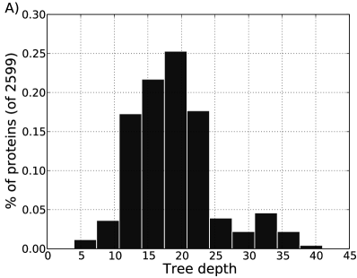
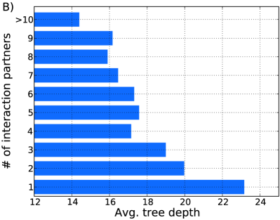
The phylogeny of node/anchor relationships can also help characterize how duplication has guided the evolution of the yeast proteome. We estimate the number of times each extant protein was involved in a duplication (that becomes fixed in the population) by computing the depth of the protein in the inferred node/anchor tree. Figure 9A shows that most proteins are involved in a similar number of duplications (mean = 19), with fewer proteins involved in many more or many less. Proteins involved in more duplications typically have fewer interaction partners (Figure 9B). Using network histories alone, this confirms previous sequence-based findings that the evolutionary rate of proteins is inversely proportional to its number of binding partners [8, 30].

The arrival times of proteins can also tell us how different components of protein complexes might have evolved. For every protein belonging to exactly one MIPS complex, we computed its coreness, defined as the percentage of its annotated neighbors that belong to the same complex. A large coreness value indicates that the protein plays a central role in the complex; a small value suggests a peripheral role [9]. Amongst the $763$ protein tested, there was a significant correlation between older proteins and larger coreness values ($R=0.36$, $P$-value $<0.01$), a trend that Kim and Marcotte, [21] also independently reported by studying the evolution of protein structure using a different measure of coreness.

4.6 Recovery of past social networks

To contrast the evolution of biological networks with social networks, we applied our algorithms to part of the Last.fm music social network. Edges in this network link users (nodes) that are friends. We sampled a region of the network by performing a breadth-first crawl starting from a random user ‘rj’. We recorded the date and time of registration for each node visited, which corresponds to its arrival time into the network. The resulting network consisted of the subgraph induced by the first $2,957$ nodes visited ($9,659$ edges). Because only a subgraph of the complete network was visited, some nodes have neighbors that are outside the induced subgraph. This missing data makes the reconstruction problem even more difficult.

Figure 10: Predicting node arrival times for users in the Last.fm social network. The PA model appears most applicable to reversing the network.

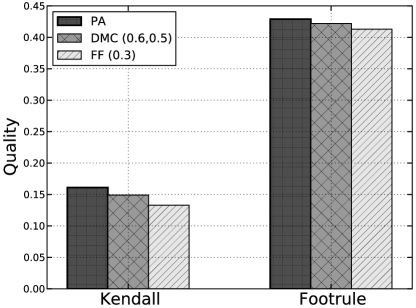
Figure 10 shows the performance of the models (using the best parameters) for the node-arrival measures. The best performing model (preferential attachment) for the Last.fm network was the worse performing model for the PPI network. Further, the optimal FF value of $p$ for the Last.fm network was larger ($0.3$) than for the PPI network ($0.2$). This fits well with the notion that new users in social networks often form links to a varied set of existing users that might be far apart in the network [26].

An advantage of FF and DMC over PA is that the former return node anchors. To validate these predicted relationships, we make the observation that node/anchor pairs are likely to share similar taste in music. As a null baseline, we computed the percentage of edges in the given network $G_{t=2957}$ that connect users who share a top-5 favorite artist. The pairs returned by FF are significantly more likely ($13.8\%$) to share a top-5 favorite artist over DMC $(10.3\%)$ and the baseline $(10.8\%)$. Most users act as anchors to $\leq 1$ new member, however, there were $9$ users who (putatively) each brought $\geq 30$ new members into the network. Such popular anchors can be thought of as members who are responsible for the network’s organic growth.

5 Discussion

We presented a novel framework for uncovering precursor versions of a network given only a growth model by which the network putatively evolved. Our approach works backwards from a given network and is therefore network specific (not model generic) and can retain individual node labels.

Using the proposed algorithms, we estimated protein ages from the topology of a PPI alone that matched sequence-based estimates well. Further, we correlated node/anchor pairs with co-complexed proteins and characterized the distribution of duplications on a per-protein basis. We also found that older proteins tend to play a more central role in protein complexes than newer, peripheral proteins. Given the noisy and incomplete status of the available PPI data and the simple network growth models, it is surprising that such high agreement with known biology can be obtained.

We also used the accuracy of history reconstruction as an optimization criterion for choosing model parameters. We determined, via both the DMC and FF models, that duplicated proteins are likely to interact and share many interaction partners. The ability to match the inferred history under a given model to properties of the true history provides an alternative way to validate models that goes beyond comparing only statistics of the final extant network.

A heuristic approach that orders node arrival times based on their static degree in the extant network performs similarly to PA (poor performance on DMC-grown synthetic networks and the PPI network; better performance for PA-grown synthetic networks and the Last.fm network). PA is derived from the assumption that degree distribution is correlated with age, hence the similarity is to be expected. The drawback with such a heuristic is that it does not provide a likelihood estimate for a history, in contrast to our more principled approach.

A natural extension to this work is to evaluate how the greedy likelihood approach performs on other models, such as those that explicitly incorporate an estimate of a node’s age [31, 21] or those in which nodes can add edges at variable times [23]. Automated selection of reverse model parameters and computation of model-based priors to use in the likelihood procedure may make the reconstructions more accurate and more practical. However, even with the standard models investigated here, our results show that present-day networks are strongly linked to their past, and that this past can be effectively excavated.

References

- Ahmed and Xing, [2009] Ahmed, A. and Xing, E. P. (2009). Recovering time-varying networks of dependencies in social and biological studies. Proc. Natl. Acad. Sci. USA, 106:11878–11883.
- Bar-Ilan et al., [2006] Bar-Ilan, J., Mat-Hassan, M., and Levene, M. (2006). Methods for comparing rankings of search engine results. Comput. Netw., 50(10):1448–1463.
- Barab\a’asi and Albert, [1999] Barab\a’asi, A. L. and Albert, R. (1999). Emergence of scaling in random networks. Science, 286(5439):509–512.
- Bezáková et al., [2006] Bezáková, I., Kalai, A., and Santhanam, R. (2006). Graph model selection using maximum likelihood. In Proc. 23rd Intl. Conf. on Maching Learning, pages 105–112.
- Dutkowski and Tiuryn, [2007] Dutkowski, J. and Tiuryn, J. (2007). Identification of functional modules from conserved ancestral protein-protein interactions. Bioinformatics, 23(13):i149–i158.
- Felsenstein, [2003] Felsenstein, J. (2003). Inferring Phylogenies. Sinauer Associates, 2nd edition.
- Flannick et al., [2006] Flannick, J., Novak, A., Srinivasan, B. S., McAdams, H. H., and Batzoglou, S. (2006). Graemlin: general and robust alignment of multiple large interaction networks. Genome Res., 16(9):1169–1181.
- Fraser et al., [2002] Fraser, H. B., Hirsh, A. E., Steinmetz, L. M., Scharfe, C., and Feldman, M. W. (2002). Evolutionary rate in the protein interaction network. Science, 296(5568):750–752.
- Gavin et al., [2006] Gavin, A.-C., Aloy, P., Grandi, P., Krause, R., Boesche, M., Marzioch, M., Rau, C., Jensen, L. J., Bastuck, S., Dümpelfeld, B., Edelmann, A., Heurtier, M.-A., Hoffman, V., Hoefert, C., Klein, K., Hudak, M., Michon, A.-M., Schelder, M., Schirle, M., Remor, M., Rudi, T., Hooper, S., Bauer, A., Bouwmeester, T., Casari, G., Drewes, G., Neubauer, G., Rick, J. M., Kuster, B., Bork, P., Russell, R. B., and Superti-Furga, G. (2006). Proteome survey reveals modularity of the yeast cell machinery. Nature, 440:631–636.
- Gibson and Goldberg, [2009] Gibson, T. A. and Goldberg, D. S. (2009). Reverse engineering the evolution of protein interaction networks. Pac. Symp. Biocomput., pages 190–202.
- Golbeck, [2007] Golbeck, J. (2007). The dynamics of web-based social networks: Membership, relationships, and change. First Monday, 12(11).
- Guldener et al., [2005] Guldener, U. et al. (2005). CYGD: the comprehensive yeast genome database. Nucleic Acids Res., 33(Suppl. 1):D364+.
- Guo et al., [2007] Guo, F., Hanneke, S., Fu, W., and Xing, E. (2007). Recovering temporally rewiring networks: A model-based approach. In Proc. 24th Intl. Conf. on Machine Learning, pages 321–328.
- Hanneke and Xing, [2007] Hanneke, S. and Xing, E. (2007). Discrete temporal models of social networks. In Proc. 23rd Intl. Conf. on Maching Learning, Workshop on Statistical Network Analysis, pages 115–125.
- Hopcroft et al., [2004] Hopcroft, J., Khan, O., Kulis, B., and Selman, B. (2004). Tracking evolving communities in large linked networks. Proc. Natl. Acad. Sci. USA, 101(Suppl. 1):5249–5253.
- Hormozdiari et al., [2007] Hormozdiari, F., Berenbrink, P., Prz̆ulj, N., and Sahinalp, S. C. (2007). Not all scale-free networks are born equal: The role of the seed graph in PPI network evolution. PLoS Comput. Biol., 3(7):e118.
- [17] Ispolatov, I., Krapivsky, P. L., and Yuryev, A. (2005a). Duplication-divergence model of protein interaction network. Phys Rev. E, 71(6 Pt 1):061911.
- [18] Ispolatov, I., Yuryev, A., Mazo, I., and Maslov, S. (2005b). Binding properties and evolution of homodimers in protein-protein interaction networks. Nucleic Acids Res., 33(11):3629–3635.
- Kelley et al., [2003] Kelley, B. P., Sharan, R., Karp, R. M., Sittler, T., Root, D. E., Stockwell, B. R., and Ideker, T. (2003). Conserved pathways within bacteria and yeast as revealed by global protein network alignment. Proc. Natl. Acad. Sci. USA, 100(20):11394–11399.
- Kerrien et al., [2007] Kerrien, S. et al. (2007). Intact–open source resource for molecular interaction data. Nucleic Acids Res., 35(Database issue).
- Kim and Marcotte, [2008] Kim, W. K. and Marcotte, E. M. (2008). Age-dependent evolution of the yeast protein interaction network suggests a limited role of gene duplication and divergence. PLoS Comput. Biol., 4(11):e1000232.
- Kumar et al., [2006] Kumar, R., Novak, J., and Tomkins, A. (2006). Structure and evolution of online social networks. In Proc. 12th Intl. Conf. on Knowledge Discovery and Data mining, pages 611–617.
- Leskovec et al., [2008] Leskovec, J., Backstrom, L., Kumar, R., and Tomkins, A. (2008). Microscopic evolution of social networks. In Proc. 14th Intl. Conf. on Knowledge Discovery and Data mining, pages 462–470.
- Leskovec et al., [2010] Leskovec, J., Chakrabarti, D., Kleinberg, J., Faloutsos, C., and Ghahramani, Z. (2010). Kronecker graphs: An approach to modeling networks. J. Mach. Learn. Res., 11:985–1042.
- Leskovec and Faloutsos, [2007] Leskovec, J. and Faloutsos, C. (2007). Scalable modeling of real graphs using Kronecker multiplication. In Proc. 24th Intl. Conf. on Machine Learning, pages 497–504.
- Leskovec et al., [2005] Leskovec, J., Kleinberg, J., and Faloutsos, C. (2005). Graphs over time: densification laws, shrinking diameters and possible explanations. In Proc. 11th Intl. Conf. on Knowledge Discovery and Data mining, pages 177–187.
- Leskovec et al., [2007] Leskovec, J., McGlohon, M., Faloutsos, C., Glance, N., and Hurst, M. (2007). Cascading behavior in large blog graphs: Patterns and a model. In Proc. 7th SIAM Intl. Conf. on Data Mining.
- Levy and Pereira-Leal, [2008] Levy, E. D. and Pereira-Leal, J. B. (2008). Evolution and dynamics of protein interactions and networks. Curr. Opin. Struct. Biol., 18(3):349–357.
- Li et al., [2004] Li, S. et al. (2004). A map of the interactome network of the metazoan C. elegans. Science, 303(5657):540–543.
- Makino et al., [2006] Makino, T., Suzuki, Y., and Gojobori, T. (2006). Differential evolutionary rates of duplicated genes in protein interaction network. Gene, 385:57–63.
- Middendorf et al., [2005] Middendorf, M., Ziv, E., and Wiggins, C. H. (2005). Inferring network mechanisms: the Drosophila melanogaster protein interaction network. Proc. Natl. Acad. Sci. USA, 102(9):3192–3197.
- Milo et al., [2002] Milo, R., Shen-Orr, S., Itzkovitz, S., Kashtan, N., Chklovskii, D., and Alon, U. (2002). Network motifs: Simple building blocks of complex networks. Science, 298(5594):824–827.
- Mithani et al., [2009] Mithani, A., Preston, G., and Hein, J. (2009). A stochastic model for the evolution of metabolic networks with neighbor dependence. Bioinformatics, 25(12):1528–1535.
- Navlakha et al., [2009] Navlakha, S., Schatz, M. C., and Kingsford, C. (2009). Revealing biological modules via graph summarization. J. Comp. Biol., 16(2):253–264.
- Palla et al., [2007] Palla, G., Barab\a’asi, A. L., and Vicsek, T. (2007). Quantifying social group evolution. Nature, 446(7136):664–667.
- Pereira-Leal et al., [2007] Pereira-Leal, J. B., Levy, E. D., Kamp, C., and Teichmann, S. A. (2007). Evolution of protein complexes by duplication of homomeric interactions. Genome Biol., 8(4):R51.
- Pereira-Leal et al., [2006] Pereira-Leal, J. B., Levy, E. D., and Teichmann, S. A. (2006). The origins and evolution of functional modules: lessons from protein complexes. Philos. Trans. R Soc. Lond. B Biol. Sci., 361(1467):507–517.
- Shannon et al., [2003] Shannon, P., Markiel, A., Ozier, O., Baliga, N. S., Wang, J. T., Ramage, D., Amin, N., Schwikowski, B., and Ideker, T. (2003). Cytoscape: a software environment for integrated models of biomolecular interaction networks. Genome Res., 13(11):2498–2504.
- Singh et al., [2007] Singh, R., Xu, J., and Berger, B. (2007). Pairwise global alignment of protein interaction networks by matching neighborhood topology. In Proc. 11th Intl. Conf. on Research in Computational Molecular Biology (RECOMB), pages 16–31.
- Tantipathananandh and Berger-Wolf, [2009] Tantipathananandh, C. and Berger-Wolf, T. (2009). Constant-factor approximation algorithms for identifying dynamic communities. In Proc. 15th Intl. Conf. on Knowledge Discovery and Data mining, pages 827–836.
- Tatusov et al., [2003] Tatusov, R. et al. (2003). The COG database: an updated version includes eukaryotes. BMC Bioinformatics, 4:41.
- Vazquez et al., [2003] Vazquez, A., Flammini, A., Maritan, A., and Vespignani, A. (2003). Modeling of protein interaction networks. Complexus, 1(1):38–44.
- Wagner, [2003] Wagner, A. (2003). How the global structure of protein interaction networks evolves. Proc. Biol. Sci., 270(1514):457–466.
- Watts and Strogatz, [1998] Watts, D. J. and Strogatz, S. H. (1998). Collective dynamics of ‘small-world’ networks. Nature, 393(6684):440–442.
- Wiuf et al., [2006] Wiuf, C., Brameier, M., Hagberg, O., and Stumpf, M. P. (2006). A likelihood approach to analysis of network data. Proc. Natl. Acad. Sci. USA, 103(20).