Data analysis recipes:
Fitting a model to data***The notes begin on page Notes, including the
license1 and
the acknowledgements2.
David W. Hogg
Center for Cosmology and Particle Physics, Department of Physics, New York University
Max-Planck-Institut für Astronomie, Heidelberg
Jo Bovy
Center for Cosmology and Particle Physics, Department of Physics, New York University
Dustin Lang
Department of Computer Science, University of Toronto
Princeton University Observatory
Abstract
We go through the many considerations involved in fitting a model to data, using as an example the fit of a straight line to a set of points in a two-dimensional plane. Standard weighted least-squares fitting is only appropriate when there is a dimension along which the data points have negligible uncertainties, and another along which all the uncertainties can be described by Gaussians of known variance; these conditions are rarely met in practice. We consider cases of general, heterogeneous, and arbitrarily covariant two-dimensional uncertainties, and situations in which there are bad data (large outliers), unknown uncertainties, and unknown but expected intrinsic scatter in the linear relationship being fit. Above all we emphasize the importance of having a “generative model” for the data, even an approximate one. Once there is a generative model, the subsequent fitting is non-arbitrary because the model permits direct computation of the likelihood of the parameters or the posterior probability distribution. Construction of a posterior probability distribution is indispensible if there are “nuisance parameters” to marginalize away.
It is conventional to begin any scientific document with an introduction that explains why the subject matter is important. Let us break with tradition and observe that in almost all cases in which scientists fit a straight line to their data, they are doing something that is simultaneously wrong and unnecessary. It is wrong because circumstances in which a set of two dimensional measurements—outputs from an observation, experiment, or calculation—are truly drawn from a narrow, linear relationship is exceedingly rare. Indeed, almost any transformation of coordinates renders a truly linear relationship non-linear. Furthermore, even if a relationship looks linear, unless there is a confidently held theoretical reason to believe that the data are generated from a linear relationship, it probably isn’t linear in detail; in these cases fitting with a linear model can introduce substantial systematic error, or generate apparent inconsistencies among experiments that are intrinsically consistent.
Even if the investigator doesn’t care that the fit is wrong, it is likely to be unnecessary. Why? Because it is rare that, given a complicated observation, experiment, or calculation, the important result of that work to be communicated forward in the literature and seminars is the slope and intercept of a best-fit line! Usually the full distribution of data is much more rich, informative, and important than any simple metrics made by fitting an overly simple model.
That said, it must be admitted that one of the most effective ways to communicate scientific results is with catchy punchlines and compact, approximate representations, even when those are unjustified and unnecessary. It can also sometimes be useful to fit a simple model to predict new data, given existing data, even in the absence of a physical justification for the fit.3 For these reasons—and the reason that in rare cases the fit is justifiable and essential—the problem of fitting a line to data comes up very frequently in the life of a scientist.
It is a miracle with which we hope everyone reading this is familiar that if you have a set of two-dimensional points that depart from a perfect, narrow, straight line only by the addition of Gaussian-distributed noise of known amplitudes in the direction only, then the maximum-likelihood or best-fit line for the points has a slope and intercept that can be obtained justifiably by a perfectly linear matrix-algebra operation known as “weighted linear least-square fitting”. This miracle deserves contemplation.
Once any of the input assumptions is violated (and note there are many input assumptions), all bets are off, and there are no consensus methods used by scientists across disciplines. Indeed, there is a large literature that implies that the violation of the assumptions opens up to the investigator a wide range of possible options with little but aesthetics to distinguish them! Most of these methods of “linear regression” (a term we avoid) performed in science are either unjustifiable or else unjustified in almost all situations in which they are used.4 Perhaps because of this plethora of options, or perhaps because there is no agreed-upon bible or cookbook to turn to, or perhaps because most investigators would rather make some stuff up that works “good enough” under deadline, or perhaps because many realize, deep down, that much fitting is really unnecessary anyway, there are some egregious procedures and associated errors and absurdities in the literature.5 When an investigator cites, relies upon, or transmits a best-fit slope or intercept reported in the literature, he or she may be propagating more noise than signal.
It is one of the objectives of this document to promote an understanding that if the data can be modeled statistically there is little arbitrariness. It is another objective to promote consensus; when the choice of method is not arbitrary, consensus will emerge automatically. We present below simple, straightforward, comprehensible, and—above all—justifiable methods for fitting a straight line to data with general, non-trivial, and uncertain properties.
This document is part polemic (though we have tried to keep most of the polemic in the notes), part attempt at establishing standards, and part crib sheet for our own future re-use. We apologize in advance for some astrophysics bias and failure to review basic ideas of linear algebra, function optimization, and practical statistics. Very good reviews of the latter exist in abundance.6 We also apologize for not reviewing the literature; this is a cheat-sheet not a survey. Our focus is on the specific problems of linear fitting that we so often face; the general ideas appear in the context of these concrete and relatively realistic example problems. The reader is encouraged to do the Exercises; many of these ask you to produce plots which can be compared with the Figures.
Section 1 Standard practice
You have a set of points , with known Gaussian uncertainties in the direction, and no uncertainty at all (that is, perfect knowledge) in the direction. You want to find the function of the form
| (1) |
where is the slope and is the intercept, that best fits the points. What is meant by the term “best fit” is, of course, very important; we are making a choice here to which we will return. For now, we describe standard practice:
Construct the matrices
| (6) | ||||
| (11) | ||||
| (16) |
where one might call a “vector”, and the covariance matrix could be generalized to the non-diagonal case in which there are covariances among the uncertainties of the different points. The best-fit values for the parameters and are just the components of a column vector found by
| (17) |
This is actually the simplest thing that can be written down that is linear, obeys matrix multiplication rules, and has the right relative sensitivity to data of different statistical significance. It is not just the simplest thing; it is the correct thing, when the assumptions hold.7 It can be justified in one of several ways; the linear algebra justification starts by noting that you want to solve the equation
| (18) |
but you can’t because that equation is over-constrained. So you weight everything with the inverse of the covariance matrix (as you would if you were doing, say, a weighted average), and then left-multiply everything by to reduce the dimensionality, and then equation (17) is the solution of that reduced-dimensionality equation.
This procedure is not arbitrary; it minimizes an objective function8 (“chi-squared”), which is the total squared error, scaled by the uncertainties, or
| (19) |
that is, equation (17) yields the values for and that minimize . Conceptually, is like a metric distance in the data space.9 This, of course, is only one possible meaning of the phrase “best fit”; that issue is addressed more below.
When the uncertainties are Gaussian and their variances are correctly estimated, the matrix that appears in equation (17) is just the covariance matrix (Gaussian uncertainty—uncertainty not error10—variances on the diagonal, covariances off the diagonal) for the parameters in . We will have more to say about this in Section 4.
| ID | ||||||
|---|---|---|---|---|---|---|
| 1 | 201 | 592 | 61 | 9 | -0. | 84 |
| 2 | 244 | 401 | 25 | 4 | 0. | 31 |
| 3 | 47 | 583 | 38 | 11 | 0. | 64 |
| 4 | 287 | 402 | 15 | 7 | -0. | 27 |
| 5 | 203 | 495 | 21 | 5 | -0. | 33 |
| 6 | 58 | 173 | 15 | 9 | 0. | 67 |
| 7 | 210 | 479 | 27 | 4 | -0. | 02 |
| 8 | 202 | 504 | 14 | 4 | -0. | 05 |
| 9 | 198 | 510 | 30 | 11 | -0. | 84 |
| 10 | 158 | 416 | 16 | 7 | -0. | 69 |
| 11 | 165 | 393 | 14 | 5 | 0. | 30 |
| 12 | 201 | 442 | 25 | 5 | -0. | 46 |
| 13 | 157 | 317 | 52 | 5 | -0. | 03 |
| 14 | 131 | 311 | 16 | 6 | 0. | 50 |
| 15 | 166 | 400 | 34 | 6 | 0. | 73 |
| 16 | 160 | 337 | 31 | 5 | -0. | 52 |
| 17 | 186 | 423 | 42 | 9 | 0. | 90 |
| 18 | 125 | 334 | 26 | 8 | 0. | 40 |
| 19 | 218 | 533 | 16 | 6 | -0. | 78 |
| 20 | 146 | 344 | 22 | 5 | -0. | 56 |
Note. — The full uncertainty covariance matrix for each data point is given by
.
Exercise 0:
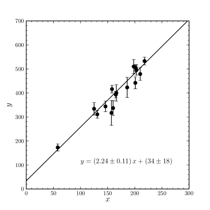
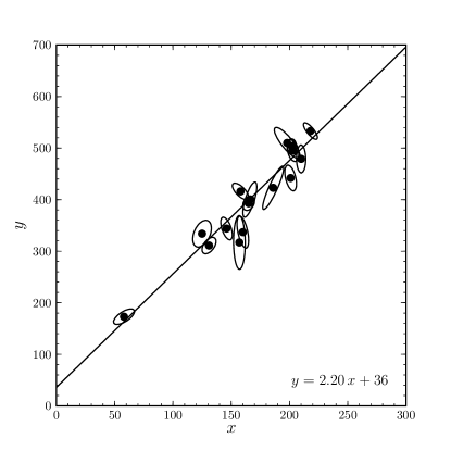
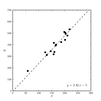
Using the standard linear algebra method of this Section, fit the straight line to the , , and values for data points 5 through 20 in Table LABEL:table:data_allerr on page LABEL:table:data_allerr. That is, ignore the first four data points, and also ignore the columns for and . Make a plot showing the points, their uncertainties, and the best-fit line. Your plot should end up looking like Figure 1. What is the standard uncertainty variance on the slope of the line?
Exercise 1:
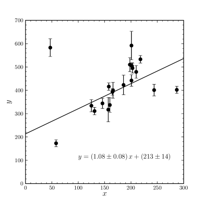
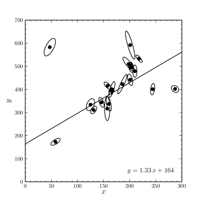
Repeat Exercise 1 but for all the data points in Table LABEL:table:data_allerr on page LABEL:table:data_allerr. Your plot should end up looking like Figure 2. What is the standard uncertainty variance on the slope of the line? Is there anything you don’t like about the result? Is there anything different about the new points you have included beyond those used in Exercise 1?
Exercise 2:
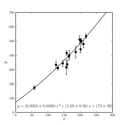
Generalize the method of this Section to fit a general quadratic (second order) relationship. Add another column to matrix containing the values , and another element to vector (call it ). Then re-do Exercise 1 but fitting for and plotting the best quadratic relationship
| (20) |
Your plot should end up looking like Figure 3.
Section 2 The objective function
A scientist’s justification of equation (17) cannot appeal purely to abstract ideas of linear algebra, but must originate from the scientific question at hand. Here and in what follows, we will advocate that the only reliable procedure is to use all one’s knowledge about the problem to construct a (preferably) justified, (necessarily) scalar (or, at a minimum, one-dimensional), objective function that represents monotonically the quality of the fit.11 In this framework, fitting anything to anything involves a scientific question about the objective function representing “goodness of fit” and then a separate and subsequent engineering question about how to find the optimum and, possibly, the posterior probability distribution function around that optimum.12 Note that in the previous Section we did not proceed according to these rules; indeed the procedure was introduced prior to the objective function, and the objective function was not justified.
In principle, there are many choices for objective function. But the only procedure that is truly justified—in the sense that it leads to interpretable probabilistic inference, is to make a generative model for the data. A generative model is a parameterized, quantitative description of a statistical procedure that could reasonably have generated the data set you have. In the case of the straight line fit in the presence of known, Gaussian uncertainties in one dimension, one can create this generative model as follows: Imagine that the data really do come from a line of the form , and that the only reason that any data point deviates from this perfect, narrow, straight line is that to each of the true values a small -direction offset has been added, where that offset was drawn from a Gaussian distribution of zero mean and known variance . In this model, given an independent position , an uncertainty , a slope , and an intercept , the frequency distribution for is
| (21) |
where this gives the expected frequency (in a hypothetical set of repeated experiments13) of getting a value in the infinitesimal range per unit .
The generative model provides us with a natural, justified, scalar objective: We seek the line (parameters and ) that maximize the probability of the observed data given the model or (in standard parlance) the likelihood of the parameters.14 In our generative model the data points are independently drawn (implicitly), so the likelihood is the product of conditional probabilities
| (22) |
Taking the logarithm,
| (23) | |||||
where is some constant. This shows that likelihood maximization is identical to minimization and we have justified, scientifically, the procedure of the previous Section.
The Bayesian generalization of this is to say that
| (24) |
where and are the model parameters, is a short-hand for all the data , is a short-hand for all the prior knowledge of the and the and everything else about the problem15, is the posterior probability distribution for the parameters given the data and the prior knowledge, is the likelihood just computed in equation (22) (which is a frequency distribution for the data), is the prior probability distribution for the parameters that represents all knowledge except the data , and the denominator can—for our purposes—be thought of as a normalization constant, obtained by marginalizing the numerator over all parameters. Unless the prior has a lot of variation in the region of interest, the posterior distribution function here is going to look very similar to the likelihood function in equation (22) above. That is, with an uninformative prior, the straight line that maximizes the likelihood will come extremely close to maximizing the posterior probability distribution function; we will return to this later.
We have succeeded in justifying the standard method as optimizing a justified, scalar objective function; the likelihood of a generative model for the data. It is just the great good luck of Gaussian distributions that the objective can be written as a quadratic function of the data. This makes the optimum a linear function of the data, and therefore trivial to obtain. This is a miracle.16
Exercise 3:
Imagine a set of measurements , with uncertainty variances , all of the same (unknown) quantity . Assuming the generative model that each differs from by a Gaussian-distributed offset, taken from a Gaussian with zero mean and variance , write down an expression for the log likelihood for the data given the model parameter . Take a derivative and show that the maximum likelihood value for is the usual weighted mean.
Exercise 4:
Section 3 Pruning outliers
The standard linear fitting method is very sensitive to outliers, that is, points that are substantially farther from the linear relation than expected—or not on the relation at all—because of unmodeled experimental uncertainty or unmodeled but rare sources of noise (or because the model has a restricted scope and doesn’t apply to all the data). There are two general approaches to mitigating this sensitivity, which are not necessarily different. The first is to find ways to objectively remove, reject, or become insensitive to “bad” points; this is the subject of this Section. The second is to better model your data-point uncertainties, permitting larger deviations than the Gaussian noise estimates; this is the subject of Section 5. Both of these are strongly preferable to sorting through the data and rejecting points by hand, for reasons of subjectivity and irreproducibility that we need not state. They are also preferable to the standard (in astrophysics anyway) procedure known as “sigma clipping”, which is a procedure and not the outcome of justifiable modeling.17
If we want to explicitly and objectively reject bad data points, we must add to the problem a set of binary integers , one per data point, each of which is unity if the th data point is good, and zero if the th data point is bad.18 In addition, to construct an objective function, one needs a parameter , the prior probability that any individual data point is bad, and parameters , the mean and variance of the distribution of bad points (in ). We need these latter parameters because, as we have emphasized above, our inference comes from evaluating a probabilistic generative model for the data, and that model must generate the bad points as well as the good points!
All these extra parameters may seem like crazy baggage, but their values can be inferred and marginalized out so in the end, we will be left with an inference just of the line parameters . In general, there is no reason to be concerned just because you have more parameters than data.19 However, the marginalization will require that we have a measure on our parameters (integrals require measures) and that measure is provided by a prior. That is, the marginalization will require, technically, that we become Bayesian; more on this below.
In this case, the likelihood is
| (25) | |||||
where and are the generative models for the foreground (good, or straight-line) and background (bad, or outlier) points. Because we are permitting data rejection, there is an important prior probability on the that penalizes each rejection:
| (26) |
that is, the binomial probability of the particular sequence . The priors on the other parameters should either be set according to an analysis of your prior knowledge or else be uninformative (as in flat in in the range , flat in in some reasonable range, and flat in the logarithm of in some reasonable range). If your data are good, it won’t matter whether you choose uninformative priors or priors that really represent your prior knowledge; in the end good data dominate either.
We have made a somewhat restrictive assumption that all data points are equally likely a priori to be bad, but you rarely know enough about the badness of your data to assume anything better.20 The fact that the prior probabilities are all set equal, however, does not mean that the posterior probabilities that individual points are bad will be at all similar. Indeed, this model permits an objective ranking (and hence public embarassment) of different contributions to any data set.21
We have used in this likelihood formulation a Gaussian model for the bad points; is that permitted? Well, we don’t know much about the bad points (that is one of the things that makes them bad), so this Gaussian model must be wrong in detail. But the power of this and the methods to follow comes not from making an accurate model of the outliers, it comes simply from modeling them. If you have an accurate or substantiated model for your bad data, use it by all means. If you don’t, because the Gaussian is the maximum-entropy distribution described by a mean and a variance, it is—in some sense—the least restrictive assumption, given that we have allowed that mean and variance to vary in the fitting (and, indeed, we will marginalize over both in the end).
The posterior probability distribution function, in general, is the likelihood times the prior, properly normalized. In this case, the posterior we (tend to) care about is that for the line parameters . This is the full posterior probability distribution marginalized over the bad-data parameters . Defining for brevity, the full posterior is
| (27) |
where the denominator can—for our purposes here—be thought of as a normalization integral that makes the posterior distribution function integrate to unity. The marginalization looks like
| (28) |
where by the integral over we really mean a sum over all of the possible settings of the , and the integrals over the other parameters are over their entire prior support. Effectively, then, this marginalization involves evaluating different likelihoods and marginalizing each one of them over ! Of course, because very few points are true candidates for rejection, there are many ways to “trim the tree” and do this more quickly, but thought is not necessary: Marginalization is in fact analytic.
Marginalization of this—what we will call “exponential”—model leaves a much more tractable—what we will call “mixture”—model. Imagine marginalizing over an individual . After this marginalization, the th point can be thought of as being drawn from a mixture (sum with amplitudes that sum to unity) of the straight-line and outlier distributions. That is, the generative model for the data integrates (or sums, really) to
| (29) | |||||
where and are the generative models for the foreground and background points, is the probability that a data point is bad (or, more properly, the amplitude of the bad-data distribution function in the mixture), and are parameters of the bad-data distribution.
Marginalization of the posterior probability distribution function generated by the product of the mixture likelihood in equation (3) times a prior on does not involve exploring an exponential number of alternatives. An integral over only three parameters produces the marginalized posterior probability distribution function for the straight-line parameters . This scale of problem is very well-suited to simple multi-dimensional integrators, in particular it works very well with a simple Markov-Chain Monte Carlo, which we advocate below.
We have lots to discuss. We have gone from a procedure (Section 1) to an objective function (Section 2) to a general expression for a non-trivial posterior probability distribution function involving priors and multi-dimensional integration. We will treat each of these issues in turn: We must set the prior, we must find a way to integrate to marginalize the distribution function, and then we have to decide what to do with the marginalized posterior: Optimize it or sample from it?
It is unfortunate that prior probabilities must be specified. Conventional frequentists take this problem to be so severe that for some it invalidates Bayesian approaches entirely! But a prior is a necessary condition for marginalization, and marginalization is necessary whenever extra parameters are introduced beyond the two that we care about for our straight-line fit.22 Furthermore, in any situation of straight-line fitting where the data are numerous and generally good, these priors do not matter very much to the final answer. The way we have written our likelihoods, the peak in the posterior distribution function becomes very directly analogous to what you might call the maximum-likelihood answer when the (improper, non-normalizable) prior “flat in , flat in ” is adopted, and something sensible has been chosen for . Usually the investigator does have some basis for setting some more informative priors, but a deep and sensible discussion of priors is beyond the scope of this document. Suffice it to say, in this situation—pruning bad data—the setting of priors is the least of one’s problems.
The second unfortunate thing about our problem is that we must marginalize. It is also a fortunate thing that we can marginalize. As we have noted, marginalization is necessary if you want to get estimates with uncertainties or confidence intervals in the straight-line parameters that properly account for their covariances with the nuisance parameters . This marginalization can be performed by direct numerical integration (think gridding up the nuisance parameters, evaluating the posterior probability at every grid point, and summing), or it can be performed with some kind of sampler, such as a Monte-Carlo Markov Chain. We strongly recommend the latter because in situations where the integral is of a probability distribution, not only does the MCMC scheme integrate it, it also produces a sampling from the distribution as a side-product for free.
The standard Metropolis–Hastings MCMC procedure works extremely well in this problem for both the optimization and the integration and sampling. A discussion of this algorithm is beyond the scope of this document, but briefly the algorithm is this simple: Starting at some position in parameter space, where you know the posterior probability, iterate the following: (a) Step randomly in parameter space. (b) Compute the new posterior probability at the new position in parameter space. (c) Draw a random number in the range . (d) If is less than the ratio of the new posterior probability to the old (pre-step) probability, accept the step, add the new parameters to the chain; if it is greater, reject the step, re-add the old parameters to the chain. The devil is in the details, but good descriptions abound23 and that with a small amount of experimentation (try Gaussians for the proposal distribution and scale them until the acceptance ratio is about half) rapid convergence and sampling is possible in this problem. A large class of MCMC algorithms exists, many of which outperform the simple Metropolis algorithm with little extra effort.24
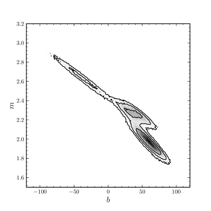
Once you have run an MCMC or equivalent and obtained a chain of samples from the posterior probability distribution for the full parameter set , you still must decide what to report about this sampling. A histogram of the samples in any one dimension is an approximation to the fully marginalized posterior probability distribution for that parameter, and in any two is that for the pair. You can find the “maximum a posteriori” (or MAP) value, by taking the peak of the marginalized posterior probability distribution for the line parameters . This, in general, will be different from the value at the peak of the unmarginalized probability distribution for all the parameters , because the posterior distribution can be very complex in the five-dimensional space. Because, for our purposes, the three parameters are nuisance parameters, it is more correct to take the “best-fit” from the marginalized distribution.
Of course finding the MAP value from a sampling is not trivial. At best, you can take the highest-probability sample. However, this works only for the unmarginalized distribution. The MAP value from the marginalized posterior probability distribution function for the two line parameters will not be the value of for the highest-probability sample. To find the MAP value in the marginalized distribution, it will be necessary to make a histogram or perform density estimation in the sample; this brings up an enormous host of issues way beyond the scope of this document. For this reason, we usually advise just taking the mean or median or some other simple statistic on the sampling. It is also possible to establish confidence intervals (or credible intervals) using the distribution of the samples.25
While the MAP answer—or any other simple “best answer”—is interesting, it is worth keeping in mind the third unfortunate thing about any Bayesian method: It does not return an “answer” but rather it returns a posterior probability distribution. Strictly, this posterior distribution function is your answer. However, what scientists are usually doing is not inference but rather decision-making. That is, the investigator wants a specific answer, not a distribution. There are (at least) two reactions to this. One is to ignore the fundamental Bayesianism at the end, and choose simply the MAP answer. This is the Bayesian’s analog of maximum likelihood; the standard uncertainty on the MAP answer would be based on the peak curvature or variance of the marginalized posterior distribution. The other reaction is to suck it up and sample the posterior probability distribution and carry forward not one answer to the problem but answers, each of which is drawn fairly and independently from the posterior distribution function. The latter is to be preferred because (a) it shows the uncertainties very clearly, and (b) the sampling can be carried forward to future inferences as an approximation to the posterior distribution function, useful for propagating uncertainty, or standing in as a prior for some subsequent inference.26 It is also returned, trivially (as we noted above) by the MCMC integrator we advised for performing the marginalization.
Exercise 5:
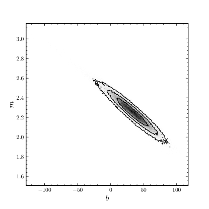
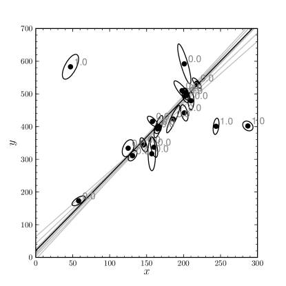
Using the mixture model proposed above—that treats the distribution as a mixture of a thin line containing a fraction of the points and a broader Gaussian containing a fraction of the points—find the best-fit (the maximum a posteriori) straight line for the , , and for the data in Table LABEL:table:data_allerr on page LABEL:table:data_allerr. Before choosing the MAP line, marginalize over parameters . That is, if you take a sampling approach, this means sampling the full five-dimensional parameter space but then choosing the peak value in the histogram of samples in the two-dimensional parameter space . Make one plot showing this two-dimensional histogram, and another showing the points, their uncertainties, and the MAP line. How does this compare to the standard result you obtained in Exercise 1? Do you like the MAP line better or worse? For extra credit, plot a sampling of 10 lines drawn from the marginalized posterior distribution for (marginalized over ) and plot the samples as a set of light grey or transparent lines. Your plot should look like Figure 4.
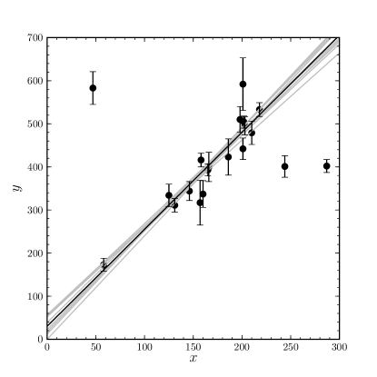
Exercise 6:
Solve Exercise 3 but now plot the fully marginalized (over ) posterior distribution function for parameter . Is this distribution peaked about where you would expect, given the data? Now repeat the problem, but dividing all the data uncertainty variances by 4 (or dividing the uncertainties by 2). Again plot the fully marginalized posterior distribution function for parameter . Your plots should look something like those in Figure 5. Discuss.
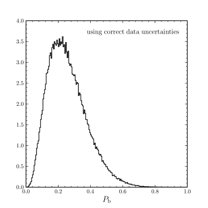
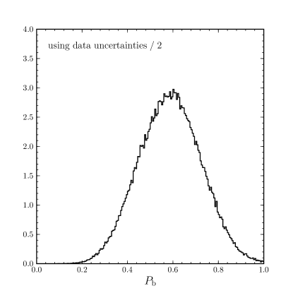
Section 4 Uncertainties in the best-fit parameters
In the standard linear-algebra method of minimization given in Section 1, the uncertainties in the best-fit parameters are given by the two-dimensional output covariance matrix
| (30) |
where the ordering is defined by the ordering in matrix . These uncertainties for the model parameters only strictly hold under three extremely strict conditions, none of which is met in most real situations: (a) The uncertainties in the data points must have variances correctly described by the ; (b) there must be no rejection of any data or any departure from the exact, standard definition of given in equation (19); and (c) the generative model of the data implied by the method—that is, that the data are truly drawn from a negligible-scatter linear relationship and subsequently had noise added, where the noise offsets were generated by a Gaussian process—must be an accurate description of the data.
These conditions are rarely met in practice. Often the noise estimates are rough (or missing entirely!), the investigator has applied data rejection or equivalent conditioning, and the relationship has intrinsic scatter and curvature.27 For these generic reasons, we much prefer empirical estimates of the uncertainty in the best-fit parameters.
In the Bayesian outlier-modeling schemes of Section 3, the output is a posterior distribution for the parameters . This distribution function is closer than the standard estimate to being an empirical measurement of the uncertainties of the parameters. The uncertainty variances and the covariance can be computed as second moments of this posterior distribution function. Computing the variances this way does involve assumptions, but it is not extremely sensitive to the assumption that the model is a good fit to the data; that is, as the model becomes a bad fit to the data (for example when the data points are not consistent with being drawn from a narrow, straight line), these uncertainties change in accordance. That is in strong contrast to the elements of the matrix , which don’t depend in any way on the quality of fit.
Either way, unless the output of the fit is being used only to estimate the slope, and nothing else, it is a mistake to ignore the off-diagonal terms of the uncertainty variance tensor. That is, you generally know some linear combinations of and much, much better than you know either individually (see, for example, Figures 4 and 6). When the data are good, this covariance is related to the location of the data relative to the origin, but any non-trivial propagation of the best-fit results requires use of either the full uncertainty tensor or else a two-dimensional sampling of the two-dimensional (marginalized, perhaps) posterior distribution.
In any non-Bayesian scheme, or when the full posterior has been discarded in favor of only the MAP value, or when data-point uncertainties are not trusted, there are still empirical methods for determining the uncertainties in the best-fit parameters. The two most common are bootstrap and jackknife. The first attempts to empirically create new data sets that are similar to your actual data set. The second measures your differential sensitivity to each individual data point.
In bootstrap, you do the unlikely-sounding thing of drawing data points randomly from the data points you have with replacement. That is, some data points get dropped, and some get doubled (or even tripled), but the important thing is that you select each of the that you are going to use in each trial independently from the whole set of you have. You do this selection of points once for each of bootstrap trials . For each of the trials , you get an estimate—by whatever method you are using (linear fitting, fitting with rejection, optimizing some custom objective function)—of the parameters , where goes from to . An estimate of your uncertainty variance on is
| (31) |
where stands for the best-fit using all the data. The uncertainty variance on is the same but with in the sum, and the covariance is the same but with . Bootstrap creates a new parameter, the number of trials. There is a huge literature on this, so we won’t say anything too specific, but one intuition is that once you have comparable to , there probably isn’t much else you can learn, unless you got terribly unlucky with your random number generator.
In jackknife, you make your measurement times, each time leaving out data point . Again, it doesn’t matter what method you are using, for each leave-one-out trial you get an estimate found by fitting with all the data except point . Then you calculate
| (32) |
and the uncertainty variance becomes
| (33) |
with the obvious modifications to make and . The factor accounts, magically, for the fact that the samples are not independent in any sense; this factor can only be justified in the limit that everything is Gaussian and all the points are identical in their noise properties.
Jackknife and bootstrap are both extremely useful when you don’t know or don’t trust your uncertainties . However, they do make assumptions about the problem. For example, they can only be justified when data represent a reasonable sampling from some stationary frequency distribution of possible data from a set of hypothetical, similar experiments. This assumption is, in some ways, very strong, and often violated.28 For another example, these methods will not give correct answers if the model does not fit the data reasonably well. That said, if you do believe your uncertainty estimates, any differences between the jackknife, bootstrap, and traditional uncertainty estimates for the best-fit line parameters undermine confidence in the validity of the model. If you believe the model, then any differences between the jackknife, bootstrap, and traditional uncertainty estimates undermine confidence in the data-point uncertainty variances .
Exercise 7:
Compute the standard uncertainty obtained for the slope of the line found by the standard fit you did in Exercise 1. Now make jackknife (20 trials) and bootstrap estimates for the uncertainty . How do the uncertainties compare and which seems most reasonable, given the data and uncertainties on the data?
Exercise 8:
Re-do Exercise 3—the mixture-based outlier model—but just with the “inlier” points 5 through 20 from Table LABEL:table:data_allerr on page LABEL:table:data_allerr. Then do the same again, but with all measurement uncertainties reduced by a factor of 2 (uncertainty variances reduced by a factor of 4). Plot the marginalized posterior probability distributions for line parameters in both cases. Your plots should look like those in Figure 6. Did these posterior distributions get smaller or larger with the reduction in the data-point uncertainties? Compare this with the dependence of the standard uncertainty estimate .
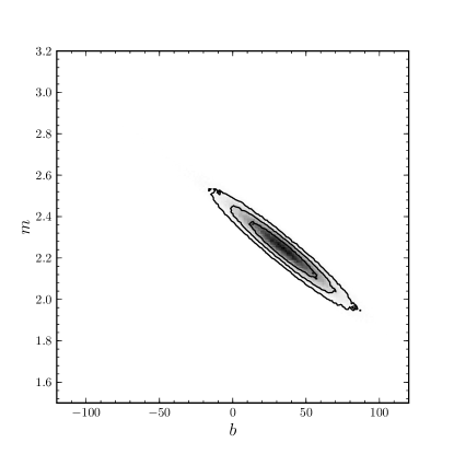
Section 5 Non-Gaussian uncertainties
The standard method of Section 1 is only justified when the measurement uncertainties are Gaussian with known variances. Many noise processes in the real world are not Gaussian; what to do? There are three general kinds of methodologies for dealing with non-Gaussian uncertainties. Before we describe them, permit an aside on uncertainty and error.
In note Notes, we point out that an uncertainty is a measure of what you don’t know, while an error is a mistake or incorrect value. The fact that a measurement differs from some kind of “true” value that it would have in some kind of “perfect experiment” can be for two reasons (which are not unrelated): It could be that there is some source of noise in the experiment that generates offsets for each data point away from its true value. Or it could be that the “measurement” is actually the outcome of some probabilistic inference itself and therefore comes with a posterior probability distribution. In either case, there is a finite uncertainty, and in both cases it comes somehow from imperfection in the experiment, but the way you understand the distribution of the uncertainty is different. In the first case, you have to make a model for the noise in the experiment. In the second, you have to analyze some posteriors. In either case, clearly, the uncertainty can be non-Gaussian.
All that said, and even when you suspect that the sources of noise are not Gaussian, it is still sometimes okay to treat the uncertainties as Gaussian: The Gaussian distribution is the maximum-entropy distribution for a fixed variance. That means that if you have some (perhaps magical) way to estimate the variance of your uncertainty, and you aren’t sure of anything else but the variance, then the Gaussian is—contrary to popular opinion—the most conservative thing you can assume.29 Of course it is very rare that you do know the variance of your uncertainty or noise; most simple uncertainty estimators are measurements of the central part of the distribution function (not the tails) and are therefore not good estimators of the total variance.
Back to business. The first approach to non-Gaussian noise or uncertainty is (somehow) to estimate the true or total variance of your uncertainties and then do the most conservative thing, which is to once again assume that the noise is Gaussian! This is the simplest approach, but rarely possible, because when there are non-Gaussian uncertainties, the observed variance of a finite sample of points can be very much smaller than the true variance of the generating distribution function. The second approach is to make no attempt to understand the non-Gaussianity, but to use the data-rejection methods of Section 3. We generally recommend data-rejection methods, but there is a third approach in which the likelihood is artificially or heuristically softened to reduce the influence of the outliers. This approach is not usually a good idea when it makes the objective function far from anything justifiable.30 The fourth approach—the only approach that is really justified—is to fully understand and model the non-Gaussianity.
For example, if data points are generated by a process the noise from which looks like a sum or mixture of Gaussians with different variances, and the distribution can be understood well enough to be modeled, the investigator can replace the Gaussian objective function with something more realistic. Indeed, any (reasonable) frequency distribution can be described as a mixture of Gaussians, so this approach is extremely general (in principle; it may not be easy). For example, the generative model in Section 2 for the standard case was built out of individual data-point likelihoods given in equation (21). If the frequency distribution for the noise contribution to data point has been expressed as the sum of Gaussians, these likelihoods become
| (34) |
where the Gaussians for measurement have variances , offsets (means—there is no need for the Gaussians to be concentric) , and amplitudes that sum to unity
| (35) |
In this case, fitting becomes much more challenging (from an optimization standpoint), but this can become a completely general objective function for arbitrarily complicated non-Gaussian uncertainties. It can even be generalized to situations of arbitrarily complicated joint distributions for all the measurement uncertainties.
One very common non-Gaussian situation is one in which the data points include upper or lower limits, or the investigator has a value with an uncertainty estimate but knows that the true value can’t enter into some region (for example, there are many situations in which one knows that all the true must be greater than zero). In all these situations—of upper limits or lower limits or otherwise limited uncertainties—the best thing to do is to model the uncertainty distribution as well as possible, construct the proper justified scalar objective function, and carry on.31 Optimization might become challenging, but that is an engineering problem that must be tackled for scientific correctness.
Section 6 Goodness of fit and unknown uncertainties
How can you decide if your fit is a good one, or that your assumptions are justified? And how can you infer or assess the individual data-point uncertainties if you don’t know them, or don’t trust them? These seem like different questions, but they are coupled: In the standard (frequentist) paradigm, you can’t test your assumptions unless you are very confident about your uncertainty estimates, and you can’t test your uncertainty estimates unless you are very confident about your assumptions.
Imagine that the generative model in Section 2 is a valid description of the data. In this case, the noise contribution for each data point has been drawn from a Gaussian with variance . The expectation is that data point will provide a mean squared error comparable to , and a contribution of order unity to when the parameters are set close to their true values. Because in detail there are two fit parameters which you have been permitted to optimize, the expectation for is smaller than . The model is linear, so the distribution of is known analytically and is given (unsurprisingly) by a chi-square distribution: in the limit of large the rule of thumb is that—when the model is a good fit, the uncertainties are Gaussian with known variances, and there are two linear parameters ( and in this case),
| (36) |
where the symbol is used loosely to indicate something close to a standard uncertainty (something close to a 68-percent confidence interval). If you find in this ballpark, it is conceivable that the model is good.32
Model rejection on the basis of too-large is a frequentist’s option. A Bayesian can’t interpret the data without a model, so there is no meaning to the question “is this model good?”. Bayesians only answer questions of the form “is this model better than that one?”. Because we are only considering the straight-line model in this document, further discussion of this (controversial, it turns out) point goes beyond our scope.33
It is easy to get a much higher than ; getting a lower value seems impossible; yet it happens very frequently. This is one of the many reasons that rejection or acceptance of a model on the basis is dangerous; exactly the same kinds of problems that can make unreasonably low can make it unreasonably high; worse yet, it can make reasonable when the model is bad. Reasons the value can be lower include that uncertainty estimates can easily be overestimated. The opposite of this problem can make high when the model is good. Even worse is the fact that uncertainty estimates are often correlated, which can result in a value significantly different from the expected value.
Correlated measurements are not uncommon; the process by which the observations were taken often involve shared information or assumptions. If the individual data-points have been estimated by some means that effectively relies on that shared information, then there will be large covariances among the data points. These covariances bring off-diagonal elements into the covariance matrix , which was trivially constructed in equation (16) under the assumption that all covariances (off-diagonal elements) are precisely zero. Once the off-diagonal elements are non-zero, must be computed by the matrix expression in equation (19); this is equivalent to replacing the sum over to two sums over and and considering all cross terms
| (37) |
where the are the elements of the inverse covariance matrix .
In principle, data-point uncertainty variance underestimation or mean point-to-point covariance can be estimated by adjusting them until is reasonable, in a model you know (for independent reasons) to be good. This is rarely a good idea, both because you rarely know that the model is a good one, and because you are much better served understanding your variances and covariances directly.
If you don’t have or trust your uncertainty estimates and don’t care about them at all, your best bet is to go Bayesian, infer them, and marginalize them out. Imagine that you don’t know anything about your individual data-point uncertainty variances at all. Imagine, further, that you don’t even know anything about their relative magnitudes; that is, you can’t even assume that they have similar magnitudes. In this case a procedure is the following: Move the uncertainties into the model parameters to get the large parameter list . Pick a prior on the uncertainties (on which you must have some prior information, given, for example, the range of your data and the like). Apply Bayes’s rule to obtain a posterior distribution function for all the parameters . Marginalize over the uncertainties to obtain the properly marginalized posterior distribution function for . No sane person would imagine that the procedure described here can lead to any informative inference. However, if the prior on the is relatively flat in the relevant region, the lack of specificity of the model when the uncertainties are large pushes the system to smaller uncertainties, and the inaccuracy of the model when the uncertainties are small pushes the system to larger uncertainties. If the model is reasonable, the inferred uncertainties will be reasonable too.
Exercise 9:
Exercise 10:
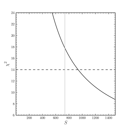
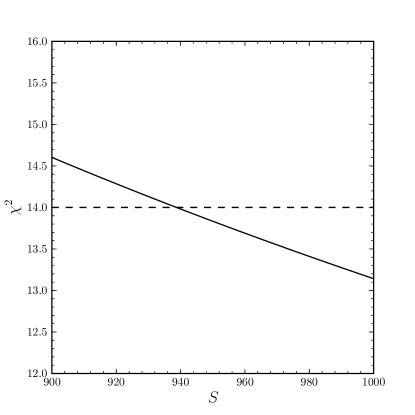
Re-do the fit of Exercise 1 but setting all , that is, ignoring the uncertainties and replacing them all with the same value . What uncertainty variance would make ? Relevant plots are shown in Figure 7. How does it compare to the mean and median of the uncertainty variances ?
Exercise 11:
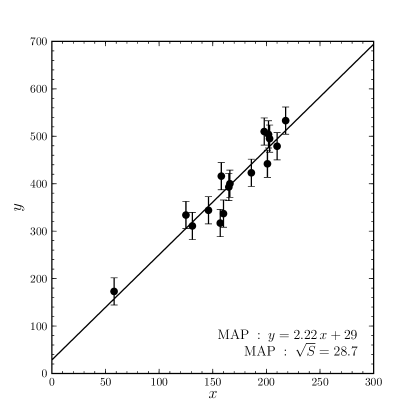
Flesh out and write all equations for the Bayesian uncertainty estimation and marginalization procedure described in this Section. Note that the inference and marginalization would be very expensive without excellent sampling tools! Make the additional (unjustified) assumption that all the uncertainties have the same variance to make the problem tractable. Apply the method to the and values for points 5 through 20 in Table LABEL:table:data_allerr on page LABEL:table:data_allerr. Make a plot showing the points, the maximum a posteriori value of the uncertainty variance as error bars, and the maximum a posteriori straight line. For extra credit, plot two straight lines, one that is maximum a posteriori for the full posterior and one that is the same but for the posterior after the uncertainty variance has been marginalized out. Your result should look like Figure 8. Also plot two sets of error bars, one that shows the maximum for the full posterior and one for the posterior after the line parameters have been marginalized out.

Section 7 Arbitrary two-dimensional uncertainties
Of course most real two-dimensional data come with uncertainties in both directions (in both and ). You might not know the amplitudes of these uncertainties, but it is unlikely that the values are known to sufficiently high accuracy that any of the straight-line fitting methods given so far is valid. Recall that everything so far has assumed that the -direction uncertainties were negligible. This might be true, for example, when the are the times at which a set of stellar measurements are made, and the are the declinations of the star at those times. It is not going to be true when the are the right ascensions of the star.
In general, when one makes a two-dimensional measurement , that measurement comes with uncertainties in both directions, and some covariance between them. These can be put together into a covariance tensor
| (38) |
If the uncertainties are Gaussian, or if all that is known about the uncertainties is their variances, then the covariance tensor can be used in a two-dimensional Gaussian representation of the probability of getting measurement when the “true value” (the value you would have for this data point if it had been observed with negligible noise) is :
| (39) |
where we have implicitly made column vectors
| (40) |
Now in the face of these general (though Gaussian) two-dimensional uncertainties, how do we fit a line? Justified objective functions will have something to do with the probability of the observations given the uncertainties , as a function of properties of the line. As in Section 2, the probability of the observations given model parameters is proportional to the likelihood of the parameters given the observations. We will now construct this likelihood and maximize it, or else multiply it by a prior on the parameters and report the posterior on the parameters.
Schematically, the construction of the likelihood involves specifying the line (parameterized by ), finding the probability of each observed data point given any true point on that line, and marginalizing over all possible true points on the line. This is a model in which each point really does have a true location on the line, but that location is not directly measured; it is, in some sense, a missing datum for each point.34 One approach is to think of the straight line as a two-dimensional Gaussian with an infinite eigenvalue corresponding to the direction of the line and a zero eigenvalue for the direction orthogonal to this. In the end, this line of argument leads to projections of the two-dimensional uncertainty Gaussians along the line (or onto the subspace that is orthogonal to the line), and evaluation of those at the projected displacements. Projection is a standard linear algebra technique, so we will use linear algebra (matrix) notation.35
A slope can be described by a unit vector orthogonal to the line or linear relation:
| (41) |
where we have defined the angle made between the line and the axis. The orthogonal displacement of each data point from the line is given by
| (42) |
where is the column vector made from in equation (40). Similarly, each data point’s covariance matrix projects down to an orthogonal variance given by
| (43) |
and then the log likelihood for or can be written as
| (44) |
where is some constant. This likelihood can be maximized, and the resulting values of are justifiably the best-fit values. The only modification we would suggest is performing the fit or likelihood maximization not in terms of but rather , where is the perpendicular distance of the line from the origin. This removes the paradox that the standard “prior” assumption of standard straight-line fitting treats all slopes equally, putting way too much attention on angles near . The Bayesian must set a prior. Again, there are many choices, but the most natural is something like flat in and flat in (the latter not proper).
The implicit generative model here is that there are points with true values that lie precisely on a narrow, linear relation in the – plane. To each of these true points a Gaussian offset has been added to make each observed point , where the offset was drawn from the two-dimensional Gaussian with covariance tensor . As usual, if this generative model is a good approximation to the properties of the data set, the method works very well. Of course there are many situations in which this is not a good approximation. In Section 8, we consider the (very common) case that the relationship is near-linear but not narrow, so there is an intrinsic width or scatter in the true relationship. Another case is that there are outliers; this can be taken care of by methods very precisely analogous to the methods in Section 3. We ask for this in the Exercises below.
It is true that standard least-squares fitting is easy and simple; presumably this explains why it is used so often when it is inappropriate. We hope to have convinced some readers that doing something justifiable and sensible when there are uncertainties in both dimensions—when standard linear fitting is inappropriate—is neither difficult nor complex. That said, there is something fundamental wrong with the generative model of this Section, and it is that the model generates only the displacements of the points orthogonal to the linear relationship. The model is completely unspecified for the distribution along the relationship.36
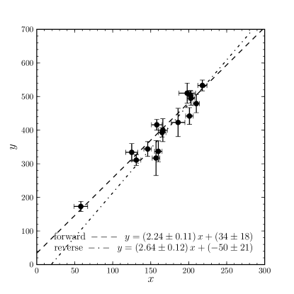
In the astrophysics literature (see, for example, the Tully–Fisher literature), there is a tradition, when there are uncertainties in both directions, of fitting the “forward” and “reverse” relations—that is, fitting as a function of and then as a function of —and then splitting the difference between the two slopes so obtained, or treating the difference between the slopes as a systematic uncertainty. This is unjustified.37 Another common method for finding the linear relationship in data when there are uncertainties in both directions is principal components analysis. The manifold reasons not to use PCA are beyond the scope of this document.38
Exercise 12:
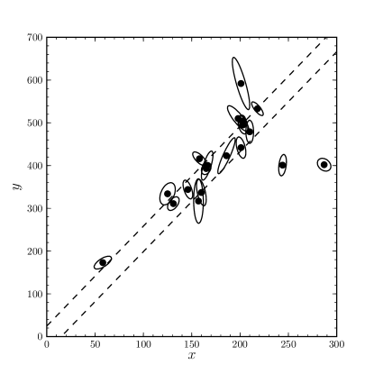
Using the method of this Section, fit the straight line to the , , , , and values of points 5 through 20 taken from Table LABEL:table:data_allerr on page LABEL:table:data_allerr. Make a plot showing the points, their two-dimensional uncertainties (show them as one-sigma ellipses), and the best-fit line. Your plot should look like Figure 9.
Exercise 13:
Repeat Exercise 7, but using all of the data in Table LABEL:table:data_allerr on page LABEL:table:data_allerr. Some of the points are now outliers, so your fit may look worse. Follow the fit by a robust procedure analogous to the Bayesian mixture model with bad-data probability described in Section 3. Use something sensible for the prior probability distribution for . Plot the two results with the data and uncertainties. For extra credit, plot a sampling of 10 lines drawn from the marginalized posterior distribution for and plot the samples as a set of light grey or transparent lines. For extra extra credit, mark each data point on your plot with the fully marginalized probability that the point is bad (that is, rejected, or has ). Your result should look like Figure 10.
Exercise 14:
Perform the abominable forward–reverse fitting procedure on points 5 through 20 from Table LABEL:table:data_allerr on page LABEL:table:data_allerr. That is, fit a straight line to the values of the points, using the -direction uncertainties only, by the standard method described in Section 1. Now transpose the problem and fit the same data but fitting the values using the -direction uncertainties only. Make a plot showing the data points, the -direction and -direction uncertainties, and the two best-fit lines. Your plot should look like Figure 11. Comment.
Exercise 15:
Perform principal components analysis on points 5 through 20 from Table LABEL:table:data_allerr on page LABEL:table:data_allerr. That is, diagonalize the matrix given by
| (45) |
| (46) |
Find the eigenvector of with the largest eigenvalue. Now make a plot showing the data points, and the line that goes through the mean of the data with the slope corresponding to the direction of the principal eigenvector. Your plot should look like Figure 12. Comment.
Section 8 Intrinsic scatter
So far, everything we have done has implicitly assumed that there truly is a narrow linear relationship between and (or there would be if they were both measured with negligible uncertainties). The words “narrow” and “linear” are both problematic, since there are very few problems in science, especially in astrophysics, in which a relationship between two observables is expected to be either. The reasons for intrinsic scatter abound; but generically the quantities being measured are produced or affected by a large number of additional, unmeasured or unmeasurable quantities; the relation between and is rarely exact, even in when observed by theoretically perfect, noise-free observations.
Proper treatment of these problems gets into the complicated area of estimating density given finite and noisy samples; again this is a huge subject so we will only consider one simple solution to the one simple problem of a relationship that is linear but not narrow. We will not consider anything that looks like subtraction of variances in quadrature; that is pure procedure and almost never justifiable.39 Instead—as usual—we introduce a model that generates the data and infer the parameters of that model.
Introduce an intrinsic Gaussian variance , orthogonal to the line. In this case, the parameters of the relationship become . In this case, each data point can be treated as being drawn from a projected distribution function that is a convolution of the projected uncertainty Gaussian, of variance defined in equation (43), with the intrinsic scatter Gaussian of variance . Convolution of Gaussians is trivial and the likelihood in this case becomes
| (47) |
where again is a constant, everything else is defined as it is in equation (44), and an additional term has appeared to penalize very broad variances (which, because they are less specific than small variances, have lower likelihoods). Actually, that term existed in equation (44) as well, but because there was no parameter, it did not enter into any optimization so we absorbed it into .
As we mentioned in note Notes, there are limitations to this procedure because it models only the distribution orthogonal to the relationship.40 Probably all good methods fully model the intrinsic two-dimensional density function, the function that, when convolved with each data point’s intrinsic uncertainty Gaussian, creates a distribution function from which that data point is a single sample. Such methods fall into the intersection of density estimation and deconvolution, and completely general methods exist.41
Exercise 16:
Re-do Exercise 7, but now allowing for an orthogonal intrinsic Gaussian variance and only excluding data point 3. Re-make the plot, showing not the best-fit line but rather the lines for the maximum-likelihood intrinsic relation. Your plot should look like Figure 13.
Exercise 17:
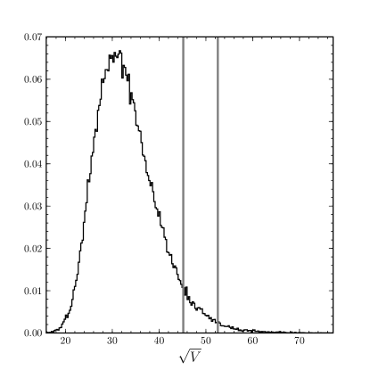
Re-do Exercise 8 but as a Bayesian, with sensible Bayesian priors on . Find and marginalize the posterior distribution over to generate a marginalized posterior probability for the intrinsic variance parameter . Plot this posterior with the 95 and 99 percent upper limits on marked. Your plot should look like Figure 14. Why did we ask only for upper limits?
Notes
1Copyyright 2010 by the authors. You may copy and distribute this document provided that you make no changes to it whatsoever.
2Above all we owe a debt to Sam Roweis (Toronto & NYU, now deceased), who taught us to find and optimize justified scalar objective functions. He will be sorely missed by all three of us. In addition it is a pleasure to thank Mike Blanton (NYU), Scott Burles (D. E. Shaw), Daniel Foreman-Mackey (Queens), Brandon C. Kelly (Harvard), Iain Murray (Edinburgh), Hans-Walter Rix (MPIA), and David Schiminovich (Columbia) for valuable comments and discussions. This research was partially supported by NASA (ADP grant NNX08AJ48G), NSF (grant AST-0908357), and a Research Fellowship of the Alexander von Humboldt Foundation. This research made use of the Python programming language and the open-source Python packages scipy, numpy, and matplotlib.
3When fitting is used for data-driven prediction—that is, using existing data to predict the properties of new data not yet acquired—the conditions for model applicability are weaker. For example, a line fit by the standard method outlined in Section 1 can be, under a range of assumptions, the best linear predictor of new data, even when it is not a good or appropriate model. A full discussion of this, which involves model selection and clarity about exactly what is being predicted (it is different to predict given than to predict given or and together), is beyond the scope of this document, especially since in astrophysics and other observational sciences it is relatively rare that data prediction is the goal of fitting.
4The term “linear regression” is used in many different contexts, but in the most common, they seem to mean “linear fitting without any use of the uncertainties”. In other words, linear regression is usually just the procedure outlined in this Section, but with the covariance matrix set equal to the identity matrix. This is equivalent to fitting under the assumption not just that the -direction uncertainties are negligible, but also that all of the -direction uncertainties are simultaneously identical and Gaussian.
Sometimes the term “linear regression” is meant to cover a much larger range of options; in our field of astrophysics there have been attempts to test them all (for example, see Isobe et al. 1990). This kind of work—testing ad hoc procedures on simulated data—can only be performed if you are willing to simultaneously commit (at least) two errors: First, the linear regression methods are procedures; they do not (necessarily) optimize anything that a scientist would care about. That is, the vast majority of procedures fail to produce a best-fit line in any possible sense of the word “best”. Of course, some procedures do produce a best-fit line under some assumptions, but scientific procedures should flow from assumptions and not the other way around. Scientists do not trade in procedures, they trade in objectives, and choose procedures only when they are demonstrated to optimize their objectives (we very much hope). Second, in this kind of testing, the investigator must decide which procedure “performs” best by applying the procedures to sets of simulated data, where truth—the true generative model—is known. All that possibly can be shown is which procedure does well at reproducing the parameters of the model with which the simulated data are generated! This has no necessary relationship with anything by which the real data are generated. Even if the generative model for the artificial data matches perfectly the generation of the true data, it is still much better to analyze the likelihood created by this generative model than to explore procedure space for a procedure that comes close to doing that by accident—unless, perhaps, when computational limitations demand that only a small number of simple operations be performed on the data.
5Along the lines of “egregious”, in addition to the complaints in the previous note, the above-cited paper (Isobe et al., 1990) makes another substantial error: When deciding whether to fit for as a function of or as a function of , the authors claim that the decision should be based on the “physics” of and ! This is the “independent variable” fallacy—the investigator thinks that is the independent variable because physically it “seems” independent (as in “it is really the velocity that depends on the distance, not the distance that depends on the velocity” and other statistically meaningless intuitions). The truth is that this decision must be based on the uncertainty properties of and . If has much smaller uncertainties, then you must fit as a function of ; if the other way then the other way, and if neither has much smaller uncertainties, then that kind of linear fitting is invalid. We have more to say about this generic situation in later Sections. What is written in Isobe et al. (1990)—by professional statisticians, we could add—is simply wrong.
6For getting started with modern data modeling and inference, the texts Mackay (2003), Press et al. (2007), and Sivia & Skilling (2006) are all very useful.
7Even in situations in which linear fitting is appropriate, it is still often done wrong! It is not unusual to see the individual data-point uncertainty estimates ignored, even when they are known at least approximately. It is also common for the problem to get “transposed” such that the coordinates for which uncertainties are negligible are put into the vector and the coordinates for which uncertainties are not negligible are put into the matrix. In this latter case, the procedure makes no sense at all really; it happens when the investigator thinks of some quantity “really being” the dependent variable, despite the fact that it has the smaller uncertainty. For example there are mistakes in the Hubble expansion literature, because many have an intuition that the “velocity depends on the distance” when in fact velocities are measured better, so from the point of view of fitting, it is better to think of the distance depending on the velocity. In the context of fitting, there is no meaning to the (ill-chosen) terms “independent variable” and “dependent variable” beyond the uncertainty or noise properties of the data. This is the independent variable fallacy mentioned in note Notes. In performing this standard fit, the investigator is effectively assuming that the values have negligible uncertainties; if they do not, then the investigator is making a mistake.
8As we mention in note Notes, scientific procedures should achieve justified objectives; this objective function makes that statement well posed. The objective function is also sometimes called the “loss function” in the statistics literature.
9The inverse covariance matrix appears in the construction of the objective function like a linear “metric” for the data space: It is used to turn a -dimensional vector displacement into a scalar squared distance between the observed values and the values predicted by the model. This distance can then be minimized. This idea—that the covariance matrix is a metric—is sometimes useful for thinking about statistics as a physicist; it will return in Section 7 when we think about data for which there are uncertainties in both the and directions.
Because of the purely quadratic nature of this metric distance, the standard problem solved in this Section has a linear solution. Not only that, but the objective function “landscape” is also convex so the optimum is global and the solution is unique. This is remarkable, and almost no perturbation of this problem (as we will see in later Sections) has either of these properties, let alone both. For this standard problem, the linearity and convexity permit a one-step solution with no significant engineering challenges, even when gets exceedingly large. As we modify (and make more realistic) this problem, linearity and convexity will both be broken; some thought will have to be put into the optimization.
10There is a difference between “uncertainty” and “error”: For some reason, the uncertainty estimates assigned to data points are often called “errors” or “error bars” or “standard errors”. That terminology is wrong: “They are uncertainties, not errors; if they were errors, we would have corrected them!” DWH’s mentor Gerry Neugebauer liked to say this; Neugebauer credits the quotation to physicist Matthew Sands. Data come with uncertainties, which are limitations of knowledge, not mistakes.
11In geometry or physics, a “scalar” is not just a quantity with a magnitude; it is a quantity with a magnitude that has certain transformation properties: It is invariant under some relevant transformations of the coordinates. The objective ought to be something like a scalar in this sense, because we want the inference to be as insensitive to coordinate choices as possible. The standard objective function is a scalar in the sense that it is invariant to translations or rescalings of the data in the vector space defined in equation (6). Of course a rotation of the data in the -dimensional space of the would be pretty strange, and would make the covariance matrix much more complicated, so perhaps the fact that the objective is literally a linear algebra scalar—this is clear from its matrix representation in equation (19)—is something of a red herring.
The more important thing about the objective is that it must have one magnitude only. Often when one asks scientists what they are trying to optimize, they say things like “I am trying to maximize the resolution, minimize the noise, and minimize the error in measured fluxes”. Well, those are good objectives, but you can’t optimize them all. You either have to pick one, or make a convex combination of them (such as by adding them together in quadrature with weights). This point is so obvious, it is not clear what else to say, except that many scientific investigations are so ill-posed that the investigator does not know what is being optimized. When there is a generative model for the data, this problem doesn’t arise.
12Of course, whether you are a frequentist or a Bayesian, the most scientifically responsible thing to do is not just optimize the objective, but pass forward a description of the dependence of the objective on the parameters, so that other investigators can combine your results with theirs in a responsible way. In the fully Gaussian case described in this Section, this means passing forward the optimum and second derivatives around that optimum (since a Gaussian is fully specified by its mode—or mean–and its second derivative at the mode). In what follows, when things aren’t purely Gaussian, more sophisticated outputs will be necessary.
13We have tried in this document to be a bit careful with words. Following Jaynes (2003), we have tried to use the word “probability” for our knowledge or uncertainty about a parameter in the problem, and “frequency” for the rate at which a random variable comes a particular way. So the noise process that sets the uncertainty has a frequency distribution, but if we are just talking about our knowledge about the true value of for a data point measured to have value , we might describe that with a probability distribution. In the Bayesian context, then—to get extremely technical—the posterior probability distribution function is truly a probability distribution, but the likelihood factor—really, our generative model—is constructed from frequency distributions.
14The likelihood has been defined in this document to be the frequency distribution for the observables evaluated at the observed data . It is a function of both the data and the model parameters. Although it appears as an explicit function of the data, this is called “the likelihood for the parameters” and it is thought of as a function of the parameters in subsequent inference. In some sense, this is because the data are not variables but rather fixed observed values, and it is only the parameters that are permitted to vary.
15One oddity in this Section is that when we set up the Bayesian problem we put the and into the prior information and not into the data. These were not considered data. Why not? This was a choice, but we made it to emphasize that in the standard approach to fitting, there is a total asymmetry between the and the . The are considered part of the experimental design; they are the input to an experiment that got the as output. For example, the are the times (measured by your perfect and reliable clock) at which you chose a priori to look through the telescope, and the are the declinations you measured at those times. As soon as there is any sense in which the are themselves also data, the method—Bayesian or frequentist—of this Section is invalid.
16It remains a miracle (to us) that the optimization of the objective, which is the only sensible objective under the assumptions of the standard problem, has a linear solution. One can attribute this to the magical properties of the Gaussian distribution, but the Gaussian distribution is also the maximum-entropy distribution (the least informative possible distribution) constrained to have zero mean and a known variance; it is the limiting distribution of the central limit theorem. That this leads to a convex, linear algebra solution is something for which we all ought to give thanks.
17Sigma clipping is a procedure that involves performing the fit, identifying the worst outliers in a sense—the points that contribute more than some threshold to the sum, removing those, fitting again, identifying again, and so on to convergence. This procedure is easy to implement, fast, and reliable (provided that the threshold is set high enough), but it has various problems that make it less suitable than methods in which the outliers are modeled. One is that sigma clipping is a procedure and not the result of optimizing an objective function. The procedure does not necessarily optimize any objective (let alone any justifiable objective). A second is that the procedure gives an answer that depends, in general, on the starting point or initialization, and because there is there is no way to compare different answers (there is no objective function), the investigator can’t decide which of two converged answers is “better”. You might think that the answer with least scatter (smallest per data point) is best, but that will favor solutions that involve rejecting most of the data; you might think the answer that uses the most data is best, but that can have a very large . These issues relate to the fact that the method does not explicitly penalize the rejection of data; this is another bad consequence of not having an explicit objective function. A third problem is that the procedure does not necessarily converge to anything non-trivial at all; if the threshold gets very small, there are situations in which all but two of the data points can be rejected by the procedure. All that said, with and standard, pretty good data, the sigma-clipping procedure is easy to implement and fast; we have often used it ourselves.
Complicating matters is the fact that sigma clipping is often employed in the common situation in which you have to perform data rejection but you don’t know the magnitudes of your uncertainties . We will say a bit more about this in Section 6, but a better procedure is to include the as (possibly restricted) model parameters and infer them and marginalize over them also. This is only really tractable if you can assume that all the data-point uncertainties are identical or you know something else equally informative about their relative magnitudes.
18Outlier modeling of this kind was used by Press (1997) to perform a meta-analysis of astronomical results, and is discussed at some length in a general way by Jaynes (2003).
19The exponential outlier model has a total of parameters, with data points: It has more parameters than data! Indeed, some would consider optimization or inference in this situation to be impossible. Of course it is not impossible, and for reasons that are instructive, though any detailed discussion is beyond the scope of this document. Fundamentally, optimization of this model is possible only when there are informative priors; in this case the informative prior is that all of the badness bits are integers, and every one of them can take on only the value zero or unity. This is a very strong prior, and limits the amount of information that can flow from the parameters of interest ( and ) into the uninteresting parameters . More generally, there is no limit on the number of parameters that can be constrained with a given data set; there is only a limit on the amount of information that those parameters can carry or obtain from the data. There is an additional subtlety, which goes way beyond the scope of this document, which is that the marginalization over the uninteresting parameters integrates out and thereby reduces the degeneracies.
20When flagging bad data, you might not want to give all points the same prior probability distribution function over , for example, when you combine data sets from different sources. Of course it is rare that one has reliable information about the unreliability of one’s data.
21One of the amusing things about the Bayesian posterior for the data rejections is that you can pick a particular data point and marginalize over and all the except . This will return the marginalized posterior probability that point is good. This is valuable for embarassing colleagues in meta-analyses (Press, 1997). Indeed, if embarassing colleagues is your goal, then Bayesian methods for data rejection are useful: They permit parameter-independent (that is, marginalized) statements about the probabilities that individual data points are bad. This is possible even in the marginalized mixture model: For any data point, at any setting of the parameters , the relative amplitude of the good and bad parts of the generative frequency distributions in equation (3) is the odds that the data point is bad (or good, depending on the direction of the ratio and one’s definition of the word “odds”). It is possible therefore to marginalize over all the parameters, obtaining the mean, for each data point , of the foreground frequency (mean taken over all samples from the posterior) evaluated at the data point and of the background frequency . The ratio of these is the marginalized odds that data point is bad.
22The likelihood—for example, that in equation (3)—is the likelihood “for the parameters” but it has units (or dimensions), in some sense, of inverse data, because it is computed as the probability distribution function for observations, evaluated at the observed data. The likelihood, therefore, is not something you can marginalize—the integral of the likelihood over a parameter has incomprehensible units. The posterior probability distribution function, on the other hand, has units (or dimensions) of inverse parameters, so it can be integrated over the parameter space. Marginalization, therefore, is only possible after construction of a posterior probability distribution function; marginalization is only possible in Bayesian analyses. This is related to the fact that the prior probability distribution function serves (in part) to define a measure in the parameter space. You can’t integrate without a measure.
If all you care about is parameters , and, furthermore, all you care about is the MAP answer, you must chose the MAP values from the marginalized posterior. This is because the MAP value of in the unmarginalized posterior will not, in general, have the same value of as the MAP value in the marginalized posterior. This point is important in many real cases of inference: Even small departures from Gaussianity in the posterior distribution function will lead to substantial shifts of the mode under marginalization. Of course, if what you are carrying forward is not the MAP result but a sampling from the posterior, a sampling from the unmarginalized posterior will contain the same distribution of values as a sampling from the marginalized one, by definition.
This document is not an argument in favor of Bayesian approaches; sometimes non-Bayesian approaches are much more expedient. What this document argues for is generative modeling, which is demanding. The standard objection to Bayesian methods is that they require priors, and those priors are hard (some say impossible) to set objectively. But this difficulty—in most problems of interest—pales in comparison to the difficulty of writing down a justifiable or even approximate generative model for the data.
While we claim to be neutral on Bayesianism relative to frequentism, there is one very important respect in which frequentists are at a disadvantage when there are nuisance parameters. If the nuisance parameters are powerful, and there are acceptable fits to the data that show a large range in the parameters of interest—as there will be in these mixture models when is made large—then a frequentist, who is not permitted to marginalize, will be able to conclude nothing interesting about the parameters of interest anywhere other than at the maximum-likelihood point. That is, the maximum-likelihood point might have a small and very good results for line parameters , but if the frequentist wants to be responsible and report the full range of models that is acceptable given the data, the frequentist must report that the data are also consistent with almost all the data being bad () and just about any line parameters you like. Marginalization stops this, because the specificity of the data explanation under small permits the small- regions of parameter space to dominate the marginalization integral. But if you have no measure (no prior), you can perform no marginalization, and the responsible party may be forced to report that no useful confidence interval on the line parameters are possible in this mixture model. That is a perfectly reasonable position, but demonstrates the cost of strict adherence to frequentism (which, for our purposes, is the position that there is no believable or natural measure or prior on the parameters).
23There is a good introduction to Metropolis–Hastings MCMC in Press et al. 2007, among other places.
24Variations of MCMC that go beyond Metropolis–Hastings—and the conditions under such variations make sense—are described in, for example, Gilks, Richardson, & Spiegelhalter (1995), Neal (2003), and Mackay (2003).
25Given a sampling of the posterior probability distribution function or the likelihood function of the parameters, it is most responsible to report—if not that entire sampling—some confidence intervals or credible intervals. There is a terminology issue in which the term “confidence interval” has become associated with frequentist statistics, which is unfortunate because Bayesian statistics is the calculus of plausibility or confidence. But whether you call them confidence intervals or credible intervals, the standard way to produce the confidence interval of fractional size ( for the 95 percent interval) on, say, your parameter , is as follows: Rank the samples in order of increasing and take either the smallest interval that contains a fraction of them, or else the interval which excludes the first and last of them. We usually do the latter, since it is fast and easy to explain. Then a good value to report is the median of the sampling, and quantiles around that median. But it does not matter much so long as the report is clear and sensible.
26Posterior probability distribution functions and samplings thereof are useful for propagating probabilistic information about a scientific result. However, they must be used with care: If the subsequent data analyzer has a prior that overlaps or conflicts with the prior used in making the posterior sampling, he or she will need access not just to the posterior probability distribution function but to the likelihood function. It is the likelihood function that contains all the information about the data—all the new information generated by the experiment—and therefore it is the likelihood that is most useful to subsequent users. Even a posterior sampling should be passed forward with likelihood or prior tags so that the prior can be divided out or replaced. Otherwise subsequent users live in danger of squaring (or worse) the prior.
27If you are sigma clipping or doing anything that looks like standard least-square fitting but with small modifications, it might be tempting to use the standard uncertainty estimate . But that is definitely wrong, because whatever encouraged you to do the sigma clipping or to make other modifications is probably sufficient reason to disbelieve the standard uncertainty estimate. In these cases you want either to be measuring the width of your posterior probability distribution function (if you are a Bayesian) or else using an empirical estimate of the uncertainty such as jackknife or bootstrap.
Bayesians like to be smug here—and have some justification—because the posterior distribution function gives the best fit parameters and the full distribution around that best-fit point in parameter space. However, the smugness must be tempered by the fact that within the context of a single model (such as the generative model described in Section 2), the Bayesian analysis does not return any useful goodness-of-fit information; a bad model can be constrained well by the data but still be dead wrong.
28Neither jackknife nor bootstrap make sense, in their naive forms, if there is a significant dynamic range in the uncertainty variances of the data points. This is because these techniques effectively treat all of the data equally. Of course, both methods could be adjusted to account for this; bootstrap could be made to randomly select points somehow proportionally to their contribution to the total inverse uncertainty variance (it is the sum of the that determines the total amount of information), and jackknife trials could be combined in a weighted way, weighted by the total inverse uncertainty variance. But these generalizations require significant research; probably the methods should be avoided if there is a large diversity in the .
29Assuming a Gaussian form is only conservative when you truly know the variance of the noise. Gaussians penalize heavily outliers, so they are not conservative in most situations. But if you included the outliers in your variance calculation, then it is conservative to make the Gaussian assumption. The issue is that it is almost impossible to make a variance estimate that captures the outliers properly.
30We don’t recommend them, but there are many non-Gaussian methods for removing sensitivity to outliers, which involve softening the objective function from (which depends quadratically on all residuals) to something that depends on large residuals to a smaller power. The most straightforward way to soften the objective function is to lower the power to which residuals are raised. For example, if we model the frequency distribution not with a Gaussian but rather with a biexponential
| (48) |
where is an estimate of the mean absolute uncertainty, probably correctly set to something like . Optimization of the total log likelihood is equivalent to minimizing
| (49) |
where is the straight line of equation 1. This approach is rarely justified, but it has the nice property that it introduces no new parameters. Another straightforward softening is to (smoothly) cut off the contribution of a residual as it becomes large. For example, replace with
| (50) |
where is the maximum amount a point can contribute to (Hampel et al., 1986). When each residual is small, its contribution to is nearly identical to its contribution to the standard , but as the residual gets substantial, the contribution of the residual does not increase as the square. This is about the simplest robust method that introduces only one new parameter (), and in principle, one can put a prior on , infer it, and marginalize it out. In general these are both far less good alternatives than modeling the outliers, because objective functions softer than are rarely justifiable in terms of any generative model for the data. In this Section we modeled outliers by a method that can almost be interpreted in terms of a softer ; in Section 5 we discuss (briefly) justifiable modifications to the objective function when the observational uncertainty distributions depart from Gaussians in known ways. Nonetheless, even when there is not a good justification for softening the objective function, it can sometimes be useful for generating a robust fit with a minimum of effort.
Along the same lines, sometimes it is justifiable to use Student’s -distribution for a softened objective. That is because the -distribution is what you get when you believe that the uncertainties are Gaussian, you don’t know their variances, but you imagine that the variances are drawn from some particular distribution (inverse chi-squared), and you marginalize.
31The possibility arises of having data points that are not true measurements but only, for example, upper limits. In most contexts (in astrophysics, anyway) an “upper limit” is caused by one of two things. Either the investigator has taken the logarithm of a quantity that in fact, for some measurements, went to zero or negative; or else the investigator is fitting a model to a binned quantity and in some bins there are no objects or data. In the first case, the best advice is not to take the logarithm at all. Fit a power-law or exponential in the linear space rather than a straight line in the log space. In the second case, the best advice is to use the likelihood appropriate for a Poisson process rather than a Gaussian process. Least-square fitting is an approximation when the data are generated by a Poisson sampling; this approximation breaks down when the number of objects per bin becomes small. Optimizing the correct Poisson likelihood is not difficult, and it is the only scientifically justifiable thing to do.
It is rare that there are true upper limits not caused by one of the above. However, if neither of the above applies—perhaps because the investigator was given only the limits, and not the details of their origins—the right thing to do is to write down some generative model for the limits. This would be some description of the “probability of the data given the model” where the (say) 95-percent upper limit is replaced with a probability distribution that has 95 percent of its mass below the reported limit value. This is ideally done with a correct model of the measurement process, but it is acceptable in cases of justifiable ignorance to make up something reasonable; preferably something that is close to whatever distribution maximizes the entropy given the reported and logical constraints.
32Frequentist model rejection on the basis of unacceptable should not be confused with model comparison performed with . If differs from the number of degrees of freedom by something on the order of , the model cannot be rejected on a basis. However, if two equally plausible models differ from one another by a difference substantially larger than unity, the model with the lower can be preferred and the higher rejected on that basis, even if the higher still shows an acceptable . This difference between model rejection and model comparison is counterintuitive, but it emerges from the difference that in the model comparison case, there are two models, not one, and they are both (by assumption) equally plausible a priori. The conditions for model comparison are fairly strong, so the test is fairly sensitive. In the case of correctly estimated uncertainty variances and two models that are equally plausible a priori, the value between the models is (twice) the natural logarithm of the odds ratio between the models. For this reason, large values generate considerable confidence.
33Technically, Bayesians cannot reject a model outright on the basis of bad alone; Bayesians can only compare comparable models. A Bayesian will only consider the absolute value of to provide hints about what might be going wrong. Part of the reason for this is that a Bayesian analysis returns a probability distribution over mutually exclusive hypotheses. This distribution or this set of probabilities integrates or sums to unity. If only one model (“the data are drawn from a straight line, plus noise”) is considered, the probabilities for the parameters of that model will integrate to unity and the model cannot be disfavored in any sense. Of course, any time an investigator considers only one model, he or she is almost certainly making a mistake, and any conservative Bayesian data analyst will consider a large space of models and ask about the evidence for the alternatives, or for complexification of the current model. So a Bayesian can reject models on a basis—provided that he or she has permitted a wide enough range of models, and provided those models have somewhat comparable prior probabilities. Model rejection and hypothesis comparison are large topics that go beyond the scope of this document.
Many Bayesians argue that they can reject models without alternatives, by, for example, comparing likelihood (or Bayes factor—the likelihood integrated over the prior) under the data and under artificial data generated with the same model (with parameters drawn from the prior). This is true, and it is a good idea for any Bayesian to perform this test, but there is still no correct proababilistic statement that can be made about model rejection in the single-model situation (you can’t reject your only model).
In general, the investigator’s decision-making about what models to consider (which will be informed by tests like comparisons between likelihoods and fake-data likelihoods) have an enormous impact on her or his scientific conclusions. At the beginning of an investigation, this problem lies in the setting of priors. An investigator who considers only a straight-line model for her or his points is effectively setting insanely informative priors—the prior probability of every alternative model is precisely zero! At the end of an investigation, this problem—what models to report or treat as confirmed—lies in the area of decision theory, another topic beyond the scope of this document. But even in a context as limited as straight-line fitting, it is worth remembering that, as scientists, we are not just inferring things, we are making decisions—about what is right and wrong, about what to investigate, about what to report, and about what to advocate—and these decisions are only indirectly related to the inferences we perform.
34One amusing aspect of the generative model we are about to write down is that it is possible to marginalize it over all the parameters and all the true positions of the points along the linear relationship except for one and thereby produce a marginalized posterior probability distribution function for the true position of any individual data point, under the assumptions of the generative model. That is, it is possible to reconstruct the missing data.
35The fact that the marginalization over the true positions of the points reduces to a projection along the line—or onto the subspace orthogonal to the line—makes this method very similar to that called “orthogonal least squares”. This generative model justifies that procedure, in the case when the orthogonal displacements are penalized by the properly projected uncertainties.
36This probably means that although this two-dimensional fitting method works, there is something fishy or improper involved. The model is only strictly correct, in some sense, when the distribution along the line is uniform over the entire range of interest. That’s rarely true in practice.
37The difference between the forward-fitting and reverse-fitting slopes is a systematic uncertainty in the sense that if you are doing something unjustifiable you will certainly introduce large systematics! This forward–reverse procedure is not justifiable and it gives results which differ by substantially more than the uncertainty in the procedure given in this Section. We have already (note Notes) criticized one of the principal papers to promote this kind of hack, and do not need to repeat that criticism here.
38Why not use principal components analysis? In a nutshell: The method of PCA does return a linear relationship for a data set, in the form of the dominant principal component. However, this is the dominant principal component of the observed data, not of the underlying linear relationship that, when noise is added, generates the observations. For this reason, the output of PCA will be strongly drawn or affected by the individual data point noise covariances . This point is a subtle one, but in astrophysics it is almost certainly having a large effect in the standard literature on the “fundamental plane” of elliptical galaxies, and in other areas where a fit is being made to data with substantial uncertainties. Of course PCA is another trivial, linear method, so it is often useful despite its inapplicability; and it becomes applicable in the limit that the data uncertainties are negligible (but in that case everything is trivial anyway).
39The standard method for estimating the width of a linear relationship is to compare the scatter of the data points to the scatter expected if the relationship is narrow. The estimated intrinsic scatter can be “found” in this case by a procedure of subtracting in quadrature (intrinsic variance is observed variance minus expected variance given observational uncertainties). This is not a good idea in general. It doesn’t work at all if the data points have a significant dynamic range in their measurement uncertainties, it can produce an estimate of the intrinsic scatter variance that is negative, and it returns no confidence interval or uncertainty. In the case of negligible -direction uncertainties, a better method is to add a parameter which is a variance to be added in quadrature to every data-point uncertainty variance; this is what we advocate in the main text.
40One confusing issue in the subject of intrinsic scatter is the direction for the scatter. If things are Gaussian, it doesn’t matter whether you think of the scatter being in the direction, the direction, or the direction perpendicular to the line (as we think of it in the method involving in this Section). However it must be made clear which direction is being used for the statement of the result, and what the conversions are to the other directions (these involve the angle or slope of course).
References
- Bovy, Hogg, & Roweis (2009) Bovy, J., Hogg, D. W., & Roweis, S. T., 2009, Extreme deconvolution: inferring complete distribution functions from noisy, heterogeneous, and incomplete observations, arXiv:0905.2979 [stat.ME]
- Jaynes (2003) Jaynes, E. T., 2003, Probability theory: the logic of science (Cambridge University Press)
- Gilks, Richardson, & Spiegelhalter (1995) Gilks, W. R., Richardson, S., & Spiegelhalter, D., 1995, Markov chain Monte Carlo in practice: interdisciplinary statistics (Chapman & Hall/CRC)
- Hampel et al. (1986) Hampel, F. R., Ronchetti, E. M., Rousseeuw, P. J., & Stahel, W. A., 1986, Robust statistics: the approach based on influence functions (New York: Wiley)
- Isobe et al. (1990) Isobe, T., Feigelson, E. D., Akritas, M. G., & Babu, G. J., 1990, Linear regression in astronomy, Astrophysical Journal 364 104
- Kelly (2007) Kelly, B. C., 2007, Some aspects of measurement error in linear regression of astronomical data, Astrophysical Journal 665 1489
- Mackay (2003) Mackay, D. J. C., 2003, Information theory, inference, and learning algorithms (Cambridge University Press)
- Neal (2003) Neal., R. M., 2003, Slice sampling, Annals of Statistics, 31(3), 705
- Press (1997) Press, W. H., 1997, Understanding data better with Bayesian and global statistical methods, in Unsolved problems in astrophysics, eds. Bahcall, J. N. & Ostriker, J. P. (Princeton University Press) 49–60
- Press et al. (2007) Press, W. H., Teukolsky, S. A., Vetterling, W. T., & Flannery, B. P., 2007, Numerical recipes: the art of scientific computing (Cambridge University Press)
- Sivia & Skilling (2006) Sivia, D. S. & Skilling, J., 2006, Data analysis: a Bayesian tutorial (Oxford University Press)