Exclusive Queueing Process with Discrete Time

Abstract

In a recent study [2], an extension of the M/M/1 queueing process with the excluded-volume effect as in the totally asymmetric simple exclusion process (TASEP) was introduced. In this paper, we consider its discrete-time version. The update scheme we take is the parallel one. A stationary-state solution is obtained in a slightly arranged matrix product form of the discrete-time open TASEP with the parallel update. We find the phase diagram for the existence of the stationary state. The critical line which separates the parameter space into regions with and without the stationary state can be written in terms of the stationary current of the open TASEP. We calculate the average length of the system and the average number of particles.

1 Introduction

The queueing theory has been considerably studied since Erlang started designing telephone exchanging system in 1909 [9]. In [10], he developed the theory of the call-loss system, which significantly contributed to the progress of telephones and electric communication systems. After his study, Kendall presented his first paper [16]. Since then, the study on the queueing theory including Kendall’s notation [17], Burke’s theorem [5], Jackson networks [14], and Little’s theorem [20] has been accelerated. Nowadays, it is applied to study on social systems such as the Internet [21], resource management systems [3], vehicular traffic systems [13] and pedestrian traffic systems [12].

Let us review here the discrete-time M/M/1 queueing process, which will be extended in the next section.

Figure 1: M/M/1 queueing process.

M/M/1 means that the queue has a Markovian entry of customers and a Markovian exit at 1 server. Each particle (customer) enters the system with a probability $\alpha$ and receives service with a probability $\beta$, see figure 1. The system is characterized only by the number $N\in{\mathbb{Z}}_{\geq 0}$ of particles. The probability $P(N;t)$ of finding $N$ particles at time $t$ is governed by the following master equation:

$$P(0;t+1)= (1-\alpha)P(0;t)+\alpha\beta P(0;t)+(1-\alpha)\beta P(1;t),$$ (1)

$$\begin{split}P(N;t+1)=&\alpha(1-\beta)P(N-1;t)+(1-\alpha)(1-\beta)P(N;t)\\ &+\alpha\beta P(N;t)+(1-\alpha)\beta P(N+1;t),\end{split}$$ (2)

for $N\in{\mathbb{N}}$. When $\alpha<\beta$, a unique stationary-state solution to the master equation can be easily obtained as the following geometric distribution:

$$P(N)=\frac{\beta-\alpha}{\beta(1-\alpha)}\left(\frac{\alpha(1-\beta)}{(1-\alpha)\beta}\right)^{N}.$$ (3)

The average number of particles can be easily calculated as

$$\langle N\rangle=\sum_{N=1}^{\infty}N\frac{\beta-\alpha}{\beta(1-\alpha)}\left(\frac{\alpha(1-\beta)}{(1-\alpha)\beta}\right)^{N}=\frac{\alpha(1-\beta)}{\beta-\alpha}.$$ (4)

On the other hand, the asymmetric simple exclusion process (ASEP) in one dimension is one of typical interacting particle systems and admits exact analyses of non-equilibrium properties [19, 25]. It has been vigorously studied in the recent two decades. The stationary state of the totally ASEP with open boundaries (open TASEP) was found in a matrix product form in [8]. Since then, matrix product stationary states of various generalizations of the ASEP containing discrete-time versions of the open TASEP have been found [4]. The TASEP is one of the basic models of the vehicular traffic [7].

Although both the M/M/1 queueing process and the open TASEP are Markov processes with particle entry and exit, they are different in the following two points. First, the number of particles in the M/M/1 queueing process does not have an upper limit, whereas that in the open TASEP cannot be greater than the fixed number of sites. In other words, the state space of the M/M/1 queueing process is infinite and that of the open TASEP is finite. It should be noticed that the open TASEP is a call-loss system, which has been seldom discussed. Second, the TASEP has a spatial structure, and particles are affected by their excluded volume (hard-core repulsion). By contrast, the M/M/1 queueing process has no spatial structure, and only the number of particles characterizes the system.

An extension of the M/M/1 queueing process with the excluded-volume effect (in other words, the TASEP with a new boundary condition) was introduced in [2]. In this model, particles enter the system at the left site next to the leftmost occupied site and exit at the rightmost site of the chain, see Fig. 2. When we (pedestrians) make a queue, we usually proceed if there is a space in front of us (excluded-volume effect), which is a motivation to treat this model. Let us call the model exclusive queueing process.

In [2], a stationary state of the exclusive queueing process was given by a slightly arranged matrix product form for the open TASEP, where the probability of finding each configuration is proportional to

$$c^{L}\times\langle\text{row vector}|\text{ matrix product }|\text{column vector}\rangle.$$ (5)

The row vector, the matrices and the column vector are independent of the entry rate $\alpha$, whereas $c$ is independent of the exit rate $\beta$. The exponent $L$ denotes the position of the leftmost particle.

In this paper, we consider a discrete-time version of the exclusive queueing process with the entry, hopping and exit rates ($\alpha,p$ and $\beta$, respectively) replaced by probabilities within one time step. Although there are some choices of an update scheme, we take the fully-parallel-update rule. The special case where the bulk hopping is deterministic (i.e., the hopping probability is 1) has been analyzed in [26].

To find a stationary-state solution is one of basic problems. The idea to find it in this paper is reducing the balance equation for the exclusive queueing process to that for the open TASEP. Then, a stationary-state solution will be obtained in a similar form to that for the continuous-time model as (5). We calculate the critical line which separates the parameter space into the regions with and without the stationary state by evaluating the convergence of the normalization constant. The critical line will be written in terms of the stationary current of the open TASEP. We calculate the average length of the system (the position of the leftmost particle) and the average number of particles in the system. We also calculate the average number of particles in the queue.

Figure 2: Exclusive queueing process.

This paper is organized as follows. In Sect. 2, we define the exclusive queueing process with discrete time. In Sect. 3, we obtain a stationary state of the model. In Sect. 4, we identify the region where the stationary state exists in the parameter space, and calculate the average length of the system and the average number of particles. In Sect. 5, we treat the model in the case where the bulk hopping probability is 1. Section 6 is devoted to the conclusion of this paper. Detailed calculations are done in Appendices.

2 Model

We introduce an extension of the discrete-time M/M/1 queueing process with the excluded-volume effect on the semi-infinite chain (exclusive queueing process), see Fig. 2, where each site is labeled by a natural number from right to left. Each particle enters the chain at the left site next to the leftmost occupied site with a probability $\alpha$, hops to its right nearest neighbor site with a probability $p$, if it is empty, and exits at the right end of the chain with a probability $\beta$. If there is no particle on the chain, a particle enters at site 1. These transitions occur simultaneously within one time step. In other words, we take the fully-parallel-update scheme. (We call it simply parallel update hereafter.) The model is formulated as a discrete-time Markov process on the state space $S=\{\emptyset,1,10,11,100,101,110,111,1000,\dots\}$ where 0 and 1 correspond to unoccupied and occupied sites, respectively. In particular, $\emptyset$ denotes the state that there is no particle on the chain. Note that we do not write infinite 0s located left to the leftmost 1. We define $|\tau|$ by the length of a sequence $\tau$. In particular, for each element $\tau$ of $S$, $|\tau|$ stands for the length of the system (the position of the leftmost occupied site). Let us write the probability of finding a configuration $\tau$ at time $t$ as $P(\tau;t)$. The master equation governing the model is written as

$$P(\tau;t+1)={\mathcal{T}}P(\tau;t)=\sum_{\tau^{\prime}\in S}W(\tau^{\prime}\to\tau)P(\tau^{\prime};t),$$ (6)

where ${\mathcal{T}}$ is the transition-probability matrix of the process and $W(\tau^{\prime}\to\tau)$ is the transition probability from $\tau^{\prime}$ to $\tau$ within one time step. In particular, for $\tau=\emptyset$ and $\tau=1$,

$$P(\emptyset;t+1)=(1-\alpha)P(\emptyset;t)+(1-\alpha)\beta P(1;t),$$ (7)

$$P(1;t+1)=\alpha P(\emptyset;t)+(1-\alpha)(1-\beta)P(1;t)+(1-\alpha)pP(10;t).$$ (8)

It is difficult to write down the action of ${\mathcal{T}}$ explicitly for the general configuration $\tau$ because of the parallel update. For example, for $\tau=101101$,

$$\begin{split}&\!\!\!\!\!\!P(101101;t+1)\\ =&(1-\alpha)(1-p)^{2}(1-\beta)P(101101;t)+(1-\alpha)(1-p)pP(101110;t)\\ &+(1-\alpha)p(1-p)(1-\beta)P(110101;t)\\ &+(1-\alpha)p(1-p)(1-\beta)P(1001101;t)+(1-\alpha)p^{2}P(110110;t)\\ &+(1-\alpha)p^{2}P(1001110;t)+(1-\alpha)p^{2}(1-p)(1-\beta)P(1010101;t)\\ &+(1-\alpha)p^{3}P(1010110;t)+\alpha p^{2}P(10110;t)\\ &+\alpha p(1-p)(1-\beta)P(10101;t),\end{split}$$ (9)

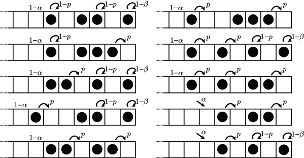
see Fig. 3, and for $\tau=100100$,

$$\begin{split}&\!\!\!\!\!\!P(100100;t+1)\\ =&(1-\alpha)(1-p)^{2}P(100100;t)+(1-\alpha)(1-p)pP(101000;t)\\ &+(1-\alpha)p(1-p)P(1000100;t)+(1-\alpha)p^{2}P(1001000;t)\\ &+(1-\alpha)(1-p)^{2}\beta P(100101;t)+(1-\alpha)(1-p)p\beta P(101001;t)\\ &+(1-\alpha)p(1-p)\beta P(1000101;t)+(1-\alpha)p^{2}\beta P(1001001;t),\end{split}$$ (10)

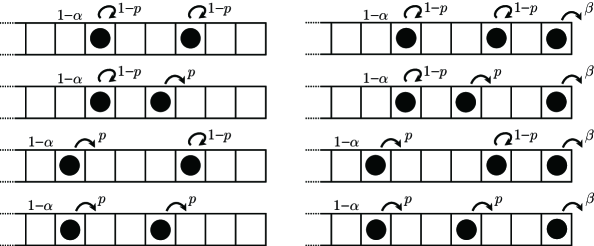
see Fig. 4.

Figure 3: List of all configurations which transit to $101101$ with a non-zero probability within one time step.

Figure 4: List of all configurations which transit to $100100$ with a non-zero probability within one time step.

Note that this model is not equivalent to the parallel-update TASEP with the ordinary open boundary condition (open TASEP) [11], see Fig. 5.

Figure 5: TASEP with the ordinary open boundary condition.

In the open TASEP, particles can enter the system at the fixed leftmost site of the finite chain only if it is empty. This means that the open TASEP is a call-loss system. On the other hand, in our model, particles can always enter the system.

3 Stationary state

A stationary state (stationary distribution) is a solution to the balance equation

$$P(\tau)={\mathcal{T}}P(\tau)\ (\forall\tau\in S)$$ (11)

with the constraint

$$\sum_{\tau\in S}P(\tau)=1.$$ (12)

Let us begin with making an assumption that the stationary-state solution has the following form:

$$P(\emptyset)= \frac{1}{Z},$$ (13)

$$P(1\tau_{L-1}\dots\tau_{1})= \frac{1}{Z}\left(\frac{\alpha}{p(1-\alpha)}\right)^{L}f_{L}(1\tau_{L-1}\dots\tau_{1}),$$ (14)

where $f_{L}$ is a function on $\{0,1\}^{L}$ and satisfies

$$f_{L}(101\tau) =f_{L-1}(11\tau)+pf_{L-2}(1\tau),$$ (15)

$$f_{L}(100\tau) =(1-p)f_{L-1}(10\tau),$$ (16)

$$f_{L}(01\tau) =pf_{L-1}(1\tau),$$ (17)

$$f_{L}(00\tau) =0.$$ (18)

From $P(\emptyset)={\mathcal{T}}P(\emptyset)$, we get

$$P(1)=\frac{1}{Z}\frac{\alpha}{p(1-\alpha)}\frac{p}{\beta}.$$ (19)

From $P(1)={\mathcal{T}}P(1)$, we get

$$P(10)=\frac{1}{Z}\left(\frac{\alpha}{p(1-\alpha)}\right)^{2}\frac{p}{\beta}.$$ (20)

Thus,

$$f_{1}(1)=\frac{p}{\beta},$$ (21)

$$f_{2}(10)=\frac{p}{\beta}.$$ (22)

We reduce the balance equation for the general configuration to that for the open TASEP. One can obtain, for all $11\tau\in S$ with length $L$,

$$\begin{split}f_{L}(11\tau)=&\sum_{\tau^{\prime}\in{\mathcal{A}}_{11}(\tau)}\frac{1}{1-\alpha}W(11\tau^{\prime}\to 11\tau)f_{L}(11\tau^{\prime})\\ &+\sum_{\tau^{\prime}\in{\mathcal{A}}_{11}(\tau)}\frac{1}{\alpha}W(1\tau^{\prime}\to 11\tau)f_{L}(01\tau^{\prime}),\end{split}$$ (23)

for all $101\tau\in S$ with length $L$,

$$\begin{split}f_{L}(101\tau)=&\sum_{\tau^{\prime}\in{\mathcal{A}}_{101}(\tau)}\frac{1}{1-\alpha}W(101\tau^{\prime}\to 101\tau)f_{L}(101\tau^{\prime})\\ &+\sum_{\tau^{\prime}\in{\mathcal{A}}_{101}(\tau)}\frac{1}{1-\alpha}W(110\tau^{\prime}\to 101\tau)f_{L}(110\tau^{\prime})\\ &+\sum_{\tau^{\prime}\in{\mathcal{A}}_{101}(\tau)}\frac{1}{\alpha}W(10\tau^{\prime}\to 101\tau)f_{L}(010\tau^{\prime}),\end{split}$$ (24)

and for all $100\tau\in S$ with length $L$,

$$\begin{split}f_{L}(100\tau)=&\sum_{\tau^{\prime}\in{\mathcal{A}}_{100}(\tau)}\frac{1}{1-\alpha}W(10\tau^{\prime}\to 100\tau)f_{L}(10\tau^{\prime})\\ &+\sum_{\tau^{\prime}\in{\mathcal{A}}_{100}(\tau)}\frac{1}{(1-\alpha)(1-p)}W(10\tau^{\prime}\to 100\tau)f_{L}(00\tau^{\prime}),\end{split}$$ (25)

see Appendix A for detailed calculation. The sets ${\mathcal{A}}_{\dots}(\tau)$ are defined as

$${\mathcal{A}}_{11}(\tau):= \{\tau^{\prime}|W(11\tau^{\prime}\to 11\tau)>0\wedge|\tau|=|\tau^{\prime}|\},$$ (26)

$${\mathcal{A}}_{101}(\tau):= \{\tau^{\prime}|W(101\tau^{\prime}\to 101\tau)>0\wedge|\tau|=|\tau^{\prime}|\},$$ (27)

$${\mathcal{A}}_{100}(\tau):= \{\tau^{\prime}|W(10\tau^{\prime}\to 100\tau)>0\wedge|\tau|=|\tau^{\prime}|-1\}.$$ (28)

For example,

$${\mathcal{A}}_{11}(0110) =\{0110,1010,0111,1011\},$$ (29)

$${\mathcal{A}}_{101}(110) =\{110,111\},$$ (30)

$${\mathcal{A}}_{100}(110) =\{0110,1010,0111,1011\}.$$ (31)

Equations (23)-(25) give the balance equation for the open TASEP on the $L$-site chain with the entry probability equal to 1 if we regard $f_{L}(\tau)$ as the probability of finding a configuration $\tau$. Thus, if we set $f_{L}$ to be proportional to the stationary-state solution to the open TASEP, the form (13) and (14) gives a stationary-state solution to our model. Substituting the matrix product solution to the open TASEP which was found in [11] into (14), we obtain

$$P(\tau)=\begin{cases}\frac{1}{Z}&\tau=\emptyset,\\ \frac{1}{Z}\left(\frac{\alpha}{p(1-\alpha)}\right)^{L}\langle W|DX_{\tau_{L-1}}\cdots X_{\tau_{1}}|V\rangle&\tau=1\tau_{L-1}\dots\tau_{1},\end{cases}$$ (32)

where $X_{1}=D$ and $X_{0}=E$ are matrices, $\langle W|$ is a row vector and $|V\,\rangle$ is a column vector. They should satisfy

$$\begin{split}EDEE=&(1-p)EDE+EEE+pEE,\\ EDED=&EDD+EED+pED,\\ DDEE=&(1-p)DDE+(1-p)DEE+p(1-p)DE,\\ DDED=&DDD+(1-p)DED+pDD,\\ DDE|V\,\rangle=&(1-\beta)DD|V\,\rangle+(1-p)DE|V\,\rangle+p(1-\beta)D|V\,\rangle,\\ EDE|V\,\rangle=&(1-\beta)ED|V\,\rangle+EE|V\,\rangle+pE|V\,\rangle,\\ \langle W|DEE=&(1-p)\langle W|DE,\\ \langle W|DED=&\langle W|DD+p\langle W|D,\\ DD|V\,\rangle=&\frac{p(1-\beta)}{\beta}D|V\,\rangle,\\ ED|V\,\rangle=&\frac{p}{\beta}E|V\,\rangle,\\ \langle W|EE=&0,\\ \langle W|ED=&p\langle W|D,\end{split}$$ (33)

which is the algebraic relation found in [11] with $\alpha=1$. This algebraic relation is compatible with the assumption (15)-(18). A representation of the relation is given in Appendix B. In view of (21), we have to chose the normalization as

$$\langle W|D|V\,\rangle=\frac{p}{\beta}.$$ (34)

Note that, from the algebraic relation, we can derive $\langle W|DE|V\,\rangle=\frac{p}{\beta}$, which is compatible with (22). The normalization constant $Z$ is expressed as

$$Z=1+\sum_{L\geq 1}\left(\frac{\alpha}{p(1-\alpha)}\right)^{L}\langle W|D(D+E)^{L-1}|V\,\rangle$$ (35)

when the right-hand side converges. This form is similar to the generating function of the normalization constant of the open TASEP. The function

$${\mathcal{Z}}(\xi,\zeta)= 1+\sum_{L\geq 1}\xi^{L}\langle W|\zeta D(\zeta D+E)^{L-1}|V\rangle$$ (36)

is useful to calculate the average length of the system and the average number of particles. The case where $\xi=\frac{\alpha}{p(1-\alpha)}$ and $\zeta=1$ corresponds to the normalization constant:

$$Z={\mathcal{Z}}\left(\frac{\alpha}{p(1-\alpha)},1\right).$$ (37)

We can easily solve the balance equation of the usual M/M/1 queue recursively. (The equation is just a three-term recurrence formula.) In our model, however, we have not found a recursive way to solve the balance equation. In this sense, our assumption (13) and (14) is truly an Ansatz (or working hypothesis).

In the continuous-time case, a similar form gives its stationary state except that $\frac{\alpha}{1-\alpha}$ is replaced by $\alpha$, and an overall constant $\frac{p}{\beta}$ appears instead that the first $D$ in the matrix product disappears, see (25) in [2]. However, the continuous-time limit (first replace $\alpha\to\alpha\Delta t,\beta\to\beta\Delta t$ and $p\to p\Delta t$, and then take the limit $\Delta t\to 0$) of the solution (32) is exactly the same as the solution to the continuous-time model.

At this stage, we do not know if the power series for $Z$ (the right-hand side of (35)) converges and the solution (32) is meaningful. Note that the form (32) without the normalization constant always gives a stationary measure of our model, which is a solution to the balance equation (11) without the constraint (12). If a process on a countable state space is irreducible and recurrent, and has two stationary measures $\mu$ and $\nu$, then $\mu$ is proportional to $\nu$ (Proposition II.1.3 of [24]). Furthermore, if an irreducible process has a stationary state, the process is (positive) recurrent and thus its stationary state is unique (Theorem II.1.1 of [24]). Our process is easily seen to be irreducible for generic $\alpha,\beta$ and $p$. Thus the stationary state (32) is unique if the power series for $Z$ converges and there is no (normalizable) stationary state if it diverges (Corollary II.1.2 of [24]). In the next section, we obtain the condition on the parameters such that the power series for $Z$ converges and a more explicit closed form for $Z$.

4 Phase diagram and average values

We can derive the following closed form for ${\mathcal{Z}}(\xi,\zeta)$, see Appendix B for details:

$${\mathcal{Z}}(\xi,\zeta)=\frac{1}{1-\frac{p}{\beta}{\mathcal{Y}}(\xi,\zeta)},$$ (38)

where

$${\mathcal{Y}}(\xi,\zeta)= \frac{{\mathcal{X}}(\xi,\zeta)-\xi(1-\zeta)-\sqrt{({\mathcal{X}}(\xi,\zeta)-\xi(1-\zeta))^{2}-4\xi\zeta{\mathcal{X}}(\xi,\zeta)}}{2(1+p\xi\zeta)},$$ (39)

$${\mathcal{X}}(\xi,\zeta)= (1+p\xi)(1+p\xi\zeta).$$ (40)

The power series for ${\mathcal{Z}}(\xi,1)$ (the right-hand side of (36) with $\zeta=1$) converges to $\frac{1}{1-\frac{p}{\beta}\frac{(1+p\xi)-\sqrt{(1+p\xi)^{2}-4\xi}}{2}}$ when

$$\begin{cases}\xi\leq\left(\frac{1-\sqrt{1-p}}{p}\right)^{2}&\beta>1-\sqrt{1-p},\\ \xi<\frac{(p-\beta)\beta}{p^{2}(1-\beta)}&\beta\leq 1-\sqrt{1-p}.\end{cases}$$ (41)

Replacing $\xi$ by $\frac{\alpha}{p(1-\alpha)}$, we obtain the region where the power series for $Z$ (the right-hand side of (35)) converges as

$$\begin{cases}\alpha\leq\alpha_{c}=\frac{1-\sqrt{1-p}}{2}&\beta>1-\sqrt{1-p},\\ \alpha<\alpha_{c}=\frac{\beta(p-\beta)}{p-\beta^{2}}&\beta\leq 1-\sqrt{1-p},\end{cases}$$ (42)

and its closed form as

$$Z=\frac{2(1-\alpha)\beta}{R-p+2(1-\alpha)\beta},$$ (43)

where $R=\sqrt{p(p-4\alpha(1-\alpha))}$.

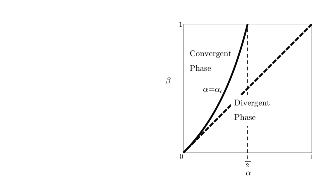
As we see Fig. 6, the region (42) is embedded in the region $\alpha<\beta$ where the usual M/M/1 queueing process converges. The critical line $\alpha=\alpha_{c}$ consists of two parts; a curve and a straight line. Mathematically, the curve is given by a solution to the denominator of the form (43) $=0$, and the straight line by a solution to $R=0$. Physically, the two parts correspond to the stationary current of the open TASEP in the high-density phase ($\beta<\min(1-\sqrt{1-p},\alpha)$) and the maximal-current phase ($\alpha,\beta\geq 1-\sqrt{1-p}$), respectively, see Table 1. This property is due to the form (35). In fact, the stationary current of the open TASEP on $L$-site chain with the entry probability 1 is given by

$$J_{L}=\frac{pc_{L}}{c_{L+1}+pc_{L}},$$ (44)

where $c_{L}$ is the coefficient of $\xi^{L}$ in ${\mathcal{Z}}(\xi,1)$. Note that the critical line for the continuous-time version of the model can be also written in terms of the stationary current of the continuous-time open TASEP [2], see Table 1 again.

Table 1: Comparison with the continuous-time model. In the second row, the settings of the models are given. In the third row, the stationary currents of the open TASEPs in the limit where the length of the chain $L\to\infty$ are described. In the fourth row, the critical lines of the exclusive queueing processes are described. The right column is obtained by taking the continuous-time limit of the left column.

discrete time (parallel update)	continuous time
entry probability $\alpha$	entry rate $\alpha$
exit probability $\beta$	exit rate $\beta$
hopping probability $p$	hopping rate $p$
$J_{\infty}$	$J_{\infty}$
$=\begin{cases}\displaystyle\frac{1-\sqrt{1-p}}{2}&\alpha,\beta\geq 1-\sqrt{1-p}\\ \displaystyle\frac{\alpha(p-\alpha)}{p-\alpha^{2}}&\alpha\leq\min(1-\sqrt{1-p},\beta)\\ \displaystyle\frac{\beta(p-\beta)}{p-\beta^{2}}&\beta<\min(1-\sqrt{1-p},\alpha)\end{cases}$	$=\begin{cases}\displaystyle\frac{p}{4}&\alpha,\beta\geq\frac{p}{2}\\ \displaystyle\alpha(1-\alpha/p)&\alpha\leq\min(\frac{p}{2},\beta)\\ \displaystyle\beta(1-\beta/p)&\beta<\min(\frac{p}{2},\alpha)\end{cases}$
$\alpha$	$\alpha$
$=\begin{cases}\displaystyle\frac{1-\sqrt{1-p}}{2}&\beta\geq 1-\sqrt{1-p}\\ \displaystyle\frac{\beta(p-\beta)}{p-\beta^{2}}&\beta<1-\sqrt{1-p}\end{cases}$	$=\begin{cases}\displaystyle\frac{p}{4}&\beta\geq\frac{p}{2}\\ \displaystyle\beta(1-\beta/p)&\beta<\frac{p}{2}\end{cases}$

Let us calculate some average values in the stationary state. We can calculate the average length of the system (the position of the leftmost particle) and the average number of particles in the system by differentiating $\ln{\mathcal{Z}}(\xi,\zeta)$ with respect to $\xi$ and $\zeta$, respectively, as

$$\langle L\rangle= \xi\frac{\partial}{\partial\xi}\ln{\mathcal{Z}}(\xi,1)\bigg{|}_{\xi=\frac{\alpha}{p(1-\alpha)}}=\frac{\alpha p(R-p+2(1-\alpha))}{R(R-p+2(1-\alpha)\beta)},$$ (45)

$$\langle N\rangle= \frac{\partial}{\partial\zeta}\ln{\mathcal{Z}}\left(\frac{\alpha}{p(1-\alpha)},\zeta\right)\bigg{|}_{\zeta=1}=\frac{\alpha(1-\alpha)(p-2\alpha p+R)}{R(R-p+2(1-\alpha)\beta)}.$$ (46)

The number $N_{q}$ of particles in the queue (i.e., $N_{q}=\#\{j\geq 2|\tau_{j}=1\}$ for $\tau_{L}\tau_{L-1}\cdots\tau_{1}\in S$ and $N_{q}=0$ for $\emptyset$) is also one of the typical values in the queueing theory. We can calculate the average of $N_{q}$ as

$$\langle N_{q}\rangle= \frac{1}{Z}\frac{\partial}{\partial\zeta}\sum_{L\geq 2}\xi^{L}\langle W|\zeta D(\zeta D+E)^{L-2}(D+E)|V\,\rangle\bigg{|}_{\xi=\frac{\alpha}{p(1-\alpha)},\zeta=1}$$ (47)

$$= \frac{1}{Z}\frac{\partial}{\partial\zeta}\left[\left(1+\frac{p\xi(1-\zeta)}{\beta(1+p\xi\zeta)}\right){\mathcal{Z}}(\xi,\zeta)-\frac{\beta+p\xi}{\beta}\right]_{\xi=\frac{\alpha}{p(1-\alpha)},\zeta=1}$$ (48)

$$= \langle N\rangle-\frac{\alpha}{\beta}.$$ (49)

Derivation of the second equality is given in Appendix C.

Figure 6: Phase diagram for the parallel-update exclusive queueing process. The critical line $\alpha=\alpha_{c}$ (solid line) divides the parameter space into the convergent phase and the divergent phase. We drew the dashed line representing the critical line of the usual M/M/1 queueing process as well. Note that there is a region $\alpha_{c}<({\rm or}\leq)\alpha<\beta$ where the M/M/1 queueing process converges but our new model diverges.

5 Case $p=1$

In this section we treat the model with $p=1$, where the bulk hopping rule is nothing but one of the typical deterministic cellular automata, i.e., rule 184. This case was analyzed in [26]. The matrices and vectors have a two-dimensional representation

$$D=\left(\begin{array}[]{cc}\frac{1-\beta}{\beta}&0\\ \frac{1}{\sqrt{\beta}}&0\end{array}\right),\ E=\left(\begin{array}[]{cc}0&\frac{1}{\sqrt{\beta}}\\ 0&0\end{array}\right),\ \langle W|=\left(1,\sqrt{\beta}\right),\ |V\rangle=\left(\begin{array}[]{c}1\\ \sqrt{\beta}\end{array}\right),$$ (56)

see [22].

In the case where $p=1$, each particle necessarily hops if its right neighbor site is empty. Thus, any configurations containing at least one sequence 00 vanish in the stationary state. In fact, we can see

$$P(1\tau_{L-1}\dots 00\dots\tau_{1})=\frac{1}{Z}\left(\frac{\alpha}{1-\alpha}\right)^{L}\langle W|\cdots EE\cdots|V\,\rangle=0.$$ (57)

One can reduce the stationary-state probability to the following simpler expression: for $\tau=\tau_{L}\tau_{L-1}\cdots\tau_{1}$ ($\tau_{L}=1$),

$$P(\tau)=\begin{cases}0&{\rm if}\ \tau\ {\rm contains\ a\ sequence\ 00}\\ \frac{1}{Z}\left(\frac{\alpha}{1-\alpha}\right)^{L}\frac{(1-\beta)^{2\#\{j|\tau_{j}=1\}-L-\tau_{1}}}{\beta^{\#\{j|\tau_{j}=1\}}}&{\rm otherwise}\end{cases}$$ (58)

Thanks to the two dimensional representation, calculating ${\mathcal{Z}}(\xi,\zeta)$ is an easy exercise:

$${\mathcal{Z}}(\xi,\zeta)= 1+\xi\zeta\langle W|D(1-\xi(\zeta D+E))^{-1}|V\rangle=\frac{1}{1-\frac{\xi\zeta(1+\xi)}{\beta(1+\xi\zeta)}},$$ (59)

$$Z= \frac{\beta(1-\alpha)}{\beta-\alpha-\alpha\beta}.$$ (60)

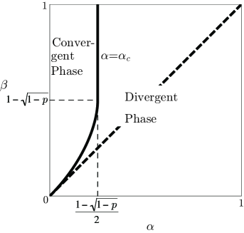
The square root vanishes from $Z$, and thus the critical line loses the straight line part, see Fig. 7:

$$\alpha_{c}=\frac{\beta}{1+\beta}.$$ (61)

The average length and the average numbers of particles in the system and the queue are simplified as

$$\langle L\rangle=\frac{\alpha}{\beta-\alpha-\alpha\beta},\quad\langle N\rangle=\frac{\alpha(1-\alpha)}{\beta-\alpha-\alpha\beta},\quad\langle N_{q}\rangle=\frac{\alpha^{2}}{\beta(\beta-\alpha-\alpha\beta)}.$$ (62)

It is also easy to calculate the probability distributions of $L$ and $N$ by expanding ${\mathcal{Z}}(\xi,1)$ and ${\mathcal{Z}}(\frac{\alpha}{1-\alpha},\zeta)$ around $\xi=0$ and $\zeta=0$, respectively:

$$\begin{split}&{\rm Prob}[\text{the length of the system}=L]\\ &=\frac{1}{Z}\left(\frac{\alpha}{1-\alpha}\right)^{L}\frac{1}{L!}\left.\frac{\partial^{L}{\mathcal{Z}}(\xi,1)}{\partial\xi^{L}}\right|_{\xi=0}=\frac{\beta-\alpha\beta-\alpha}{\beta(1-\alpha)}\left(\frac{\alpha}{\beta(1-\alpha)}\right)^{L},\end{split}$$ (63)

$$\begin{split}&{\rm Prob}[\text{the number of particles in the system}=N]\\ &=\frac{1}{Z}\frac{1}{N!}\left.\frac{\partial^{N}{\mathcal{Z}}(\frac{\alpha}{1-\alpha},\zeta)}{\partial\zeta^{N}}\right|_{\zeta=0}\\ &=\begin{cases}\displaystyle\frac{\beta-\alpha\beta-\alpha}{\beta(1-\alpha)}&N=0,\\ \displaystyle\frac{\beta-\alpha\beta-\alpha}{\beta(1-\beta+\alpha\beta)(1-\alpha)}\left(\frac{\alpha(1-\beta+\alpha\beta)}{\beta(1-\alpha)^{2}}\right)^{N}&N\geq 1.\end{cases}\end{split}$$ (64)

Figure 7: Phase diagram for $p=1$. The critical line $\alpha=\alpha_{c}$ (solid line) divides the parameter space into the convergent phase and the divergent phase. We drew the dashed line representing the critical line of the usual M/M/1 queueing process as well. Note that there is a region $\alpha_{c}\leq\alpha<\beta$ where the M/M/1 queueing process converges but our new model diverges.

6 Conclusion

In this paper, we introduced an extension of the discrete-time M/M/1 queueing process with excluded-volume effect (exclusive queueing process). We took the parallel-update scheme. A stationary-state solution was obtained in a slightly arranged matrix product form for the parallel-update open TASEP. We found that the critical line which separates the parameter space into regions with and without the stationary state is given by the stationary current of the open TASEP in the maximal-current and high-density phases. Particularly, we should note that the entry rate cannot be greater than the maximal current of the TASEP if the model converges. We calculated the average length of the system (the position of the leftmost particle) and the average number of particles in the system. These results recover the stationary state, the critical line and the average values of the continuous-time version of the exclusive queueing process [2], in the limit where the time interval $\Delta t\to 0$. In this sense, our discrete-time model is a generalization of the continuous-time model. We calculated the number of particles in the queue as well.

When $p=1$, i.e. the bulk hopping is deterministic, the matrices and the vectors constructing the stationary-state solution have a two-dimensional representation. The probability distributions of the length of the system and the average number of particles are both geometric in this case.

We leave calculations of the density profile and correlation functions in the stationary state as future works. In the TASEP with the ordinary open boundary condition, a domain wall theory explains its phase diagram successfully [18]. Investigating how our model converges to the stationary state or diverges with a similar argument will be also an interesting study.

Appendix A Reduction of the balance equation

In this section, we derive Eqs. (23)-(25). We calculate the action of ${\mathcal{T}}$ on $P$ under the assumption (13) and (14). Let us use a short hand notation $a=\frac{\alpha}{p(1-\alpha)}$. For a configuration $11\tau$ with $|11\tau|=L$, the action of ${\mathcal{T}}$ is calculated as

$$\begin{split}&Z{\mathcal{T}}P(11\tau)\\ =&Z\sum_{\tau^{\prime}\in{\mathcal{A}}_{11}(\tau)}W(11\tau^{\prime}\to 11\tau)P(11\tau^{\prime})+Z\sum_{\tau^{\prime}\in{\mathcal{A}}_{11}(\tau)}W(101\tau^{\prime}\to 11\tau)P(101\tau^{\prime})\\ &+Z\sum_{\tau^{\prime}\in{\mathcal{A}}_{11}(\tau)}W(1\tau^{\prime}\to 11\tau)P(1\tau^{\prime})\\ =&\sum_{\tau^{\prime}\in{\mathcal{A}}_{11}(\tau)}W(11\tau^{\prime}\to 11\tau)a^{L}f_{L}(11\tau^{\prime})+\sum_{\tau^{\prime}\in{\mathcal{A}}_{11}(\tau)}W(101\tau^{\prime}\to 11\tau)a^{L+1}f_{L+1}(101\tau^{\prime})\\ &+\sum_{\tau^{\prime}\in{\mathcal{A}}_{11}(\tau)}W(1\tau^{\prime}\to 11\tau)a^{L-1}f_{L-1}(1\tau^{\prime})\\ =&a^{L}\Bigg{(}\sum_{\tau^{\prime}\in{\mathcal{A}}_{11}(\tau)}\frac{1}{1-\alpha}W(11\tau^{\prime}\to 11\tau)f_{L}(11\tau^{\prime})\\ &\quad\quad\quad\quad\quad\quad\quad\quad\quad+\sum_{\tau^{\prime}\in{\mathcal{A}}_{11}(\tau)}\frac{1}{\alpha}W(1\tau^{\prime}\to 11\tau)f_{L}(01\tau^{\prime})\Bigg{)},\end{split}$$ (65)

where we used

$$W(101\tau^{\prime}\to 11\tau)=pW(11\tau^{\prime}\to 11\tau)=\frac{p(1-\alpha)}{\alpha}W(1\tau^{\prime}\to 11\tau)$$ (66)

and

$$f_{L+1}(101\tau^{\prime})=f_{L}(11\tau^{\prime})+pf_{L-1}(1\tau^{\prime}),\quad pf_{L-1}(1\tau^{\prime})=f_{L}(01\tau^{\prime}).$$ (67)

From $P(11\tau)={\mathcal{T}}P(11\tau)$, we get (23).

For a configuration $101\tau$ with $|101\tau|=L$, the action of ${\mathcal{T}}$ is calculated as

$$\begin{split}&Z{\mathcal{T}}P(101\tau)\\ =&Z\sum_{\tau^{\prime}\in{\mathcal{A}}_{101}(\tau)}W(101\tau^{\prime}\to 101\tau)P(101\tau^{\prime})+Z\sum_{\tau^{\prime}\in{\mathcal{A}}_{101}(\tau)}W(110\tau^{\prime}\to 101\tau)P(110\tau^{\prime})\\ &+Z\sum_{\tau^{\prime}\in{\mathcal{A}}_{101}(\tau)}W(10\tau^{\prime}\to 101\tau)P(10\tau^{\prime})+Z\sum_{\tau^{\prime}\in{\mathcal{A}}_{101}(\tau)}W(1010\tau^{\prime}\to 101\tau)P(1010\tau^{\prime})\\ &+Z\sum_{\tau^{\prime}\in{\mathcal{A}}_{101}(\tau)}W(1001\tau^{\prime}\to 101\tau)P(1001\tau^{\prime})\\ =&\sum_{\tau^{\prime}\in{\mathcal{A}}_{101}(\tau)}W(101\tau^{\prime}\to 101\tau)a^{L}f_{L}(101\tau^{\prime})+\sum_{\tau^{\prime}\in{\mathcal{A}}_{101}(\tau)}W(110\tau^{\prime}\to 101\tau)a^{L}f_{L}(110\tau^{\prime})\\ &+\sum_{\tau^{\prime}\in{\mathcal{A}}_{101}(\tau)}W(10\tau^{\prime}\to 101\tau)a^{L-1}f_{L-1}(10\tau^{\prime})+\sum_{\tau^{\prime}\in{\mathcal{A}}_{101}(\tau)}W(1010\tau^{\prime}\to 101\tau)a^{L+1}f_{L+1}(1010\tau^{\prime})\\ &+\sum_{\tau^{\prime}\in{\mathcal{A}}_{101}(\tau)}W(1001\tau^{\prime}\to 101\tau)a^{L+1}f_{L+1}(1001\tau^{\prime})\\ =&a^{L}\Bigg{(}\sum_{\tau^{\prime}\in{\mathcal{A}}_{101}(\tau)}\frac{1}{1-\alpha}W(101\tau^{\prime}\to 101\tau)f_{L}(101\tau^{\prime})+\sum_{\tau^{\prime}\in{\mathcal{A}}_{101}(\tau)}\frac{1}{1-\alpha}W(110\tau^{\prime}\to 101\tau)f_{L}(110\tau^{\prime})\\ &+\sum_{\tau^{\prime}\in{\mathcal{A}}_{101}(\tau)}\frac{1}{\alpha}W(10\tau^{\prime}\to 101\tau)f_{L}(010\tau^{\prime})\Bigg{)},\end{split}$$ (68)

where we used

$$W(1001\tau^{\prime}\to 101\tau)= \frac{p}{1-p}W(101\tau^{\prime}\to 101\tau),$$ (69)

$$W(1010\tau^{\prime}\to 101\tau)= pW(110\tau^{\prime}\to 101\tau)=\frac{p(1-\alpha)}{\alpha}W(10\tau^{\prime}\to 101\tau),$$ (70)

and

$$f_{L+1}(1010\tau^{\prime})=f_{L}(110\tau^{\prime})+pf_{L-1}(10\tau^{\prime}),$$ (71)

$$pf_{L-1}(10\tau^{\prime})=f_{L}(010\tau^{\prime}),\quad f_{L+1}(1001\tau^{\prime})=(1-p)f_{L}(101\tau^{\prime}).$$ (72)

From $P(101\tau)={\mathcal{T}}P(101\tau)$, we get (24).

For a configuration $100\tau$ with $|100\tau|=L$, the action of ${\mathcal{T}}$ is calculated as

$$\begin{split}&Z{\mathcal{T}}P(100\tau)\\ =&Z\sum_{\tau^{\prime}\in{\mathcal{A}}_{100}(\tau)}W(10\tau^{\prime}\to 100\tau)P(10\tau^{\prime})+Z\sum_{\tau^{\prime}\in{\mathcal{A}}_{100}(\tau)}W(100\tau^{\prime}\to 100\tau)P(100\tau^{\prime})\\ =&\sum_{\tau^{\prime}\in{\mathcal{A}}_{100}(\tau)}W(10\tau^{\prime}\to 100\tau)a^{L}f_{L}(10\tau^{\prime})+\sum_{\tau^{\prime}\in{\mathcal{A}}_{100}(\tau)}W(100\tau^{\prime}\to 100\tau)a^{L+1}f_{L+1}(100\tau^{\prime})\\ =&a^{L}\Bigg{(}\sum_{\tau^{\prime}\in{\mathcal{A}}_{100}(\tau)}\frac{1}{1-\alpha}W(10\tau^{\prime}\to 100\tau)f_{L}(10\tau^{\prime})\\ &+\sum_{\tau^{\prime}\in{\mathcal{A}}_{100}(\tau)}\frac{1}{(1-\alpha)(1-p)}W(10\tau^{\prime}\to 100\tau)f_{L}(00\tau^{\prime})\Bigg{)},\end{split}$$ (73)

where we used

$$W(100\tau^{\prime}\to 100\tau)=\frac{p}{1-p}W(10\tau^{\prime}\to 100\tau)$$ (74)

and

$$f_{L+1}(100\tau^{\prime})=(1-p)f_{L}(10\tau^{\prime}),\quad f_{L}(00\tau^{\prime})=0.$$ (75)

From $P(100\tau)={\mathcal{T}}P(100\tau)$, we get (25).

Appendix B Derivation of ${\mathcal{Z}}(\xi,\zeta)$

According to [11], $D,E,\langle W|$ and $|V\,\rangle$ can be reduced as

$$D=\left(\begin{array}[]{cc}D_{1}&0\\ D_{2}&0\end{array}\right),\quad E=\left(\begin{array}[]{cc}E_{1}&E_{2}\\ 0&0\end{array}\right),\quad\langle W|=(\ \langle W_{1}|\quad\langle W_{2}|\ ),\quad|V\,\rangle=\left(\begin{array}[]{c}|V_{1}\,\rangle\\ |V_{2}\,\rangle\end{array}\right),$$ (82)

where matrices $D_{1},D_{2},E_{1}$ and $E_{2}$, and vectors $\langle W_{1}|,\langle W_{2}|,|V_{1}\,\rangle$ and $|V_{2}\,\rangle$ satisfy

$$D_{1}E_{1}=(1-p)(D_{1}+E_{1}+p),$$ (83)

$$D_{1}|V_{1}\,\rangle=\frac{p(1-\beta)}{\beta}|V_{1}\,\rangle,\quad\langle W_{1}|E_{1}=0,$$ (84)

$$E_{2}D_{2}=p(D_{1}+E_{1}+p),$$ (85)

$$E_{2}|V_{2}\,\rangle=p|V_{1}\,\rangle,\quad\langle W_{2}|D_{2}=\langle W_{1}|p.$$ (86)

We can easily show that $D,E,\langle W|$ and $|V\,\rangle$ satisfy the relations (33) from the relation (83)-(86). In view of the normalization (34), we impose $\langle W_{1}|V_{1}\rangle=1$. The following gives a representation for these matrices and vectors, which will not be used in calculating ${\mathcal{Z}}(\xi,\zeta)$:

$$\begin{split}\langle W_{1}|=(1,0,0,\dots),\quad\langle W_{2}|=\sqrt{\beta}(0,1,-\sqrt{1-p},(-\sqrt{1-p})^{2},\dots),\\ D_{1}=\left(\begin{array}[]{ccccc}\frac{p(1-\beta)}{\beta}&\sqrt{\frac{p(1-p)}{\beta}}&&&\\ &1-p&\sqrt{1-p}&&\\ &&1-p&\sqrt{1-p}&\\ &&&1-p&\ddots\\ &&&&\ddots\end{array}\right),\quad D_{2}=\sqrt{\frac{p}{1-p}}E_{1},\\ E_{1}=\left(\begin{array}[]{ccccc}0&&&&\\ \sqrt{\frac{p(1-p)}{\beta}}&1-p&&&\\ &\sqrt{1-p}&1-p&&\\ &&\sqrt{1-p}&1-p&\\ &&&\ddots&\ddots\end{array}\right),\quad E_{2}=\sqrt{\frac{p}{1-p}}D_{1},\\ |V_{1}\,\rangle=\left(\begin{array}[]{c}1\\ 0\\ 0\\ \vdots\end{array}\right),\quad|V_{2}\,\rangle=\frac{\beta}{1-\beta}\sqrt{\frac{1-p}{p}}|V_{1}\,\rangle,\end{split}$$ (87)

where we arranged the representation (6.6)-(6.11) in [11].

To calculate ${\mathcal{Z}}(\xi,\zeta)$, we imitate the calculation (59) for $p=1$ as

$$\begin{split}{\mathcal{Z}}(\xi,\zeta)=&1+\sum_{L\geq 1}\xi^{L}\langle W|\zeta D(\zeta D+E)^{L-1}|V\,\rangle\\ =&1+\xi\zeta\langle W|D(1-\xi(\zeta D+E))^{-1}|V\,\rangle\\ =&1+\xi\zeta\left(\ \langle W_{1}|\quad\langle W_{2}|\ \right)\left(\begin{array}[]{cc}D_{1}&0\\ D_{2}&0\end{array}\right){\left(\begin{array}[]{cc}1-\xi\zeta D_{1}-\xi E_{1}&\ -\xi E_{2}\\ -\xi\zeta D_{2}&1\end{array}\right)}^{-1}\left(\begin{array}[]{c}|V_{1}\,\rangle\\ |V_{2}\,\rangle\end{array}\right)\\ =&1+\xi\zeta\left(\ \langle W_{1}|\quad\langle W_{2}|\ \right)\left(\begin{array}[]{cc}D_{1}&0\\ D_{2}&0\end{array}\right){\left(\begin{array}[]{cc}X&\ \xi XE_{2}\\ \xi\zeta D_{2}X&\ 1+\xi^{2}\zeta D_{2}XE_{2}\end{array}\right)}\left(\begin{array}[]{c}|V_{1}\,\rangle\\ |V_{2}\,\rangle\end{array}\right)\\ =&1+\xi\zeta\left(\ \langle W_{1}|D_{1}+\langle W_{2}|D_{2}\ \right)\left(X|V_{1}\,\rangle+\xi XE_{2}|V_{2}\,\rangle\right),\end{split}$$ (88)

where $X^{-1}=1-\xi\zeta D_{1}-\xi E_{1}-\xi^{2}\zeta E_{2}D_{2}$. Using the relation (85), we can eliminate $D_{2}$ and $E_{2}$ in $X$ as

$$X^{-1}=(1-p^{2}\xi^{2}\zeta)-\xi\zeta(1+p\xi)D_{1}-\xi(1+p\xi\zeta)E_{1}.$$ (89)

Furthermore, using the relation (86), we can eliminate $D_{2},E_{2},\langle W_{2}|$ and $|V_{2}\,\rangle$ in ${\mathcal{Z}}(\xi,\zeta)$ as

$$\begin{split}{\mathcal{Z}}(\xi,\zeta)=&1+\xi\zeta\langle W_{1}|(D_{1}+p)X(1+p\xi)|V_{1}\,\rangle\\ =&1+\langle W_{1}|\left\{\xi\zeta(1+p\xi)D_{1}+p\xi\zeta(1+p\xi)\right\}X|V_{1}\,\rangle\\ =&1+\langle W_{1}|\left\{-X^{-1}+(1+p\xi\zeta)-\xi(1+p\xi\zeta)E_{1}\right\}X|V_{1}\,\rangle\\ =&(1+p\xi\zeta)\langle W_{1}|X|V_{1}\,\rangle.\end{split}$$ (90)

In the last equality, we used the second relation of (84) and $\langle W_{1}|V_{1}\rangle=1$. Now we borrow an idea from Section 4.3 of [4], where the generating function of the TASEP with a single defect particle on a ring was obtained. Set

$$D^{\prime}=aD_{1}+b,\quad E^{\prime}=cE_{1}+d$$ (91)

with $a=\sqrt{\frac{u}{1-p}},b=1-\sqrt{u(1-p)},c=\frac{1}{\sqrt{u(1-p)}}$ and $d=1-\sqrt{\frac{1-p}{u}}$, and we get

$$D^{\prime}E^{\prime} =D^{\prime}+E^{\prime}$$ (92)

$$\langle W_{1}|E^{\prime} =d\langle W_{1}|,\quad D^{\prime}|V_{1}\,\rangle=\left(\frac{p(1-\beta)}{\beta}a+b\right)|V_{1}\,\rangle=:f|V_{1}\,\rangle,$$ (93)

noting the relations (83) and (84). Set $u=\frac{\zeta(1+p\xi)}{1+p\xi\zeta}$, and we get

$$\begin{split}X^{-1}=&(1-p^{2}\xi^{2}\zeta)-\xi(1+p\xi\zeta)(E_{1}+uD_{1})\\ =&g-h(D^{\prime}+E^{\prime}),\end{split}$$ (94)

where

$$g=(1-p^{2}\xi^{2}\zeta)+\xi(1+p\xi\zeta)\frac{b+d}{c},\quad h=\frac{\xi(1+p\xi\zeta)}{c}.$$ (95)

Set $\omega(1-\omega)=\frac{h}{g}$, and we get

$$\begin{split}X=\frac{1}{g}\left(1-\frac{h}{g}(D^{\prime}+E^{\prime})\right)^{-1}=\frac{1}{g}\left(1-\omega E^{\prime}\right)^{-1}\left(1-\omega D^{\prime}\right)^{-1}.\end{split}$$ (96)

Finally, we achieve

$${\mathcal{Z}}(\xi,\zeta)=\frac{1+p\xi\zeta}{g}\langle W_{1}|\left(1-\omega E^{\prime}\right)^{-1}\left(1-\omega D^{\prime}\right)^{-1}|V_{1}\,\rangle=\frac{1+p\xi\zeta}{g(1-\omega d)(1-\omega f)},$$ (97)

which can be simplified as (38) and expanded as

$${\mathcal{Z}}(\xi,\zeta)= 1+\sum_{L\geq N\geq 1}a_{LN}\xi^{L}\zeta^{N},$$ (98)

$$\begin{split}a_{LN}=&(1-p)^{L-2N}\sum_{k=0}^{N}\frac{(L-k-1)!(N-1)!(-p)^{k}}{(L-N)!(N-k-1)!k!(N-k)!}\\ &\!\!\!\!\!\!\!\!\!\!\!\!\!\!\!\!\times\sum_{k=0}^{N-1}\left[\left(\frac{p}{\beta}\right)^{k+1}\frac{(L-k-2)!}{(N-k-1)!(L-N-1)!}\sum_{\ell=0}^{k}\frac{(k-\ell+1)\cdot N!}{\ell!(N-\ell)!}(-\beta)^{\ell}\right].\end{split}$$ (99)

Appendix C Derivation of $\langle N_{q}\rangle$

In this section, we show

$$\sum_{L\geq 2}\xi^{L}\langle W|\zeta D(\zeta D+E)^{L-2}(D+E)|V\,\rangle=\left(1+\frac{p\xi(1-\zeta)}{\beta(1+p\xi\zeta)}\right){\mathcal{Z}}(\xi,\zeta)-\frac{\beta+p\xi}{\beta}.$$ (100)

The left-hand side is calculated as

$$\begin{split}&\sum_{L\geq 2}\xi^{L}\langle W|\zeta D(\zeta D+E)^{L-2}(D+E)|V\,\rangle\\ =&\sum_{L\geq 1}\xi^{L}\langle W|D(\zeta D+E)^{L-1}|V\,\rangle\\ &-(1-\zeta)\sum_{L\geq 2}\xi^{L}\langle W|D(\zeta D+E)^{L-2}E|V\,\rangle-\xi\langle W|D|V\,\rangle\\ =&\frac{{\mathcal{Z}}(\xi,\zeta)-1}{\zeta}-\xi^{2}(1-\zeta)\langle W|D(1-\xi(\zeta D+E))^{-1}E|V\,\rangle-\frac{p\xi}{\beta}\end{split}$$ (101)

Recall the formula

$$(1-\xi(\zeta D+E))^{-1}=\left(\begin{array}[]{cc}X&\ \xi XE_{2}\\ \xi\zeta D_{2}X&\ 1+\xi^{2}\zeta D_{2}XE_{2}\end{array}\right).$$ (104)

Using this and the relations (84) and (86), we obtain

$$\begin{split}&\langle W|D(1-\xi(\zeta D+E))^{-1}E|V\,\rangle\\ &=\langle W_{1}|(D_{1}+p)X(E_{1}+p)|V_{1}\,\rangle\\ &=\langle W_{1}|\frac{(1+p\xi\zeta)-\xi(1+p\xi\zeta)E_{1}-X^{-1}}{\xi\zeta(1+p\xi)}X\frac{(1+p\xi)-\xi\zeta(1+p\xi)D_{1}-X^{-1}}{\xi(1+p\xi\zeta)}|V_{1}\,\rangle\\ &=\frac{\langle W_{1}|\left\{(1+p\xi\zeta)-X^{-1}\right\}X\left\{(1+p\xi)\left(1-\frac{p(1-\beta)\xi\zeta}{\beta}\right)-X^{-1}\right\}|V_{1}\,\rangle}{\xi^{2}\zeta(1+p\xi)(1+p\xi\zeta)}\end{split}$$ (105)

Finally, noting $\langle W_{1}|X|V_{1}\,\rangle=\frac{{\mathcal{Z}}(\xi,\zeta)}{1+p\xi\zeta}$, $\langle W_{1}|V_{1}\rangle=1$ and the relation (84), we achieve (100).

References

• [1]
• [2] Arita, C.: Queueing process with excluded-volume effect. Phys. Rev. E 80(5), 051119 (2009)
• [3] Barabasi, A.L.: The origin of bursts and heavy tails in human dynamics. Nature 435, 207–211 (2005)
• [4] Blythe, R.A., Evans, M.R.: Nonequilibrium steady states of matrix product form: A solver’s guide. J. Phys. A: Math. Gen. 40, R333 (2007)
• [5] Burke, P.J.: The output of a queuing system. Operations Research 4(6), 699–704 (1956)
• [6] Burstedde, C., Klauck, K., Schadschneider, A., Zittartz, J.: Simulation of pedestrian dynamics using a two-dimensional cellular automaton. Physica A 295, 507 (2001)
• [7] Chowdhury, D., Santen, L., Schadschneider, A.: Statistical physics of vehicular traffic and some related systems. Phys. Rep. 329, 199 (2000)
• [8] Derrida, B., Evans, M.R., Hakim, V., Pasquier, V.: An exact solution of a 1d asymmetric exclusion model using a matrix formulation. J. Phys. A: Math. Gen. 26, 1493 (1993)
• [9] Erlang, A.K.: The theory of probabilities and telephone conversations. Nyt. Tidsskr. Mat. Ser. B 20, 33–39 (1909)
• [10] Erlang, A.K.: Solution of some problems in the theory of probabilities of significance in automatic telephone exchanges. Post Office Electr. Eng. J. 10, 189–197 (1917)
• [11] Evans, M.R., Rajewsky, N., Speer, E.R.: Exact solution of a cellular automata for traffic. J. Stat. Phys. 95, 45–96 (1999)
• [12] Helbing, D., Jiang, R., Treiber, M.: Analytical investigation of oscillations in intersecting flows of pedestrian and vehicle traffic. Phys. Rev. E 72, 046130 (2005)
• [13] Helbing, D., Treiber, M., Kesting, A.: Understanding interarrival and interdeparture time statistics from interactions in queueing systems. Physica A 363, 62–72 (2006)
• [14] Jackson, J.R.: Networks of waiting lines. Operations Research 5(4), 518–521 (1957)
• [15] Jain, J.L., Mohanty, S.G., Böhm, W.: A Course on Queueing Models, Chapman & Hall/CRC, Boca Raton (2006)
• [16] Kendall, D.G.: Some problems in the theory of queues. J. Roy. Statist. Soc. Ser. B 13(2), 151–158 (1951)
• [17] Kendall, D.G.: Stochastic processes occurring in the theory of queues and their analysis by the method of the imbedded Markov chain. Ann. Math. Statist. 24(3), 338–354 (1953)
• [18] Kolomeisky, A.B., Schütz, G.M., Kolomeisky, E.B., Straley, J.P.: Phase diagram of one-dimensional driven lattice gases with open boundaries. J. Phys. A: Math. Gen. 31 6911 (1998)
• [19] Liggett, T. M.: Stochastic Interacting Systems: Contact, Voter and Exclusion Processes, Springer, New York (1999)
• [20] Little, J.C.D.: A proof for the queuing formula: L=λW𝐿𝜆𝑊L=\lambda W. Operations Research 9(3), 383–387 (1961)
• [21] Mukherjee, G., Manna, S.S.: Phase transition in a directed traffic flow network. Phys. Rev. E 71, 066,108 (2005)
• [22] Rajewsky, N., Santen, L., Schadschneider, A., Schreckenberg, M.: The asymmetric exclusion process: Comparison of update procedures. J. Stat. Phys. 92, 151 (1998)
• [23] Rogsch, C., Schadschneider, A., Seyfried, A., Klingsch, W.: How to select the “right one” - update schemes for pedestrian movement in simulation and reality. Proceedings of the Traffic and Granular Flow ’09 (to be published)
• [24] Schinazi, R. B.: Classical and spatial stochastic processes, Birkhäuser, Boston (1999)
• [25] Schütz, G.M.: Exactly solvable models for many-body systems far from equilibrium, Phase transitions and critical phenomena, Vol. 19, C. Domb and J. Lebowitz eds., Academic, New York (2001)
• [26] Yanagisawa, D., Tomoeda, A., Jiang, R., Nishinari, K.: Excluded volume effect in queueing theory. JSIAM Lett. 2, 61 (2010)